Causal Diffusion and the Survival of Charge Fluctuations in Nuclear Collisions

Abstract

Diffusion may obliterate fluctuation signals of the QCD phase transition in nuclear collisions at SPS and RHIC energies. We propose a hyperbolic diffusion equation to study the dissipation of net charge fluctuations. This equation is needed in a relativistic context, because the classic parabolic diffusion equation violates causality. We find that causality substantially limits the extent to which diffusion can dissipate these fluctuations.

I Introduction

Net-charge fluctuations are measured in nuclear collisions by many RHIC and SPS experiments Mitchell . Conserved quantities such as net electric charge, baryon number, and strangeness can fluctuate when measured in limited rapidity intervals. These fluctuations occur mainly because the number of produced particles varies with each collision event due to differences in impact parameter, energy deposition, and baryon stopping. A variety of interesting dynamic effects can also contribute to these fluctuations EarlyFluctuations . In particular, fluctuations of mean $p_{t}$, net charge, and baryon number may probe the hadronization mechanism of the quark-gluon plasma RajagopalShuryakStephanov .

Fluctuations of conserved quantities are perhaps the best probes of hadronization, because conservation laws limit the dissipation they suffer after hadronization has occurred JeonKoch ; BowerGavin . This dissipation occurs by diffusion. While the effect of diffusion on charge and baryon fluctuations has been studied in refs. ShuryakStephanov ; BowerGavin , the classic diffusion equations used are problematic in a relativistic context, because they allow signals to propagate with infinite speed, violating causality.

In this paper we study the dissipation of net charge fluctuations in RHIC collisions using a causal diffusion equation. We find that causality inhibits dissipation, so that extraordinary fluctuations, if present, may survive to be detected. In sec. II we discuss how the classic approach to diffusion violates causality, and present a causal equation that resolves this problem. The derivation we include facilitates our work in later sections. We generalize this equation for relativistic fluids in nuclear collisions in sec. III. Related causal fluid equations for viscosity and heat conduction have been introduced in muronga and teaney with different heavy-ion applications in mind.

Our causal formulation can be crucial for the description of net-charge fluctuations, which involve rapid changes in the inhomogeneous collision environment aziz . We turn to this problem in secs. IV–VI. In sec. IV we discuss fluctuation measurements and their relation to two-particle correlation functions. In sec. V we introduce techniques from VanKampen to compute the effect of causal and classic diffusion on these correlation functions. We then estimate the impact of causal diffusion on fluctuation measurements in sec. VI. These three sections are close in spirit to work by Shuryak and Stephanov, where a classic diffusion model is used ShuryakStephanov .

II causal diffusion

To understand why the propagation speed in classic diffusion is essentially infinite, recall that the diffusion of particles through a medium is equivalent to a random walk in the continuum limit. The variance of the particle’s displacement increases by $d^{2}\equiv\langle\Delta x^{2}\rangle\propto\Delta t$ in the time interval $\Delta t$ between random steps. The average propagation speed $v\sim d/\Delta t$ diverges in the continuum limit, where $\Delta t\rightarrow 0$ with the diffusion coefficient $D=d^{2}/\Delta t$ held fixed. Correspondingly, a delta function density spike is instantaneously spread by diffusion into a Gaussian, with tails that extend to infinity.

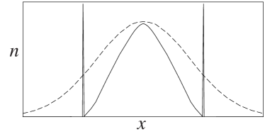
Figure 1: Density vs. position for causal (solid) and classic (dashed) diffusion assuming an initial delta function distribution. The spikes represent the right and left moving diffusion fronts of velocity $v=\pm(D/\tau_{d})^{1/2}$.

A causal alternative to the diffusion equation is the Telegraph equation,

$$\tau_{d}{{\partial^{2}}\over{\partial t^{2}}}n+{{\partial}\over{\partial t}}n=D\nabla^{2}n,$$ (1)

where $D$ is the diffusion coefficient and $\tau_{d}$ is the relaxation time for diffusion telegraph ; grad ; israel . Signals propagate at the finite speed $v=(D/\tau_{d})^{1/2}$, so that a delta function spike spreads behind a front travelling at $v$, as shown in fig. 1. The classic diffusion equation omits the term $\propto\tau_{d}$. Classic diffusion describes the matter well behind the front at times $t\gg\tau_{d}$. This contrasting behavior is generic of hyperbolic equations such as (1), which include a second order time derivative, compared to parabolic equations, like the classic first-order diffusion equation zauderer .

Causality concerns are not restricted to relativistic quarks or pions diffusing through a quark gluon plasma or hadron gas. They are common – and constantly debated – whenever time varying diffusion and heat conduction phenomena are discussed Mandelis . However, for most nonrelativistic systems, causality violations are minuscule, so that classic diffusion can be used. This need not be the case for relativistic fluids produced in nuclear collisions muronga ; aziz ; teaney .

To motivate (1) and understand its limitations, we first derive the diffusion coefficient using the Boltzmann equation in the relaxation time approximation; see, e.g., Gavin85 . Equation (1) can also be obtained by the moment method muronga or by sum-rule arguments forster . For simplicity, we focus on electric charge transport by a single species. Generalization to multiple species and other currents such as baryon number is straightforward, except for the challenging case of color transport Mrowczynski . We describe the evolution of the phase space distribution $f$ using

$${{\partial f}\over{\partial t}}+\mathbf{v}_{\mathbf{p}}\cdot\nabla f=-\nu(f-f_{e}),$$ (2)

where $\nu^{-1}$ is the relaxation time, $\mathbf{v}_{\mathbf{p}}=\mathbf{p}/E$, and $E=\{p^{2}+m^{2}\}^{1/2}$. The local equilibrium distribution satisfies $f_{e}=\{\exp[(E-\mu)/T]\pm 1\}^{-1}$ where $T$ is the temperature $T$, $\mu$ the chemical potential, and the $+$ or $-$ sign describes bosons or fermions.

Suppose that $\mu$ differs from a local equilibrium value by a small sinusoidally varying perturbation $\delta\mu$, with $\delta n=(\partial n/\partial\mu)\delta\mu$. Then $f$ is driven from local equilibrium by an amount $\delta f(\omega,\mathbf{k})\exp\{i\mathbf{k}\cdot\mathbf{x}-i\omega t\}$. Equation (2) implies

$$\delta f(\omega,\mathbf{k})=-{i{\mathbf{v}_{\mathbf{p}}\cdot\mathbf{k}}\over{\nu-i(\omega-\mathbf{k}\cdot\mathbf{v}_{\mathbf{p}})}}{{\partial f_{e}}\over{\partial\mu}}\delta\mu(\omega,\mathbf{k}),$$ (3)

plus corrections of order $\nu^{-2}$. The net charge current is

$$\delta\mathbf{j}(\omega,\mathbf{k})\equiv\int\delta f(\omega,\mathbf{k})\mathbf{v}_{\mathbf{p}}d\mathbf{p}=-i\mathbf{k}D(\omega,\mathbf{k})\delta n(\omega,\mathbf{k}),$$ (4)

where $d\mathbf{p}=d^{3}p/(2\pi)^{3}$. The diffusion coefficient is

$$D(\omega,\mathbf{k})={{1}\over{3}}{{\partial\mu}\over{\partial n}}\int{{v_{\mathbf{p}}^{2}}\over{\nu-i(\omega-\mathbf{k}\cdot\mathbf{v}_{\mathbf{p}})}}{{\partial f_{e}}\over{\partial\mu}}d\mathbf{p},$$ (5)

which is a relativistic generalization of a completely standard kinetic theory result. For $\mathbf{k}=\omega=0$, we recover the familiar static diffusion coefficient $D=\nu^{-1}v_{\rm th}^{2}/3$, where the thermal velocity $v_{\rm th}=1$ for massless particles. To obtain quantitative results from this relaxation time approximation, we identify $\nu^{-1}$ with the relaxation time for diffusion $\tau_{d}$ obtained by more sophisticated methods, see e.g. Prakash ; PVW ; HeiselbergPethick ; Moore ; diffusion .

To obtain (1), we omit the $\mathbf{k}$ dependence in (5), to find

$$D(\omega,0)=D/(1-i\omega\tau_{d}),$$ (6)

where $D$ is the static diffusion coefficient and $\nu^{-1}=\tau_{d}$. We then write

$$(1-i\omega\tau_{d})\mathbf{j}(\omega,\mathbf{k})=-i\mathbf{k}Dn(\omega,\mathbf{k}),$$ (7)

to find

$$\tau_{d}\frac{\partial}{\partial t}\mathbf{j}(\mathbf{x},t)+\mathbf{j}(\mathbf{x},t)=-D\mathbf{\nabla}n(\mathbf{x},t),$$ (8)

the Maxwell-Cattaneo relation telegraph . Combining (8) with current conservation $\partial n/\partial t+\mathbf{\nabla}\cdot\mathbf{j}=0$ yields (1). We will extend this argument in sec. V to derive eq. (40).

Classic diffusion follows from (8) when the $\tau_{d}$ term is negligible, a result known as Fick’s law. Fick’s law violates causality because any density change instantaneously causes current to flow. Including the $\tau_{d}$ term is the simplest way to incorporate a causal time lag for this current response forster . Moreover, (8) is self consistent in that it saturates the $f$-sum rule forster . However, while (1) is a plausible approximation, the $k\rightarrow 0$ limit (7) is not strictly justified. Possible generalizations can include the nonlocal equations or gradient expansions derived from (3) and (5). If (1) leads to substantial corrections to classic diffusion, then such generalizations can be worth considering.

In solving (1) we must impose initial conditions on the current that respect causality. Suppose that we introduce a density pulse at $\mathbf{x}=0$ at time $t=0$. Microscopically, particles begin to stream freely away from this point. The current implied by (8) is

$$\mathbf{j}(t)=\mathbf{j}(0)e^{-t/\tau_{d}}-\int_{0}^{t}{{ds}\over{\tau_{d}}}e^{-(t-s)/\tau_{d}}D\mathbf{\nabla}n(s).$$ (9)

Scattering with the surrounding medium eventually establishes a steady state in which Fick’s law holds, as we see from (8) for $\partial\mathbf{j}/\partial t=0$, but this takes a time $t\gg\tau_{d}$. An assumption of no initial flow $\mathbf{j}(0)=0$ is consistent with our physical picture, since there is no preferred direction for the initial velocity of each particle. Note that an alternative choice $\mathbf{j}(0)=-D\mathbf{\nabla}n(0)$ would imply that the current always follows Fick’s law; the corresponding solutions of (1) would never differ appreciably from classic diffusion. However, this choice is not causal because it requires that particles “know” about the medium before they have had any opportunity to interact with it.

III ion collisions

We now extend (1) to study the diffusion of charge through the relativistic fluid produced in a nuclear collision. The fluid flows with four velocity $u^{\mu}$ determined by solving the hydrodynamic equations $\partial_{\mu}T^{\mu\nu}=0$ together with the appropriate equation of state. We choose the Landau-Lifshitz definition of $u^{\mu}$ in terms of momentum current degroot . For sufficiently high energy collisions, the relative concentration of net charge is small enough that it has no appreciable impact on $u^{\mu}$. Correspondingly, we take $u^{\mu}$ to be a fixed function of $\mathbf{x}$ and $t$.

Following degroot , we define the co-moving time derivative and gradient

$$D_{\tau}\equiv u^{\mu}\partial_{\mu}\,\,\,\,{\rm and}\,\,\,\,\nabla^{\mu}=\partial^{\mu}-u^{\mu}u^{\nu}\partial_{\nu}$$ (10)

for the metric $g^{\mu\nu}={\rm diag}(1,-1,-1,-1)$. In the local rest frame where $u^{\mu}=(1,0,0,0)$, these quantities are the time derivative and $-\mathbf{\nabla}$, where $\mathbf{\nabla}$ is the three-gradient. The total charge current in the moving fluid is $j_{\rm tot}^{\mu}=nu^{\mu}+j^{\mu}$, where the first contribution is due to flow and the second to diffusion. Continuity then implies

$$\partial_{\mu}(nu^{\mu})=-\partial_{\mu}j^{\mu}.$$ (11)

We assume that the diffusion current satisfies

$$\tau_{d}D_{\tau}j^{\mu}+j^{\mu}=D\nabla^{\mu}n,$$ (12)

which reduces to (8) in the local rest frame.

To illustrate the effect of flow on diffusion, we consider longitudinal Bjorken flow, $u^{\mu}=(t/\tau,0,0,z/\tau)$, where $\tau=(t^{2}-z^{2})^{1/2}$, $\eta=(1/2)\log((t+z)/(t-z))$, the density is a function only of $\tau$ and the current is $j^{\mu}=(j^{t},0,0,j^{z})$ Bjorken . The continuity equation (11) is then

$$\left(\frac{\partial}{\partial\tau}+\frac{1}{\tau}\right)n=\frac{1}{\tau}\frac{\partial}{\partial\tau}(\tau n)=-\partial_{\mu}j^{\mu}.$$ (13)

To evaluate the covariant Maxwell-Cattaneo relation, we differentiate (12) to find

$$\tau_{d}\partial_{\mu}(u^{\nu}\partial_{\nu}j^{\mu})+\partial_{\mu}j^{\mu}=-D\nabla^{2}n,$$ (14)

where $\nabla^{2}\equiv\nabla_{\mu}\nabla^{\mu}$. We then write

$$\partial_{\mu}(u^{\nu}\partial_{\nu}j^{\mu}) = (\partial_{\mu}u^{\nu})(\partial_{\nu}j^{\mu})+u^{\nu}\partial_{\nu}(\partial_{\mu}j^{\mu})$$ (15)

$$= \frac{1}{\tau}\partial_{\mu}j^{\mu}+\frac{\partial}{\partial\tau}(\partial_{\mu}j^{\mu}),$$

where the second line follows from eqs. (17) and (20) of ref. Bjorken . Then (14) and (15) imply

$$\tau_{d}\frac{\partial}{\partial\tau}(\tau\partial_{\mu}j^{\mu})+\tau\partial_{\mu}j^{\mu}=-D\nabla^{2}n\tau.$$ (16)

Together, (13) and (16) describe causal diffusion.

To obtain an equation analogous to (1) for the expanding system, observe that the rapidity density $\rho\equiv dN/d\eta=A_{\bot}n\tau$, where $A_{\bot}$ is the transverse area of the two colliding nuclei. If one identifies spatial rapidity $\eta$ with the momentum-space rapidity of particles, then $\rho$ is observable. We combine (13) and (16) to find that this rapidity density satisfies

$$\tau_{d}\frac{\partial^{2}\rho}{\partial\tau^{2}}+\frac{\partial\rho}{\partial\tau}=\frac{D}{\tau^{2}}\frac{\partial^{2}\rho}{\partial\eta^{2}},$$ (17)

where $\nabla^{2}=\tau^{-2}\partial^{2}/\partial\eta^{2}$ for longitudinal expansion. Initial conditions for $\rho$ and $\partial\rho/\partial\tau$ at the formation time $\tau_{o}$ must be specified. In view of the causality argument surrounding (9), we assume that the initial diffusion current $j^{\mu}\equiv 0$, so that (13) implies $\partial\rho/\partial\tau\equiv 0$ at $\tau=\tau_{o}$. Note that the total current $nu^{\mu}+j^{\mu}$ is initially non-zero, since the underlying medium is not at rest.

In the absence of diffusion, longitudinal expansion leaves $\rho$ fixed, as we see from (13) for $j\equiv 0$. Diffusion tends to broaden the rapidity distribution. To characterize this broadening, we compute the rapidity width defined by $V\equiv\langle(\eta-\langle\eta\rangle)^{2}\rangle=N^{-1}\int\eta^{2}\rho d\eta$, where $\langle\eta\rangle=0$ and $N=\int\rho d\eta$. We multiply both sides of (17) by $\eta^{2}$ and integrate to find

$$\tau_{d}\frac{\partial^{2}{V}}{\partial\tau^{2}}+\frac{\partial{V}}{\partial\tau}=\frac{2D}{\tau^{2}}.$$ (18)

Observe that classic diffusion follows from (18) for $\tau_{d}=0$ with $D$ fixed. In that case the width increases by

$$\Delta V=\frac{2D}{\tau_{o}}\left(1-\frac{\tau_{o}}{\tau}\right),\quad\quad\quad\quad{\rm classic}$$ (19)

where $\Delta V\equiv{V}-{V}(\tau_{o})$. The rapidity width indeed increases, but the competition between longitudinal expansion and diffusion limits this increase to an asymptotic value $V_{\infty}=2D/\tau_{o}$.

We now solve (18) for causal diffusion to obtain

$$\Delta V=\frac{2D}{\tau_{o}}\int_{1}^{\tau/\tau_{o}}F(\alpha,\lambda)d\lambda,$$ (20)

where $\alpha\equiv\tau_{o}/\tau_{d}$ and

$$F(\alpha,\lambda)=\alpha\int_{1}^{\lambda}\xi^{-2}e^{\alpha(\xi-\lambda)}d\xi.$$ (21)

We have taken $dV/d\tau=0$ at $\tau=\tau_{o}$, as required when the initial $\partial\rho/\partial\tau$ vanishes. Figure 2 compares $\Delta V/V_{\infty}$ for classic and causal diffusion. We find that the rapidity broadening is always slower for causal diffusion compared to the classic case. These solutions approach one another for $\tau\gg\tau_{o}$; they are within 20% for $\tau>1.4~{}\tau_{o}$ for $\alpha=10$. The classic result (19) follows from (20) and (21) for $\alpha=\tau_{o}/\tau_{d}\rightarrow\infty$.

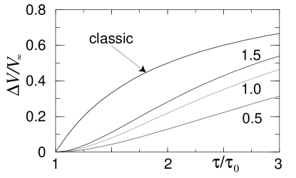
Figure 2: Rapidity spread vs. time for causal and classic diffusion computed using (20) and (19) respectively. Causal curves are for $\tau_{o}/\tau_{d}=0.5$, 1, and 1.5. Rapidity spreads are divided by the asymptotic value $V_{\infty}=2D/\tau_{o}$.

We have so far assumed that $\tau_{d}$ and $D$ are constant, but this may not be the case. These coefficients can vary with the overall density as the system expands and rarefies. As an alternative extreme, suppose that diffusion occurs as massless charged particles elastically scatter with the expanding fluid of density $n_{\rm tot}$. Kinetic theory implies that $\tau_{d}^{-1}\approx\langle\sigma v_{\rm rel}\rangle n_{\rm tot}$ and $D\approx\tau_{d}/3$. If we take the scattering rate $\langle\sigma v_{\rm rel}\rangle$ averaged over species and temperature to be constant, but assume $n_{\rm tot}\propto\tau^{-1}$ as determined by entropy conservation, then $\tau_{d}\propto D\propto\tau$. Realistically, particle-mass effects would reduce the rate of growth of $\tau_{d}$ and $D$, as would the temperature dependence of $\langle\sigma v_{\rm rel}\rangle$. Nevertheless, the linear growth rate is worth considering to illustrate how rarefaction can change the results.

Including this extreme effect of rarefaction implies $\tau_{d}=\tau_{d}(\tau_{o})\tau/\tau_{o}$, so that

$$\tau_{d}=\tau/\alpha,$$ (22)

where we now fix the parameter $\alpha=\tau_{o}/\tau_{d}(\tau_{o})$ at the initial time. Taking $D=\tau_{d}/3$ gives

$$D=\tau/3\alpha,$$ (23)

so that the diffusion equation (18) becomes

$$\tau\frac{d^{2}{V}}{d\tau^{2}}+\alpha\frac{d{V}}{d\tau}=\frac{2}{3\tau}.$$ (24)

As before, classic diffusion is obtained by omitting the second derivative term. We find

$$\Delta V=\frac{2}{3\alpha}\ln{{\tau}\over{\tau_{o}}}.\quad\quad\quad\quad{\rm classic}$$ (25)

We see that the width now increases without bound, which is not surprising since our time varying parameters (22, 23) imply that $V_{\infty}=2D/\tau_{o}\propto\tau$.

Informed by the classic case, we write the causal equation as

$$\frac{d^{2}{V}}{d\theta^{2}}+(\alpha-1)\frac{d{V}}{d\theta}=\frac{2}{3},$$ (26)

where $\theta=\ln{{\tau}/{\tau_{o}}}$. When $\alpha=1$, the first derivative vanishes, so that

$$\Delta V=(\ln\tau/\tau_{o})^{2}/3.$$ (27)

For $\alpha\neq 1$, we find

$$\Delta V=\frac{2}{3(\alpha-1)}\left\{\ln{{\tau}\over{\tau_{o}}}-\frac{1}{\alpha-1}\left[1-{\left({{\tau_{o}}\over{\tau}}\right)^{\alpha-1}}\right]\right\}.$$ (28)

For $\alpha>1$, the increase of $\Delta V$ is always smaller than classic diffusion (25). In this regime, we see that $\Delta{V}/(\Delta{V})_{\rm classic}\rightarrow\alpha/(\alpha-1)$ as $\tau\rightarrow\infty$. The difference of the ratio from unity in the long time limit reflects the fact that the rarefaction rate $\tau^{-1}$ and diffusion rate $\tau_{d}^{-1}\approx\nu$ are in fixed proportion for all time, due to (22).

For $\alpha<1$, i.e. for $\tau_{o}<\tau_{d}$, eq. (28) implies that $\Delta{V}$ increases faster than in classic diffusion for $\tau\gg\tau_{o}$. This behavior is an unphysical artifact of the assumption (22). In this regime the rarefaction rate $\tau^{-1}$ exceeds the scattering rate $\tau_{d}^{-1}\approx\nu$, so that scattering cannot maintain local thermal equilibrium. Our hydrodynamic diffusion description is therefore not applicable – one must turn to transport theory, as discussed in therm . One can see this explicitly by solving (17) for $\rho(\eta,\tau)$. Linear perturbation analysis reveals that the solutions are unstable for $\alpha<1$. We emphasize that for constant coefficients the solutions (19) and (20) are physical for all $\alpha$, as generally holds for $\tau_{d}\propto\tau^{z}$ for any $z<1$.

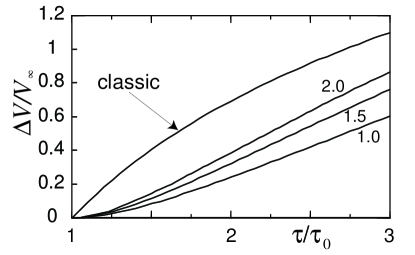
Figure 3: Rapidity spread vs. time for causal and classic diffusion computed using (27), (28) and (25) respectively. Causal curves are for $\tau_{o}/\tau_{d}=1$, 1.5, and 2. Rapidity spreads are divided by the value $2D_{o}/\tau_{o}=2\alpha/3$.

The width computed with varying coefficients increases without bound, albeit slowly. This behavior distinguishes (27) and (28) from the constant-coefficient widths obtained from (19) and (20). Nevertheless, the short time behavior shown in fig. 3 resembles the constant-coefficient case in fig. 2. In both cases the classic and causal results converge over longer times. Note that the results in fig. 3 are normalized to $2D/\tau_{o}=2/3\alpha$ using the value of $D$ at $\tau_{o}$.

To apply these results to collisions, we must specify the diffusion coefficient $D$ and the relaxation time $\tau_{d}$. Transport coefficients in quark gluon plasma and hadron matter have been been studied extensively Gavin85 ; Prakash ; PVW ; HeiselbergPethick ; Moore ; diffusion . Flavor and charge diffusion estimates in a plasma yield $D\sim 1-3$ fm and $\tau_{d}\sim 3D\sim 3-9$ fm HeiselbergPethick . The hadron gas case, which is more relevant to this work, is complicated by the menagerie of resonances produced in collisions. In ref. diffusion , the charge diffusion coefficient was computed using a hadronic transport model, yielding $D\approx 2$ fm and $\tau_{d}\approx 6$ fm.

We argue in sec. VI that the short time behavior in figs. 2 and 3 describes diffusion following hadronization. Hadrons form at a rather late time, roughly $\tau_{o}\sim 6-12$ fm. If freeze out occurs shortly thereafter, at $\tau_{f}$ less than 20 fm, then the range $\tau/\tau_{o}<3$ is important. A hadronic relaxation time $\tau_{d}\sim 6$ fm is relevant, so that $1<\alpha<2$. In this case causal diffusion gives a much slower spread in rapidity than classic diffusion.

IV Fluctuations and Correlations

Let us now turn to net charge fluctuations and their dissipation. To begin, we review key features of multiplicity and charge fluctuation observables. Our discussion builds on the detailed treatment in ref. PruneauGavinVoloshin , which stresses the relation of fluctuation observables to two-particle correlation functions. We extend that treatment by identifying the net-charge correlation function (34) that drives dynamic charge fluctuations. In the next section we will show how diffusion affects the evolution of this correlation function.

Dynamic fluctuations are generally determined from the measured fluctuations by subtracting the statistical value expected, e.g., in equilibrium PruneauGavinVoloshin . Dynamic multiplicity fluctuations are characterized by

$$R_{aa}={{\langle N^{2}\rangle-\langle N\rangle^{2}-\langle N\rangle}\over{\langle N\rangle^{2}}},$$ (29)

where $\langle\cdots\rangle$ here is the event average. This quantity is obtained from the multiplicity variance by subtracting its Poisson value $\langle N\rangle$. Similarly, the covariance for different species is

$$R_{ab}={{\langle N_{a}N_{b}\rangle-\langle N_{a}\rangle\langle N_{b}\rangle}\over{\langle N_{a}\rangle\langle N_{b}\rangle}},$$ (30)

which also vanishes for Poisson statistics. These quantities depend only on the two-body correlation function

$$r_{ab}(\eta_{1},\eta_{2})=\rho_{ab}(\eta_{1},\eta_{2})-\rho_{a}(\eta_{1})\rho_{b}(\eta_{2}),$$ (31)

where $\rho_{ab}(\eta_{1},\eta_{2})=dN_{ab}/d\eta_{1}d\eta_{2}$ is the rapidity density of particle pairs for species $a$ and $b$ at the respective pseudorapidities $\eta_{1}$ and $\eta_{2}$, and $\rho_{a}$ is the single particle rapidity density. We use the same symbol for momentum and configuration space rapidity, because we will take these quantities to be equal in later sections. In PruneauGavinVoloshin it is shown that

$$R_{ab}={{1}\over{\langle N_{a}\rangle\langle N_{b}\rangle}}\int\!d\eta_{1}d\eta_{2}\,r_{ab}(\eta_{1},\eta_{2}).$$ (32)

These quantities are robust in that they are normalized to minimize the effect of experimental efficiency and acceptance.

The STAR and CERES experiments characterize dynamic net-charge fluctuations using the robust variance

$$\nu\equiv R_{++}+R_{--}-2R_{+-},$$ (33)

proposed in PruneauGavinVoloshin ; here we use $\nu$ rather than the more conventional notation $\nu_{dyn}$ for simplicity. To establish the relation of $\nu$ to the net charge correlation function

$$q(\eta_{1},\eta_{2})=r_{++}+r_{--}-r_{+-}-r_{-+},$$ (34)

we integrate over a rapidity interval to find

$$N^{2}\Omega\equiv\int\!\!\!\int qd\eta_{1}d\eta_{2}=N(\omega_{q}-1),$$ (35)

where the variance of the net charge is $N\omega_{q}={\langle(N_{+}-N_{-})^{2}\rangle-\langle N_{+}-N_{-}\rangle^{2}}$ and the average number of charged particles is $N\equiv\langle N_{+}+N_{-}\rangle$. Expanding (35) yields

$$\Omega=f_{+}^{2}R_{++}+f_{-}^{2}R_{--}-2f_{+}f_{-}R_{+-},$$ (36)

where $f_{+}=\langle N_{+}\rangle/N=1-f_{-}$. If the average numbers of particles and antiparticles are nearly equal,

$$\nu\approx 4\Omega.$$ (37)

HIJING simulations show that this relation is essentially exact for mesons at SPS and RHIC energy (we find $\nu$ and $4\Omega$ are equal with 2% statistical error at SPS energy). We mention that $\Omega$ itself was suggested as an observable in ref. BowerGavin and that PHENIX measures the related quantity $\omega_{Q}=1+N\Omega$. However, $\Omega$ is not strictly robust. The next section implies that $q$ and, consequently, $\Omega$ is of more fundamental interest than $\nu$. However, in view of (37) and the qualitative aims of fluctuation studies, we will regard these quantities as interchangeable.

V Correlations and Diffusion

To understand how diffusion can dissipate dynamic fluctuations of the net charge and other conserved quantities, we apply the theoretical framework developed by Van Kampen and others VanKampen . A relativistic extension of these techniques will enable the computation of the correlation function (34) as well as statistical quantities like $\nu$, while introducing no additional parameters.

We start with a single charged species of conserved density $n(\mathbf{x},t)$ that evolves by diffusion. Consider an ensemble of events in which $n(\mathbf{x},t)$ is produced with different values at each point with probability $P\{n(\mathbf{x},t)\}$. After ref. VanKampen , one writes a master equation describing the rate of change of $P$ in terms of transition probabilities to states of differing $n$ on a discrete spatial lattice. Diffusion and flow are described as transitions in which particles “hop” to and from neighboring points. The Fokker-Planck formulation in ref. ShuryakStephanov can be obtained from this master equation in the appropriate limit. Alternatively, one can use the master equation to obtain a partial differential equation for the density correlation function by taking moments of $P$. The derivation is standard and we do not reproduce it here VanKampen .

If the one body density follows classic diffusion dynamics, then the density correlation function

$$r(\mathbf{x}_{1},\mathbf{x}_{2})\equiv\langle n_{1}n_{2}\rangle-\langle n_{1}\rangle\langle n_{2}\rangle-\delta(\mathbf{x}_{1}-\mathbf{x}_{2})\langle n_{1}\rangle,$$ (38)

satisfies the classic diffusion equation

$$\left({{\partial}\over{\partial t}}-D(\nabla_{1}^{2}+\nabla_{2}^{2})\right)r(\mathbf{x}_{1},\mathbf{x}_{2})=0$$ (39)

VanKampen . This density correlation function is analogous to rapidity-density correlation function (31). If the event-averaged single-particle density satisfies (1), then we can extend this result to causal diffusion by fourier transforming (39) and using (6), as in sec. II. The inverse transform yields

$$\left(\tau_{d}{{\partial^{2}}\over{\partial t^{2}}}+{{\partial}\over{\partial t}}-D(\nabla_{1}^{2}+\nabla_{2}^{2})\right)r(\mathbf{x}_{1},\mathbf{x}_{2})=0.$$ (40)

We remark that the delta-function term in (38) implies that the volume integral of $r$ vanishes when particle number fluctuations obey Poisson statistics. This term is derived along with (39) in ref. VanKampen ; it ensures that correlations vanish in global equilibrium.

In a nuclear collision with several charged species, only the net charge density $n^{+}-n^{-}$ satisfies diffusion dynamics, since chemical reactions can change one species into another. We define the net charge correlation function $q(\mathbf{x}_{1},\mathbf{x}_{2})$ as

$$q \equiv \langle(n_{1}^{+}-n_{1}^{-})(n_{2}^{+}-n_{2}^{-})\rangle-\langle n_{1}^{+}-n_{1}^{-}\rangle\langle n_{2}^{+}-n_{2}^{-}\rangle$$ (41)

$$-\delta(\mathbf{x}_{1}-\mathbf{x}_{2})\langle n_{1}^{+}+n_{1}^{-}\rangle.$$

Observe that the integral

$$\int qd\mathbf{x}_{1}d\mathbf{x}_{2} = \langle(N_{+}-N_{-})^{2}\rangle-\langle N_{+}-N_{-}\rangle^{2}$$ (42)

$$-\langle N_{+}+N_{-}\rangle$$

gives the net charge fluctuations minus its value for uncorrelated Poisson statistics. This integral vanishes in equilibrium. We expand (41) to write $q=r_{++}+r_{--}-r_{+-}-r_{-+}$, where each $r_{++}$ and $r_{--}$ has the form (38) and $r_{+-}\equiv\langle n_{1}^{+}n_{2}^{-}\rangle-\langle n_{1}^{+}\rangle\langle n_{2}^{-}\rangle$.

To obtain evolution equations for the matter produced in ion collisions, we incorporate longitudinal expansion following sec. III. The net-charge correlation function $q(\eta_{1},\eta_{2},\tau)$ is given by (34), where we now take

$$r_{ab}\equiv\langle\rho_{1}^{a}\rho_{2}^{b}\rangle-\langle\rho_{1}^{a}\rangle\langle\rho_{2}^{b}\rangle-\delta_{ab}\delta(\eta_{1}-\eta_{2})\langle\rho_{1}^{a}\rangle.$$ (43)

This correlation function has the same form as (41) with densities $n$ replaced by rapidity densities $\rho=dN/d\eta\propto n\tau$ and $\mathbf{x}_{1,2}$ replaced by spatial rapidities $\eta_{1,2}$. We find that $q(\eta_{1},\eta_{2},\tau)$ obeys

$$\left(\tau_{d}\frac{\partial^{2}}{\partial\tau^{2}}+\frac{\partial}{\partial\tau}-D(\nabla_{1}^{2}+\nabla_{2}^{2})\right)q=0$$ (44)

for $\nabla_{1,2}^{2}=\tau^{-2}\partial^{2}/\partial\eta_{1,2}^{2}$.

To compute the effect of diffusion on net charge fluctuations in the next section, we write (44) in terms of the relative rapidity $\eta_{r}\equiv\eta_{1}-\eta_{2}$ and average rapidity $\eta_{a}=(\eta_{1}+\eta_{2})/2$:

$$\left(\tau_{d}\frac{\partial^{2}}{\partial\tau^{2}}+\frac{\partial}{\partial\tau}-{{2D}\over{\tau^{2}}}{{\partial^{2}}\over{\partial\eta_{r}^{2}}}-{{D}\over{\tau^{2}}}{{\partial^{2}}\over{\partial\eta_{a}^{2}}}\right)q=0;$$ (45)

the “2” follows from the transformation to relative rapidity $\eta_{r}$. To compute the widths of $q(\eta_{r},\eta_{a},\tau)$ in relative or average rapidity, one multiplies (45) by $\eta_{r}^{2}$ or $\eta_{a}^{2}$ and integrates over both variables. We find

$$\Delta\langle(\eta_{r}-\langle\eta_{r}\rangle)^{2}\rangle=2\Delta{V}(\tau)$$ (46)

and

$$\Delta\langle(\eta_{a}-\langle\eta_{a}\rangle)^{2}\rangle=\Delta{V}(\tau),$$ (47)

where $\Delta{V}(\tau)$ is calculated using (20) (or (28) if a time-dependent $\tau_{d}$ and $D$ is more appropriate).

VI Survival of Signals

In this section we discuss how diffusion can affect our ability to interpret hadronization signals. As a concrete illustration, we suppose that collisions form a quark gluon plasma that hadronizes at a time $\tau_{o}$, producing anomalous dynamic charge fluctuations $\nu$. The hadronization model of Jeon and Koch JeonKoch implies that plasma produces a value $N\nu_{\rm qgp}\approx-3$. In contrast, the value for a hadronic resonance gas is variously estimated in the range from $N\nu\approx-1$ JeonKoch to $-1.7$ STAR . Hadronic diffusion from $\tau_{o}$ to a freeze out time $\tau_{f}$ can dissipate these fluctuations, reducing $|\nu|$.

We ask whether hadronic diffusion can plausibly bring plasma fluctuations near the hadron gas values. While the estimates of ref. JeonKoch can be questioned Bialas , they will serve here as benchmarks. In this section we emphasize the impact of causal diffusion on this problem, employing a simplified approach tailored to that aim. Phenomenological conclusions require a more realistic model.

Before proceeding, we emphasize that ref. JeonKoch compares quark gluon plasma and hadron gas fluctuations as they might emerge from distinct systems at equivalent chemical potential and temperature. In contrast, the fluctuations in a hadron gas that has evolved from a plasma initial state are fixed by charge conservation. Suppose that hadronization in single event produces a positive charge in one rapidity subinterval with a compensating negative charge in another. The final hadronic state maintains that situation – freezing in the plasma fluctuations – unless diffusion can redistribute the charges between those subintervals.

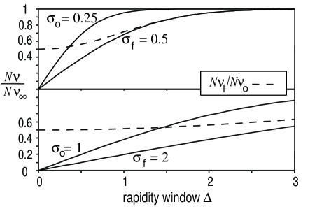
Figure 4: Rapidity dependence of dynamic charge fluctuations assuming diffusion has increased the width from $\sigma_{0}=1$ to $\sigma_{f}=2$ (bottom) and $\sigma_{0}=0.25$ to $\sigma_{f}=0.5$ (top).

To compute fluctuation observables following secs. III and V, we specify the correlation function by identifying spatial and momentum-space rapidity at a fixed freeze out proper time $\tau_{f}$. Observe that ISR and FNAL data Whitmore can be characterized as Gaussian near midrapidity. Moreover, these data show that charged particle correlations are functions of the relative rapidity $\eta_{r}=\eta_{1}-\eta_{2}$ with only a weak dependence on the average rapidity $\eta_{a}=(\eta_{1}+\eta_{2})/2$. Near midrapidity, these data inspire the form

$$q(\eta_{r},\eta_{a})\approx{{q_{o}}\over{2\pi\sigma\Sigma}}e^{-\eta_{r}^{2}/2\sigma^{2}-\eta_{a}^{2}/2\Sigma^{2}}$$ (48)

for $\Sigma\gg\sigma$. Diffusion increases the widths $\sigma$ and $\Sigma$ compared to their initial values $\sigma_{o}$ and $\Sigma_{o}$ at the hadronization time $\tau_{o}$ in accord with (46) and (47). For simplicity, we assume that $\Sigma_{o}$ is sufficiently large that we can neglect the time dependence of $\Sigma$ in (47). We point out that (48) is an exact solution of the classic diffusion equation on an infinite rapidity interval for Gaussian initial conditions. Moreover, (48) is a good approximation for causal diffusion, provided that the rapidity region of interest does not appreciably exceed $\sigma$ or $\Sigma$; see the discussion in sec. II.

Dynamic fluctuations $\nu$ are computed by integrating $q$ over an interval $-\Delta/2\leq\eta_{1},\,\eta_{2}\leq\Delta/2$ corresponding to the experimental acceptance. For $\Sigma$ greater than $\Delta/2$ and $\sigma$, we use (35) and (37) to estimate $\nu$

$$N\nu \approx {{4}\over{N}}\int_{-\Delta/2}^{\Delta/2}\int_{-\Delta/2}^{\Delta/2}q(\eta_{1},\eta_{2})d\eta_{1}d\eta_{2}$$ (49)

$$\approx {{8}\over{N}}\int_{0}^{\Delta/2}d\eta_{a}\int_{-\Delta/2+\eta_{a}}^{\Delta/2-\eta_{a}}q(\eta_{r},\eta_{a})d\eta_{r}$$

$$\approx {N\nu}_{{}_{\infty}}\,{\rm erf}\left(\Delta/\sqrt{8}\sigma\right),$$

where the total number of charged particles is $N\approx 2\rho\Delta$. We take the rapidity density $\rho$ for each charge species to be uniform. The quantity $N\nu_{{}_{\infty}}=2q_{o}(2\pi\rho^{2}\Sigma^{2})^{-1/2}$ is the value obtained for a large rapidity window.

The dependence of the dynamic fluctuations $N\nu$ on the relative rapidity interval $\Delta$ implied by (49) is shown in fig. 4 for several ad hoc values of $\sigma$. Also shown as dashed curves are the ratios of these quantities,

$${{N\nu_{f}}\over{N\nu_{o}}}={{{\rm erf}\left(\Delta/\sqrt{8}\sigma_{f}\right)}\over{{\rm erf}\left(\Delta/\sqrt{8}\sigma_{o}\right)}},$$ (50)

computed for $\sigma_{o}$ the smaller initial width and $\sigma_{f}$ the larger final width. This ratio indicates how much the fluctuations are reduced as the width increases from $\sigma_{o}$ to $\sigma_{f}$. In both figures, the change in widths are chosen so that they nearly “hide” initial QGP fluctuations at the level expected in ref. JeonKoch , since $N\nu_{\rm hg}/N\nu_{\rm qgp}\approx 1/3-1/2$. Balance function measurements are consistent with a width $\sigma\approx 0.5$ Mitchell . ISR and FNAL experiments suggest $\sigma\approx 1$ in pp collisions.

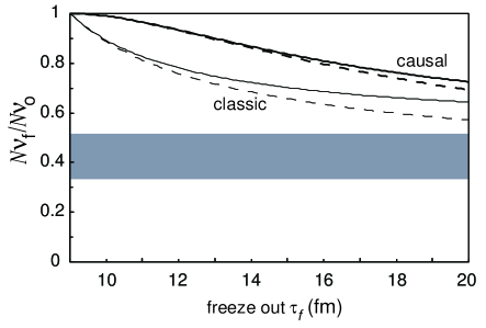
Figure 5: Decrease in dynamic charge fluctuations as a function of freeze out time $\tau_{f}$ for the acceptance $\Delta=1$ and $\sigma_{0}=0.25$. The gray band indicates the level needed to obscure plasma signals. Solid and dashed curves are respectively computed for constant and varying coefficients using (20) and (28) and the corresponding classic eqs. (19) and (25).

The question then becomes: are such increases in $\sigma$ plausible in a diffusion model? Equation (46) implies that $\sigma_{f}^{2}=\sigma_{o}^{2}+2\Delta{V}(\tau_{f})$. The relevant “formation time” is the time at which hadronization occurs. This occurs quite late in the evolution, roughly from $\tau_{o}\sim 6$ to 12 fm. Freeze out occurs later, perhaps as late as $\tau_{f}\sim 20$ fm. The ratio $\tau_{f}/\tau_{0}$ is then in the range from one to two, where the difference between causal and classic diffusion is substantial, as shown in figs. 2 and 3. We take $D\approx 2$ fm and $\tau_{d}\approx 6$ fm from ref. diffusion , as discussed in sec. III.

The solid curves in fig. 5 show the decrease of dynamic fluctuations computed using (50), (46), and (20). The dashed curves are computed using (28) instead of (20). We take the value $\sigma_{o}\approx 0.25$ for the initial width; larger values imply a smaller net reduction of $N\nu$. A hadronization time $\tau_{o}=9$ fm is assumed, corresponding to $\alpha=\tau_{o}/\tau_{d}=1.5$ in figs. 2 and 3. The gray band indicates the level to which $N\nu$ must be reduced to hide the effect of plasma fluctuations. We see that classic diffusion can bring $N\nu$ to this level if the system lives as long as 20 fm, while causal diffusion cannot.

VII Summary

In this paper we introduce a causal diffusion equation to describe the relativistic evolution of net charge and other conserved quantities in nuclear collisions. We find that causal limitations inhibit dissipation. To study the effect of this dissipation on fluctuation signals, we obtain a causal diffusion equation for the two-body correlation function. Our approach complements the treatment in ShuryakStephanov , but is more easily generalized to include radial flow and other dynamic effects for comparison to data.

We then use these equations to provide estimates that show that net charge fluctuations induced by quark gluon plasma hadronization can plausibly survive diffusion in the hadronic stage. This result bolsters our optimism for fluctuation and correlation probes of hadronization and other interesting dynamics. Our aim here has been to emphasize the impact of causal diffusion on charge fluctuations. Correspondingly, we employ an idealized approach tailored to that aim. Phenomenological conclusions require a more realistic model, to be developed elsewhere.

Our results on post-hadronization diffusion owe to the similarity of the lifetime of the hadronic system and the relaxation time for diffusion $\tau_{d}$. In fact, RHIC data suggests hadronic lifetimes that are as short or shorter than we assume: HBT Lisa and resonance Markert measurements suggest a lifetime from roughly $5$ to $10$ fm. On the other hand, our estimate of $\tau_{d}$ rests on transport calculations in ref. diffusion . The importance of this problem invites further study of charge and other transport coefficients.

In closing, we briefly comment on the experimental situation. Charge fluctuation measurements give roughly similar values from SPS to RHIC energy Mitchell . Furthermore, the STAR experiment finds $N\nu\approx-1.5$ at RHIC STAR . While this value is close to the benchmark hadron gas estimates JeonKoch ; STAR , we emphasize that those estimates were constructed for an equilibrium resonance gas assuming no prior plasma stage. Flow and jet quenching measurements provide strong indications – if not proof – of plasma formation Miklos . As discussed earlier, $N\nu$ can be very different in a resonance gas formed from a hadronizing partonic system and, indeed, should be very close to plasma values.

Extraordinary charge fluctuations should be seen, but are not. It may be that net-charge fluctuations produced by plasma hadronization are closer to the benchmark hadronic estimates, as suggested by Bialas Bialas . What then? Experimentally, one can turn to the centrality and azimuthal-angle dependence of fluctuations and, eventually, to correlation-function measurements as more sensitive probes of net charge fluctuations. Such studies have already begun to yield important information Mitchell ; Gavin04 . In addition, one can study baryon number and isospin fluctuations, which are more closely related to the QCD order parameter and, therefore, to hadronization physics and phase transition dynamics RajagopalShuryakStephanov ; BowerGavin .

References

- (1) J. T. Mitchell [PHENIX], Proc. Quark Matter 2004, to be published J. Phys. G. (2004) arXive:nucl-ex/0404005; G. Westfall [STAR] ibid, arXive:nucl-ex/0404004; C. Pruneau [STAR], arXiv:nucl-ex/0401016.
- (2) G. Baym, G. Friedman and I. Sarcevic, Phys. Lett. B219, (1989) 205; M. Gazdzicki and S. Mrowczynski, Z. Phys. C54 (1992) 127; H. Heiselberg, Phys. Rept. 351 (2001) 161; S. Y. Jeon and V. Koch, arXiv:hep-ph/0304012.
- (3) M. Stephanov, K. Rajagopal and E. V. Shuryak, Phys. Rev. D 60, 114028 (1999) [hep-ph/9903292].
- (4) M. Asakawa, U. Heinz, B. Müller, Phys. Rev. Lett. 85, 2072 (2000); S. Jeon and V. Koch,ibid, 2076; V. Koch, M. Bleicher, S. Jeon, Nucl. Phys. A698 (2002) 261.
- (5) D. Bower and S. Gavin, Phys. Rev. C 64 051902 (2001); Y. Hatta and M. A. Stephanov, Phys. Rev. Lett. 91, 102003 (2003); Erratum, ibid 91 129901 (2003).
- (6) E. V. Shuryak and M. A. Stephanov, Phys. Rev. C 63, 064903 (2001) [arXiv:hep-ph/0010100].
- (7) A. Muronga, Phys. Rev. Lett. 88, 062302 (2002); Phys. Rev. C 69, 034903 (2004).
- (8) D. Teaney, arXiv:nucl-th/0403053.
- (9) M. Abdel Aziz and S. Gavin, Proc. 19th Winter Workshop on Nuclear Dynamics, Breckenridge, Colorado, USA, February 8-15, 2003, (EP Systema Bt., Debrecen, Hungary, 2003), 159.
- (10) N. G. Van Kampen, Stochastic Processes in Physics and Chemistry, (Elsevier Science, Amsterdam, 1997); C. W. Gardiner, Handbook of Stochastic Methods for Physics, Chemistry and the Natural Sciences, (Springer, Berlin, 2002).
- (11) C. Cataneo, Atti Semin. Mat. Fis. Univ. Modena 3, 3 (1948); P. Vernotte, C. R. Acad. Sci. Paris 246, 3154 (1958).
- (12) H. Grad, Comm. Pure Appl. Math. 2, 331 (1949).
- (13) W. Israel and J. M. Stewart, Ann. Phys. (N.Y.) 118, 341 (1979).
- (14) E. Zauderer, Partial Differential Equations of Applied Mathematics, 2nd ed. (Wiley, New York, 1989).
- (15) D. D. Joseph and L. Preziosi, Rev. Mod. Phys. 61, 41 (1989).
- (16) S. Gavin, Nucl. Phys. A 435, 826 (1985).
- (17) D. M. Forster, Hydrodynamic fluctuations, Broken symmetry, and Correlation Functions, (Benjamin, New York, 1975).
- (18) C. Manuel and S. Mrowczynski, arXiv:hep-ph/0403054.
- (19) M. Prakash, M. Prakash, R. Venugopalan and G. Welke Phys. Rept. 227, 321 (1993).
- (20) A. Muronga, Phys. Rev. C 69, 044901 (2004).
- (21) H. Heiselberg, C.J. Pethick Phys. Rev. D48, 2916, (1993).
- (22) Peter Arnold, Guy D. Moore, and Lawrence G. Yaffe, JHEP 0305, 051, (2003) [arXiv:hep-ph/0302165].
- (23) N. Sasaki, O. Miyamura, S. Muroya and C. Nonaka, Europhys. Lett. 54, 38 (2001) [arXiv:hep-ph/0007121].
- (24) S. R. de Groot, H. A. van Leeuven and C. G. van Weert, Relativistic Kinetic Theory, (North Holland, Amesterdam, 1980).
- (25) J. D. Bjorken, Phys. Rev. D 27, 140 (1983).
- (26) S. Gavin, Nucl. Phys. B 351, 561 (1991).
- (27) C. Pruneau, S. Gavin and S. Voloshin, Phys. Rev. C 66, 044904 (2002) [arXiv:nucl-ex/0204011].
- (28) J. Adams et al. [STAR], Phys. Rev. C bf 68, 044905 (2003).
- (29) A. Bialas, Phys. Lett. B 532, 249 (2002) [arXiv:hep-ph/0203047].
- (30) J. Whitmore, Phys. Rept. 27, 187 (1976); L. Foa, Physics Reports, 22, 1( 1075); H. Boggild and T. Ferbel, Ann. Rev. Nucl. Part. Sci. 24, 451 (l974).
- (31) S. A. Bass, P. Danielewicz and S. Pratt, Phys. Rev. Lett. 85, 2689 (2000) [arXiv:nucl-th/0005044].
- (32) M. Lisa [STAR], Acta Phys. Polon. B35, 37 (2004).
- (33) C. Markert [STAR], arXiv:nucl-ex/0404003.
- (34) M. Gyulassy, arXiv:nucl-th/0403032.
- (35) S. Gavin, Phys. Rev. Lett., to be published (2004) [arXiv:nucl-th/0308067]; J. Phys. G., to be published; [arXiv:nucl-th/0404048].