Study of a possible $S=+1$ dynamically generated baryonic resonance

Abstract

Starting from the lowest order chiral Lagrangian for the interaction of the baryon decuplet with the octet of pseudoscalar mesons we find an attractive interaction in the $\Delta K$ channel with $L=0$ and $I=1$, while the interaction is repulsive for $I=2$. The attractive interaction leads to a pole in the second Riemann sheet of the complex plane and manifests itself in a large strength of the $\Delta K$ scattering amplitude close to the $\Delta K$ threshold, which is not the case for $I=2$. However, we also make a study of uncertainties in the model and conclude that the existence of this pole depends sensitively upon the input used and can disappear within reasonable variations of the input parameters. We take advantage to study the stability of the other poles obtained for the $\frac{3}{2}^{-}$ dynamically generated resonances of the model and conclude that they are stable and not contingent to reasonable changes in the input of the theory.

1 Introduction

The dynamical generation of baryonic resonances within a chiral unitary approach has experienced much progress from early works which generated the $\Lambda(1405)$ [1, 2]. Further studies unveiled other dynamically generated resonances which can be associated to known resonances and others found new states [3, 4, 5]. Recently, it has been shown that there are actually two octets and a singlet of dynamically generated $J^{P}=1/2^{-}$ resonances, which include among others two $\Lambda(1405)$ states, the $\Lambda(1670)$, the $\Sigma(1650)$ and a possible $I=1$ state close to the $K^{-}p$ threshold [3, 6, 7].

What we call dynamically generated resonances are states which appear in a natural way when studying the meson baryon interaction using coupled channel Bethe-Salpeter equations (or equivalent unitary schemes) with a kernel (potential) obtained from the lowest order chiral Lagrangian. This subtlety is important since higher order Lagrangians sometimes contain information on genuine resonances, and unitary schemes like the Inverse Amplitude Method (IAM) [8, 9] make them show up clearly, giving the appearance that they have been generated dynamically, when in fact they were already hidden in the higher order Lagrangian. This is the case of the vector mesons in the pseudoscalar meson-meson interaction, which are accounted for in the ${\cal L}^{(4)}$ Lagrangian of Gasser and Leutwyler [10] among other interactions. This is shown in [11] where assuming explicit vector meson exchange and also scalar meson exchange the values of the $L_{i}$ coefficients of [10] can be reproduced. The introduction of the term genuine resonance, as opposed to dynamically generated, finds its best definition within the context of the large $N_{c}$ counting. In the limit of large $N_{c}$ there are series of resonances which appear [11, 12] which we call genuine resonances. In this limit the loops that characterize the series of the Bethe-Salpeter equation vanish and the dynamically generated resonances fade away [13]. The genuine resonances cannot be generated dynamically and then this establishes a distinction between the different resonances, the nature of which can be distinguished when looking at the evolution of the poles as we gradually make $N_{c}$ large. This exercise in the meson-meson interaction [13, 14] shows that the $\sigma(500)$, $f_{0}(980)$, $a_{0}(980)$ scalar resonances are dynamically generated and disappear in the large $N_{c}$ limit, while the $\rho$, $K^{*}$ remain in this limit. These findings would not alter the philosophy of ref. [11], making the exchange of vector mesons and scalar mesons responsible for the $L_{i}$ coefficients, but the choice of the particles exchanged, in the sense that the scalar mesons to be used there should not be the lowest lying ones mentioned above, but the nearest ones in energy in the Particle Data Book (PDB)[15].

Coming back to the meson baryon case, this distinction holds equally and there are some resonances which are dynamically generated from the meson-baryon interaction, solving the Bethe-Salpeter equations in coupled channels, while there are others (the large majority) which do not qualify as such and stand, hence, as genuine resonances. From the point of view of constituent quarks, the latter ones would basically correspond to $3q$ states, while the former ones would qualify more like meson baryon quasibound states or meson baryon molecules.

So far, in the light quark section, the dynamically generated baryon resonances have been found only in the interaction of the octet of stable baryons with the octet of pseudoscalar mesons in $L=0$, leading to $J^{P}=1/2^{-}$ [3, 4, 6, 7] and in the interaction of the decuplet of baryons with the octet of pseudoscalar mesons in $L=0$, leading to $J^{P}=3/2^{-}$ states [16].

The chiral unitary approach is purely a theoretical tool to describe from scratch the interaction of mesons with baryons. If one uses as input only the contact Weinberg-Tomozawa interaction between the mesons and baryon as we do, the interaction is fixed and there is only a free parameter, the cut-off in the loop, or a subtraction constant in the dispersion relation integral, which is fitted to a piece of data. However, this cut-off or subtraction constant should be of natural size [3]. After that the theory makes predictions for meson baryon amplitudes and some times a pole appears indicating one has generated a resonance, which was not explicitly put into the scheme. These are the dynamically generated resonances. Most of the resonances listed in the PDB can not be generated in this way indicating they are genuine and not dynamically generated. Trivial examples of genuine resonances would be the decuplet of baryons to which the $\Delta(1232)$ belongs.

With current claims about the $\Theta^{+}$ pentaquark [17] and the extensive work to try to understand its nature [18, 19] (see refs. [20, 21] for a list of related references), one is immediately driven to test whether such a state could qualify as a dynamically generated resonance from the $KN$ interaction, but with a basically repulsive $KN$ interaction from the dominant Weinberg-Tomozawa Lagrangian this possibility is ruled out.

In view of that, the possibility that it could be a bound state of $K\pi N$ was soon suggested [22], but detailed calculations using the same methods and interaction that lead to dynamically generated mesons and baryons indicate that it is difficult to bind that system with natural size parameters [23].

More recently some new steps have been done in the chiral symmetry approach introducing the interaction of the $\Delta$ and the other members of the baryon decuplet with the pion and the octet partners. In this sense, in [16] the interaction of the decuplet of $3/2^{+}$ baryons with the octet of pseudoscalar mesons is shown to lead to many states that have been associated to experimentally well established resonances. Also, in ref. [16] a comment was made that maybe a resonance could be generated with exotic quantum numbers in the 27 representation of $SU(3)$ . The purpose of the present paper is to elaborate upon this idea studying the possible existence of a pole in this exotic channel as well as the uncertainties and stability of the results.

In the present work we show that the interaction of the $3/2^{+}$ baryon decuplet with the $0^{-}$ meson octet leads to a state of positive strangeness, with $I=1$ and $J^{P}=3/2^{-}$, hence, an exotic baryon in the sense that it cannot be constructed with only three quarks. This would be the first reported case of a dynamically generated baryon with positive strangeness. However, we study the stability of the results with reasonable changes of the input parameters and realize that the results are unstable and the pole disappears within reasonable assumptions. The situation remains unclear concerning this pole. In view of that we have also reviewed the situation for the rest of the dynamically generated $3/2^{-}$ resonances of the model and we find that they are stable and their properties are quite independent of these changes in the input of the theory.

2 Formulation

The lowest order chiral Lagrangian for the interaction of the baryon decuplet with the octet of pseudoscalar mesons is given by [24]

$${\cal L}=-i\bar{T}^{\mu}{\cal D}\!\!\!\!/T_{\mu}$$ (1)

where $T^{\mu}_{abc}$ is the spin decuplet field and ${\cal D}^{\nu}$ the covariant derivative given by

$${\cal D}^{\nu}T^{\mu}_{abc}=\partial^{\nu}T^{\mu}_{abc}+(\Gamma^{\nu})^{d}_{a}T^{\mu}_{dbc}+(\Gamma^{\nu})^{d}_{b}T^{\mu}_{adc}+(\Gamma^{\nu})^{d}_{c}T^{\mu}_{abd}$$ (2)

where $\mu$ is the Lorentz index, $a,b,c$ are the $SU(3)$ indices and $\Gamma^{\nu}$ is the vector current given by

$$\Gamma^{\nu}=\frac{1}{2}(\xi\partial^{\nu}\xi^{\dagger}+\xi^{\dagger}\partial^{\nu}\xi)$$ (3)

with

$$\xi^{2}=U=e^{i\sqrt{2}\Phi/f}$$ (4)

where $\Phi$ is the ordinary 3$\times$3 matrix of fields for the pseudoscalar mesons [10] and $f$ is the pion decay constant, $f=93$ MeV. For the $s$-wave interaction some simplifications are possible in the algebra of the Rarita-Schwinger fields $T_{\mu}$ [25]. We write $T_{\mu}$ as $Tu_{\mu}$ where $u_{\mu}$ stands for the Rarita-Schwinger spinor which is given by [25, 26]

$$u_{\mu}=\sum_{\lambda,s}{\cal C}(1~{}\frac{1}{2}~{}\frac{3}{2}\ ;\ \lambda~{}s~{}s_{\Delta})\ e_{\mu}(p,\lambda)\ u(p,s)$$ (5)

with $e_{\mu}=(0,\hat{e})$ in the particle rest frame, $\hat{e}$ the spherical representation of the unit vector $(\lambda=0,\pm 1)$, ${\cal C}$ the Clebsch Gordan coefficients and $u(p,s)$ the ordinary Dirac spinors $(s=\pm\frac{1}{2})$. Then eq. (1) involves the Dirac matrix elements

$$\bar{u}(p^{\prime},s^{\prime})\gamma^{\nu}\ u(p,s)=\delta^{\nu 0}\delta_{ss^{\prime}}+{\cal O}(|\vec{p}|/M)$$ (6)

which for the $s$-wave interaction can be very accurately substituted by the non-relativistic approximation $\delta^{\nu 0}\delta_{ss^{\prime}}$ as done in [2] and related works. The remaining combination of the spinors $u_{\mu}u^{\mu}$ involves

$$\sum_{\lambda^{\prime},s^{\prime}}\sum_{\lambda,s}{\cal C}(1~{}\frac{1}{2}~{}\frac{3}{2}\ ;\ \lambda^{\prime}~{}s^{\prime}~{}s_{\Delta})\ e^{*}_{\mu}(p^{\prime},\lambda^{\prime})\ {\cal C}(1~{}\frac{1}{2}~{}\frac{3}{2}\ ;\ \lambda~{}s~{}s_{\Delta})\ e^{\mu}(p,\lambda)\ \delta_{ss^{\prime}}=-1+{\cal O}(|\vec{p}|^{2}/M^{2})~{}.$$ (7)

As one can see, at this point one is already making a nonrelativistic approximation and consistently with this, the decuplet states will be treated as ordinary nonrelativistic particles in what follows, concerning the propagators, etc. However, while making these nonrelativistic assumptions in the Lagrangian we shall keep the exact relativistic energies in the propagators. This small inconsistency is assumed in order to find a compromise between simplicity of the formalism and respecting accurately the thresholds of the reactions and the exact unitarity.

The interaction Lagrangian for decuplet-meson interaction can then be written in terms of the matrix

$$(\bar{T}\cdot T)_{ad}=\sum_{b,c}\bar{T}^{abc}T_{dbc}$$ (8)

as

$${\cal L}=3iTr\{\bar{T}\cdot T\,\,\,\Gamma^{0T}\}$$ (9)

where $\Gamma^{0T}$ stands for the transposed matrix of $\Gamma^{0}$, with $\Gamma^{\nu}$ given, up to two meson fields, by

$$\Gamma^{\nu}=\frac{1}{4f^{2}}(\Phi\partial^{\nu}\Phi-\partial^{\nu}\Phi\Phi).$$ (10)

For the identification of the $SU(3)$ components of $T$ to the physical states we follow ref. [27]:

$T^{111}=\Delta^{++}$, $T^{112}=\frac{1}{\sqrt{3}}\Delta^{+}$, $T^{122}=\frac{1}{\sqrt{3}}\Delta^{0}$, $T^{222}=\Delta^{-}$, $T^{113}=\frac{1}{\sqrt{3}}\Sigma^{*+}$, $T^{123}=\frac{1}{\sqrt{6}}\Sigma^{*0}$, $T^{223}=\frac{1}{\sqrt{3}}\Sigma^{*-}$, $T^{133}=\frac{1}{\sqrt{3}}\Xi^{*0}$, $T^{233}=\frac{1}{\sqrt{3}}\Xi^{*-}$, $T^{333}=\Omega^{-}$.

Hence, for a meson of incoming (outgoing) momenta $k(k^{\prime})$ we obtain the transition amplitudes, as in [2],

$$V_{ij}=-\frac{1}{4f^{2}}C_{ij}(k^{0}+k^{{}^{\prime}0}).$$ (11)

For strangeness $S=1$ and charge $Q=3$ there is only one channel $\Delta^{++}K^{+}$ which has $I=2$. For $S=1$ and $Q=2$ there are two channels $\Delta^{++}K^{0}$ and $\Delta^{+}K^{+}$ that we call channels 1 and 2, for which eq. (9) gives $C_{11}=0$, $C_{12}=C_{21}=-\sqrt{3}$, $C_{22}=-2$. From these one can extract the transition amplitudes for the $I=2$ and $I=1$ combinations and we find

$$V(S=1,I=2)=\frac{3}{4f^{2}}(k^{0}+k^{{}^{\prime}0});~{}~{}~{}~{}~{}V(S=1,I=1)=-\frac{1}{4f^{2}}(k^{0}+k^{{}^{\prime}0}).$$ (12)

These results indicate that the interaction in the $I=2$ channel is repulsive while it is attractive in $I=1$. There is a link to the $SU(3)$ representation since we have the decomposition

$$8\otimes 10=8\oplus 10\oplus 27\oplus 35$$

and the state with $S=1,\ I=1$ belongs to the 27 representation while the $S=1,\ I=2$ belongs to the 35 representation. As noted in [16] the interaction is attractive in the 8, 10 and 27 representations and repulsive in the 35. Indeed the strength of the interaction in those channels is proportional to 6, 3, 1 and –3. The attractive potential in the case of $I=1$ and the physical situation are very similar to those of the $\bar{K}N$ system in $I=0$, where the interaction is also attractive and leads to the generation of the $\Lambda(1405)$ resonance [1, 2, 3, 5]. The use of $V$ of eq. (11) as the kernel of the Bethe Salpeter equation [2], or the N/D unitary approach of [3] both lead to the scattering amplitude in the coupled channels

$$t=(1-VG)^{-1}V$$ (13)

although in the cases of eq. (12) we have only one channel for each $I$ state. In eq. (13), $V$ factorizes on shell [2, 3] and $G$ stands for the loop function of the meson and baryon propagators, the expressions for which are given in [2] for a cut off regularization and in [3] for dimensional regularization.

3 Results and Discussion

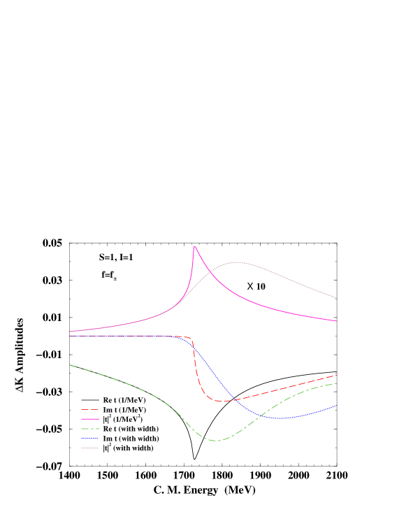
Figure 1: Amplitudes for $\Delta K\rightarrow\Delta K$ for $I=1$ with $f=f_{\pi}$.

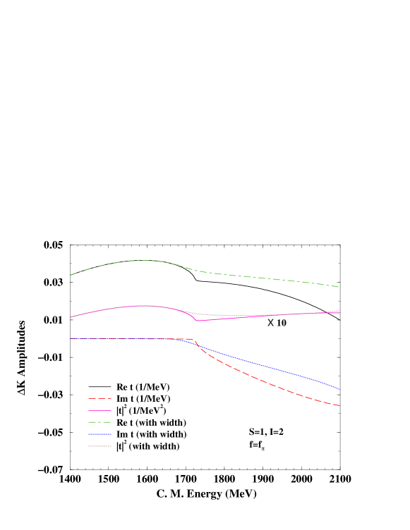
Figure 2: Amplitudes for $\Delta K\rightarrow\Delta K$ for $I=2$ with $f=f_{\pi}$.

The first thing we have to do is to fix the scale of regularization in the loop functions $G_{l}$ of eq. (6) of [4]. The criterion for that is given in [3] where dimensional regularization is used and $G_{l}$ depends upon a subtraction constant, $a_{l}$, that should have ’natural size’. Values of $a_{l}$ around $-2$ were found reasonable in [3] since they are equivalent to using cut off regularization with $q_{max}$ around 700 MeV [3]. In this latter reference, the authors established the equivalence between the dimensional regularization and a cut off method in which the $q^{0}$ integration in the loops is done analytically and the cut off is put in the three momentum $\vec{q}$. Thus, both regularization methods respect the basic symmetries of the problem. Details on the two methods and related formulae used can be seen in ref. [28] where a general study of the dynamically generated $3/2^{-}$ resonances is done. Here we study in detail the case of $S=1$, given the repercussion that such an exotic dynamically generated resonance would have.

We set up the value of $a_{l}$ or equivalently $q_{max}$ by fixing the poles for the resonances which appear more cleanly in [16, 28]. They are one resonance in $(I,S)=(0,-3)$, another one in $(I,S)=(1/2,-2)$ and another one in $(I,S)=(1,-1)$. The last two appear in [16] around 1800 MeV and 1600 MeV and they are identified with the $\Xi(1820)$ and $\Sigma(1670)$. We obtain the same results as in [16] using $a_{l}=-2$ or, equivalently, a cut off $q_{max}=700$ MeV. There are other peaks of the speed plot in [16], which we also reproduce, but they appear just at the threshold of some channels and stick there even when the cut off is changed. Independently of the meaning of these peaks, they can not be used to fix the scale of regularization.

With this subtraction constant we explore the analytical properties of the amplitude for $S=1$, $I=1$ in the first and second Riemann sheets. Firstly, we see that there is no pole below threshold in the first Riemann sheet as it would be in the case of a bound state. However, if we increase the cut off to 1.5 GeV (or, equivalently, $a_{l}=-2.9$ with $\mu=700$ MeV) we find a pole below threshold corresponding to a $\Delta K$ bound state. But this cut off or subtraction constant does not reproduce the position of the resonances discussed above.

Next we explore the second Riemann sheet. This is done using dimensional regularization setting the scale $\mu$ equal to $q_{max}=700$ MeV and the subtraction constant $a$ to $-2$ and changing $\bar{q}_{l}$ to $-\bar{q}_{l}$ in the analytical formula of $G_{l}$ in [4]. This procedure is equivalent to taking

$$G^{2nd}=G+2i\,\frac{p_{CM}}{\sqrt{s}}\,\frac{M}{4\pi}$$ (14)

with the variables on the right hand side of the equation evaluated in the first (physical) Riemann sheet. In the above equation $p_{CM}$, $M$ and $\sqrt{s}$ denote the CM momentum, the $\Delta$ mass and the CM energy respectively. With both methods we find a pole around $\sqrt{s}=1600$ MeV in the second Riemann sheet. This should have some repercussion on the physical amplitude as we show below.

The situation in the scattering matrix is revealed in figs. 1 and 2 which show the real and imaginary parts of the $\Delta K$ amplitudes for the case of $I=1$ and $I=2$ respectively. Using the cut off discussed above we can observe the differences between $I=1$ and $I=2$. For the case of $I=2$ the imaginary part follows the ordinary behaviour of the opening of a threshold, growing smoothly from threshold. The real part is also smooth, showing nevertheless the cusp at threshold. For the case of $I=1$, instead, the strength of the imaginary part is stuck to threshold as a reminder of the existing pole in the complex plane, growing very fast with energy close to threshold. The real part has also a pronounced cusp at threshold, which is also tied to the same singularity.

We have also done a more realistic calculation taking into account the width of the $\Delta$ in the intermediate states. For this we use the cut off method of regularization with $G$ given in [4] for stable intermediate particles. The width of the $\Delta$ is taken into account by adding $-i\Gamma(q^{2})/2$ to the $\Delta$ energy, $E_{l}(\vec{q})$, in the loop function $G_{l}$ of eq. (6) of ref [4] with $\Gamma(q^{2})$ given by

$$\Gamma(q^{2})=\Gamma_{0}\,\frac{q_{CM}^{3}}{\bar{q}_{CM}^{3}}\,\,\Theta(\sqrt{q^{2}}-M_{N}-m_{\pi})$$ (15)

where $q_{CM}$ and $\bar{q}_{CM}$ denote the momentum of the pion (or nucleon) in the rest frame of the $\Delta$ corresponding to invariant masses $\sqrt{q^{2}}$ and $M_{\Delta}$ respectively. In the above equation $\Gamma_{0}$ is taken as 120 MeV. The results are also shown in figs. 1 and 2 and we see that the peaks around threshold become smoother and some strength is moved to higher energies. Even then, the strength of the real and imaginary parts in the $I=1$ are much larger than for $I=2$. The modulus squared of the amplitudes shows some peak behavior around 1800 MeV in the case of $I=1$, while it is small and has no structure in the case of $I=2$.

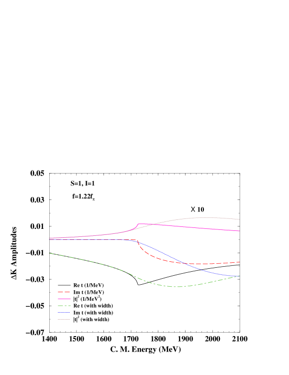
Figure 3: Amplitudes for $\Delta K\rightarrow\Delta K$ for $I=1$ with $f=f_{K}$.

The situation in figs. 1 and 2 is appealing but before proceeding further we would like to pay some attention to the stability of the results. So far we have used a unique meson decay constant, the one of the pion, $f=f_{\pi}=93$ MeV. One source of $SU(3)$ breaking in the problem comes from the renormalization of the meson decay constants which leads to different values of $f$ for the $\pi$, $K$ and the $\eta$ [10]. We thus repeat the calculations using $f_{K}=1.22f_{\pi}$. Yet, when doing this, we would like to change simultaneously the cut off such that we still obtain the poles for the $\Xi(1820)$ and $\Sigma(1670)$ (which also involve mainly the $K$ in their coupled channels). We repeat the calculations with $q_{max}$=800 MeV and the results are shown in figs. 3 and 4. We see in fig. 3 that the cusp effect is very much diminished with respect to the former set of parameters and the final cross section is decreased by about a factor of three. Compared to the cross section for $I=2$, shown in fig. 4, the cross section in $I=1$ is still bigger and grows faster but the effects are certainly less spectacular than before.

The weak signal in the case of fig. 3 reflects the fact that that in this case we do not find a pole in the second Riemann sheet. The interaction, which is a factor 6 weaker than in the octet case, as we mentioned above, and barely supported a pole when using $f=f_{\pi}$, becomes now too weak due to the $f^{-2}$ behaviour of the kernel (eq. 11) and the pole fades away.

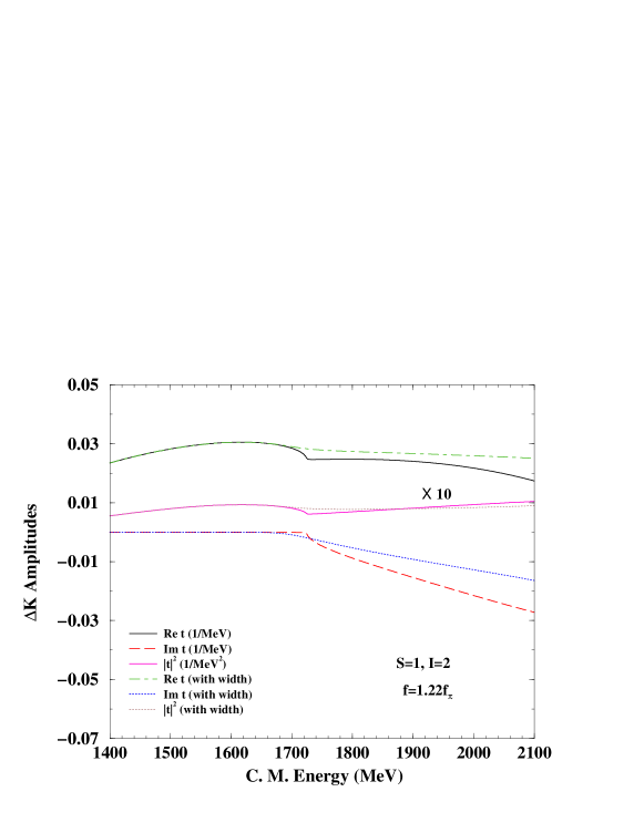
Figure 4: Amplitudes for $\Delta K\rightarrow\Delta K$ for $I=2$ with $f=f_{K}$.

In this exploratory investigation we should also mention that if $f$ is decreased by about $25\%$ with respect to $f_{\pi}$ we do find a pole in the first Riemann sheet just below the $\Delta K$ threshold indicating a bound state, something also mentioned in [16]. We have also studied the results making small changes in the mass of the $K$. Results depend weakly on the $K$ mass but qualitatively we find that increasing the $K$ mass the interaction becomes stronger (see eq. 11) and it is easier to find the pole, and vice versa.

We are thus in the border line between having and not having a pole, or in other words, the amplitudes are very sensitive to changes in the input parameters. We can not draw strong conclusions in this case since improvements in the theory could move the balance to one side or the other.

The former comment is in place since a more refined model should also contain extra channels which have been omitted here. These channels would be states made of a vector meson and a stable baryon which would also couple in $s$-wave, the $K^{*}N$ in the present case. These extra channels are expected to be relatively unimportant in the case of the other $3/2^{-}$ dynamically generated resonances [16, 28], because the Weinberg-Tomozawa interaction is six times, or three times larger, for the octet or decuplet representations respectively, than the present one which belongs to the 27 representation. So, in the present case where we look for the $\Delta K$ pole, the strength of the $\Delta K$ interaction is rather weak, and the effect of the other coupled channels and their interaction could alter substantially the results. We do not have at hand the theoretical tools to study the mixing of these channels and hence it is not possible presently to draw any other conclusions than the fact that the existence of the $\Delta K$ pole in $I=1$ is rather uncertain and a clear answer should wait till better theoretical tools are at hand or an experiment settles the question.

The next issue concerns the possible experimental reactions that would help in learning about the $\Delta K$ dynamics. The most obvious experiment should be $K^{+}p$ scattering which is already $I=1$. The state we are generating has spin and parity $3/2^{-}$, since the kaon has negative parity and we are working in $s$-wave in $\Delta K$. These quantum numbers can only be reached with $L=2$ in the $K^{+}p$ system. Thus, the possible resonance should be seen in $K^{+}p$ scattering in $d$-waves. We estimate that this resonance should have a small effect in $K^{+}p$ scattering in $L=2$ based on the experimental fact that the cross section for $K^{+}p\rightarrow\Delta K$ is of the order of 1 mb [29], while we find here that the $\Delta K(I=1)$ cross section is of the order of 30–80 mb. The small overlap between $K^{+}p$ and $\Delta K$ would drastically reduce the effects of the $S=1$, $I=1$ $\Delta K$ state in $K^{+}p$ scattering, which could explain in any case why a resonance has never been claimed in $L=2$ [30]. We have developed a dynamical model for the $K^{+}p\rightarrow\Delta K$ overlap and find the conclusions drawn before. In view of this, we search for other reactions where the existence of the resonance could eventually be evidenced. Suitable reactions for this would be: 1) $pp\to\Lambda\Delta^{+}K^{+}$, 2) $pp\to\Sigma^{-}\Delta^{++}K^{+}$, 3) $pp\to\Sigma^{0}\Delta^{++}K^{0}$. In the first case the $\Delta^{+}K^{+}$ state produced has necessarily $I=1$. In the second case the $\Delta^{++}K^{+}$ state has $I=2$. In the third case the $\Delta^{++}K^{0}$ state has mostly an $I=1$ component. A partial wave analysis of these reactions pinning down the $\Delta K$ $s$-wave contribution would clarify the underlying dynamics of these systems but is technically involved. Much simpler and still rather valuable would be the information provided by the invariant mass distribution of $\Delta K$, and the comparison of the $I=1$ and $I=2$ cases. Indeed, the mass distribution is given by

$$\frac{d\sigma}{dm_{I(\Delta K)}}=C|t_{\Delta K\rightarrow\Delta K}|^{2}p_{CM}$$ (16)

where $p_{CM}$ is the $K$ momentum in the $\Delta K$ rest frame. The mass distribution removing the $p_{CM}$ factor in eq. (16) could eventually show the broad peak of $|t_{\Delta K\rightarrow\Delta K}|^{2}$ seen in fig. 1. Similarly, the ratio of mass distributions in the cases 3) to 2) or 1) to 2), discussed before, could show this behaviour. Similarly, with the help of theoretical calculations of these reactions at the tree level, the experiment would provide information for the relative strength of $|t_{\Delta K}|^{2}$ in $I=1$ compared to $I=2$.

In addition to this test of the mass distribution, one could measure polarization observables which could indicate the parity or spin of the system formed, analogously to what is proposed to determine these quantities in [31, 32] or [33] respectively.

On a different note, since we are making a test of stability of the poles we have taken advantage to see what happens to the poles of the dynamically generated resonances in [16, 28]. We have changed $f$ by $f_{K}$ in one case or by $1.15f_{\pi}$ as in [2] to see how much the results change. What we see is that the poles do not disappear but their positions change. Real parts change by about 50 MeV on an average, which is well within uncertainties from other sources and the lack of additional channels [28]. The widths change in amounts of the order of 20$\%$ except in cases where the shift in mass opens considerably the phase space available for the decay. However, there is one more significant quantity, the coupling of the resonance to the different channels, which is calculated from the residue at the poles. Partial decay widths can be calculated more accurately using the value of these couplings and the physical mass of the resonances to be strict with the phase space, as done in [28]. This exercise served in [28] to make a proper identification of the poles found with the physical resonances. What we observe here is that with the changes in $f$ discussed above, the couplings change by less than 10$\%$ on an average and thus the partial decay widths calculated in [28] survive the error analysis done here.

This means that the rest of the resonances claimed in [28] stand on firm ground and they are quite stable under reasonable changes of the input parameters. Although fine tuning can be expected from the introduction of extra channels, the basic features deduced in [28] should remain unchanged.

References

- [1] N. Kaiser, P. B. Siegel and W. Weise, Nucl. Phys. A 594 (1995) 325 [arXiv:nucl-th/9505043].
- [2] E. Oset and A. Ramos, Nucl. Phys. A 635 (1998) 99 [arXiv:nucl-th/9711022].
- [3] J. A. Oller and U.-G. Meißner, Phys. Lett. B 500 (2001) 263.
- [4] E. Oset, A. Ramos and C. Bennhold, Phys. Lett. B 527 (2002) 99 [Erratum-ibid. B 530 (2002) 260] [arXiv:nucl-th/0109006].
- [5] C. Garcia-Recio, J. Nieves, E. Ruiz Arriola and M. J. Vicente Vacas, Phys. Rev. D 67 (2003) 076009 [arXiv:hep-ph/0210311].
- [6] D. Jido, J. A. Oller, E. Oset, A. Ramos and U. G. Meißner, Nucl. Phys. A 725 (2003) 181 [arXiv:nucl-th/0303062].
- [7] C. Garcia-Recio, M. F. M. Lutz and J. Nieves, Phys. Lett. B 582 (2004) 49 [arXiv:nucl-th/0305100].
- [8] A. Dobado and J. R. Pelaez, Phys. Rev. D 56 (1997) 3057 [arXiv:hep-ph/9604416].
- [9] J. A. Oller, E. Oset and J. R. Pelaez, Phys. Rev. D 59 (1999) 074001 [Erratum-ibid. D 60 (1999) 099906] [arXiv:hep-ph/9804209].
- [10] J. Gasser and H. Leutwyler, Nucl. Phys. B 250, 465 (1985).
- [11] G. Ecker, J. Gasser, A. Pich and E. de Rafael, Nucl. Phys. B 321 (1989) 311.
- [12] C. L. Schat, J. L. Goity and N. N. Scoccola, Phys. Rev. Lett. 88 (2002) 102002 [arXiv:hep-ph/0111082].
- [13] J. A. Oller and E. Oset, Phys. Rev. D 60 (1999) 074023 [arXiv:hep-ph/9809337].
- [14] J. R. Pelaez, Phys. Rev. Lett. 92 (2004) 102001 [arXiv:hep-ph/0309292].
- [15] S. Eidelman et al. [Particle Data Group Collaboration], Phys. Lett. B 592, 1 (2004).
- [16] E. E. Kolomeitsev and M. F. M. Lutz, Phys. Lett. B 585, 243 (2004) [arXiv:nucl-th/0305101].
- [17] T. Nakano et al. [LEPS Collaboration], Phys. Rev. Lett. 91 (2003) 012002 [arXiv:hep-ex/0301020].
- [18] A. Hosaka, Phys. Lett. B 571 (2003) 55 [arXiv:hep-ph/0307232].
- [19] R. L. Jaffe and F. Wilczek, Phys. Rev. Lett. 91 (2003) 232003 [arXiv:hep-ph/0307341].
- [20] X. C. Song and S. L. Zhu, arXiv:hep-ph/0403093.
- [21] R. Bijker, M. M. Giannini and E. Santopinto, arXiv:hep-ph/0403029.
- [22] P. Bicudo and G. M. Marques, Phys. Rev. D 69 (2004) 011503 [arXiv:hep-ph/0308073].
- [23] F. J. Llanes-Estrada, E. Oset and V. Mateu, arXiv:nucl-th/0311020.
- [24] E. Jenkins and A. V. Manohar, Phys. Lett. B 259 (1991) 353.
- [25] Pions and Nuclei, T.E.O. Ericson and W. Weise, Oxford Science Publications, 1988.
- [26] T. R. Hemmert, B. R. Holstein and J. Kambor, J. Phys. G 24 (1998) 1831 [arXiv:hep-ph/9712496].
- [27] M. N. Butler, M. J. Savage and R. P. Springer, Nucl. Phys. B 399, 69 (1993) [arXiv:hep-ph/9211247].
- [28] S. Sarkar, E. Oset and M. J. Vicente Vacas, arXiv:nucl-th/0407025.
- [29] G. Giacomelli et al. [Bologna-Glasgow-Rome-Trieste Collaboration], Nucl. Phys. B 111 (1976) 365.
- [30] J. S. Hyslop, R. A. Arndt, L. D. Roper and R. L. Workman, Phys. Rev. D 46, 961 (1992).
- [31] A. W. Thomas, K. Hicks and A. Hosaka, Prog. Theor. Phys. 111 (2004) 291 [arXiv:hep-ph/0312083].
- [32] C. Hanhart et al., arXiv:hep-ph/0312236.
- [33] T. Hyodo, A. Hosaka and E. Oset, Phys. Lett. B 579 (2004) 290 [arXiv:nucl-th/0307105].