Nucleon pole contributions in $J/\psi\to N\bar{N}\pi$, $p\bar{p}\eta$,

$p\bar{p}\eta^{\prime}$ and $p\bar{p}\omega$ decays

Wei-Hong Liang^a,c, Peng-Nian Shen^d,b,a, Bing-Song Zou^b,a,d, Amand Faessler^e

$~{}~{}~{}a.$ Institute of High Energy Physics, Chinese Academy of Sciences, P.O.Box 918(4),

Abstract

Nucleon pole contributions in $J/\psi\to N\bar{N}\pi$, $p\bar{p}\eta$, $p\bar{p}\eta^{\prime}$ and $p\bar{p}\omega$ decays are re-studied. Different contributions due to PS-PS and PS-PV couplings in the $\pi$-N interaction and the effects of $NN\pi$ form factors are investigated in the $J/\psi\to N\bar{N}\pi$ decay channel. It is found that when the ratio of $|F_{0}|/|F_{M}|$ takes small value, without considering the $NN\pi$ form factor, the difference between PS-PS and PS-PV couplings are negligible. However, when the $NN\pi$ form factor is included, this difference is greatly enlarged. The resultant decay widths are sensitive to the form factors. As a conclusion, the nucleon-pole contribution as a background is important in the $J/\psi\to N\bar{N}\pi$ decay and must be accounted. In the $J/\psi\to N\bar{N}\eta$ and $N\bar{N}\eta^{\prime}$ decays, its contribution is less than 0.1$\%$ of the data. In the $J/\psi\to N\bar{N}\omega$ decay, it provides rather important contribution without considering form factors. But the contribution is suppressed greatly when adding the off-shell form factors. Comparing these results with data would help us to select a proper form factor for such kind of decay.

1 INTRODUCTION

Nucleons, as essential building blocks of real world, have been studied for decades. The members of the nucleon family include those who are in different excitation modes and even with gluon contents. The nucleon spectrum investigation would provide us necessary information for revealing the structure of nucleon [1]. So far, in terms of a variety of sources, mostly from the $\pi N$ elastic and inelastic scattering data, more and more information on nucleon and its excited states have been accumulated. However, our knowledge on nucleon family is still far from completion.

Development of Quantum Chromodynamics (QCD) provides an underlying theory for the studies of hadrons and their properties. Even so, nucleon and its family members still cannot strictly be derived from QCD. The difficulty comes from two sides: the interaction among quarks and the intrinsic structures of the nucleon and its family members. To solve this problem in a more efficient way, various QCD inspired models have been proposed. As a result, many nucleon resonances ($N^{*}$) have been predicted.

On the experimental side, searching $N^{*}$s has been an very important project in past years. The results were mainly extracted from the $\pi N$ scattering data. Up to now, many nucleon resonances have been found. Yet, still some $N^{*}$ states which were predicted by widely accepted nucleon models, such as quark models [2], have not been seen in the $\pi N$ channel. Whether these so-called “missing resonances” couple weakly to the $\pi N$ channel [3, 4], so that we should propose other means to search them? Or, if the quark model predicts too many resonances so that the model itself should further be modified? Or, there may exist the hybrid structure or the di-quark structure? All these puzzles motivate intensive investigations in both experimental side and the theoretical side.

In recent years, a large number of experiments on $N^{*}$ physics have been carried out at new facilities such as CEBAF at JLAB, ELSA at Bonn, GRAAL at Grenoble and SPring-8 at JASRI. Now, 58 million $J/\psi$ events have been collected at Beijing Electron-Positron Collider (BEPC). The two-step decay process $J/\psi\to N^{*}\bar{N}\to MN\bar{N}$, where $M$ refers to meson, can be another excellent source for studying light baryon resonances with many advantages [5, 6]. Corresponding Feynman diagrams are shown in Fig. 1.

Figure 1: $N^{*}$-pole diagrams for $J/\psi\to MN\bar{N}$ decay.

It should be mentioned that the nucleon-pole diagrams (shown in Fig. 2) would also contribute as a background in the $N^{*}$ study via $J/\psi\to MN\bar{N}$ decays. For light mesons, especially for pion, nucleon-pole contributions might be sizable and should not be ignored.

Figure 2: Nucleon-pole diagrams for $J/\psi\to MN\bar{N}$ decay.

In order to extract a more accurate and reliable conclusion from the $J/\psi$ hadronic decay data, it is necessary to study the nucleon-pole contributions in those decay channels. By analyzing $J/\psi\to p\bar{p}\pi^{0}$ data, R.Sinha and S.Okubo [7] pointed out that in the $J/\psi\to p\bar{p}\pi^{0}$ decay, the p-pole contribution dominates in the soft pion limit, and the $N^{*}$-pole contribution becomes important at the large pion energy region. In the $J/\psi\to p\bar{p}\eta$ and $p\bar{p}\eta^{\prime}$ decays, if one considers the p-pole contribution only, the extracted $g_{\eta N\bar{N}}/g_{\pi N\bar{N}}$ value would be much smaller than that from the experimental decay widths of the $J/\psi\to p\bar{p}\pi^{0}$, $p\bar{p}\eta$ and $p\bar{p}\eta^{\prime}$ processes. Due to the fact that the decay rates of $\Gamma(N^{*}\to\eta N)$ are rather large for both $N^{*}(1440)$ and $N^{*}(1535)$, the $N^{*}$-pole contribution must governing $J/\psi\to p\bar{p}\eta$ and $p\bar{p}\eta^{\prime}$ decays. In the $J/\psi\to p\bar{p}\omega$ decay, the p-pole contribution only gives 1/10 of the experimental decay rate. Therefore, in order to obtain a reliable information about $N^{*}$ via $J/\psi\to p\bar{p}M$ decays, one should carefully consider the p-pole contribution as the part of the background. In this work, we calculate the nucleon-pole contributions in the $J/\psi\to N\bar{N}\pi$, $p\bar{p}\eta$, $p\bar{p}\eta^{\prime}$ and $p\bar{p}\omega$ decays with various hadronic form factors. In general, the main propose of this paper is to emphasize the importance of the contribution of the nucleon-pole diagram in studying $N^{*}$’s via various $J/\psi\rightarrow N\bar{N}M$ processes and to provide a direction that how big the deviation would be when the vertex form factors are applied in data analysis.

The paper is organized in the following way: in the next section, the nucleon-pole contributions in the $J/\psi\to N\bar{N}\pi$, $p\bar{p}\eta$ and $p\bar{p}\eta^{\prime}$ decays with and without form factors is systematically studied. The nucleon-pole contribution in the $J/\psi\to N\bar{N}\omega$ decay is demonstrated in section 3, and in section 4, the conclusion is given.

2 Nucleon pole contributions in $J/\psi\to N\bar{N}\pi$, $p\bar{p}\eta$ and $p\bar{p}\eta^{\prime}$ decays

Firstly, we take the $J/\psi\to N\bar{N}\pi$ channel as a sample to analyze cautiously the off-shell effect through different $NN\pi$ couplings and various form factors. And then, we discuss the results in the $J/\psi\to N\bar{N}\eta$ and $N\bar{N}\eta^{\prime}$ channels.

2.1 Nucleon pole contributions by using different $NN\pi$ couplings in the $J/\psi\to N\bar{N}\pi$ decay

Figure 3: Nucleon-pole diagrams for $J/\psi\to\pi N\bar{N}$ decay.

The nucleon-pole diagrams for $J/\psi\to\pi N\bar{N}$ are shown in Fig. 3, with $q=p+k=P_{\psi}-p^{\prime}$ and $q^{\prime}=p^{\prime}+k=P_{\psi}-p$. In the case of very low energy of pion, the dominant contribution to the $J/\psi\to N\bar{N}\pi$ decay comes from the nucleon-pole diagram. However, when the energy of pion becomes large, the contribution of the nucleon-pole diagram is evidently larger than the data. Thus, the off-shell effect of the nucleon propagator should be carefully studied. Generally, the $J/\psi\to N\bar{N}$ interaction can be written as

$$H_{\psi}=\bar{N}~{}[F_{M}\gamma^{\mu}+\frac{1}{2m}F_{0}{(p-p^{\prime})}^{\mu}]~{}N~{}\epsilon_{\mu}(P_{\psi}),$$ (1)

where m is the mass of the nucleon, $P_{\psi}$, $p$ and $p^{\prime}$ are the four momenta of $J/\psi$, $N$ and $\bar{N}$, respectively, and $\epsilon_{\mu}(P_{\psi})$ denotes the polarization vector of $J/\psi$. Dimensionless real decay constants $F_{M}$ and $F_{0}$ can be determined by the experimental data of the two-body decay $J/\psi\to p\bar{p}$. There are two forms for pion-nucleon interaction which are widely employed in literatures. One is in pseudoscalar-pseudoscalar (PS-PS) form:

$$H_{1}=ig_{N\bar{N}\pi}\bar{N}\gamma_{5}\vec{\tau}N\vec{\pi},$$ (2)

and the other is in pseudoscalar-pseudovector (PS-PV) form:

$$H^{\prime}_{1}=\frac{1}{2m}g_{N\bar{N}\pi}\bar{N}\gamma_{5}\gamma_{\mu}\vec{\tau}N\partial^{\mu}\vec{\pi},$$ (3)

where $\vec{\tau}$ is the isospin Pauli matrix, and $g_{N\bar{N}\pi}$ is the pion-nucleon coupling constant with [7]

$${(g_{N\bar{N}\pi})}^{2}/4\pi\simeq 14.8~{}.$$ (4)

When the intermediate nucleon is on-shell, the decay amplitude of Fig. 3 in the PS-PS coupling $\pi$-N interaction can be derived as

$${\cal{M}}^{on}_{PS} = ig_{N\bar{N}\pi}\bar{u}(p)\gamma_{5}~{}\left[~{}F_{M}\left(\frac{/{\hskip-5.69054pt}k~{}/{\hskip-5.69054pt}\epsilon}{2p\cdot k+k^{2}}-\frac{/{\hskip-5.69054pt}\epsilon~{}/{\hskip-5.69054pt}k}{2p^{\prime}\cdot k+k^{2}}\right)\right.$$

$$\left.+\frac{F_{0}}{m}~{}/{\hskip-5.69054pt}k\left(\frac{p\cdot\epsilon}{2p^{\prime}\cdot k+k^{2}}-\frac{p^{\prime}\cdot\epsilon}{2p\cdot k+k^{2}}\right)\right]~{}v(p^{\prime})$$

$$\equiv {\cal{M}}_{PS}.$$

It also can easily be proved that the decay amplitude in the PS-PV coupling case takes the same form, namely

$${\cal{M}}^{on}_{PV}={\cal{M}}_{PS}.$$ (6)

Thus, no matter PS-PS coupling or PS-PV coupling is employed, the yielded decay amplitudes would be exactly the same.

It can further be verified that when the intermediate nucleon is off-shell, the decay amplitude of Fig. 3 in the PS-PS coupling case still takes the same form as in the on-shell case

$${\cal{M}}^{off}_{PS}={\cal{M}}_{PS},$$ (7)

but in the PS-PV coupling case, it has additional terms:

$${\cal{M}}^{off}_{PV,a}=\frac{ig_{N\bar{N}\pi}}{2m}\bar{u}(p)\gamma_{5}[F_{M}\gamma^{\mu}\epsilon_{\mu}+\frac{1}{2m}F_{0}{(q-p^{\prime})}^{\mu}\epsilon_{\mu}]v(p^{\prime})+{\cal{M}}_{PS,a},$$ (8)

$${\cal{M}}^{off}_{PV,b}=\frac{ig_{N\bar{N}\pi}}{2m}\bar{u}(p)[F_{M}\gamma^{\mu}\epsilon_{\mu}+\frac{1}{2m}F_{0}{(p-q^{\prime})}^{\mu}\epsilon_{\mu}]\gamma_{5}v(p^{\prime})+{\cal{M}}_{PS,b}~{},$$ (9)

and

$${\cal{M}}_{PS,a}+{\cal{M}}_{PS,b}={\cal{M}}_{PS}~{},$$ (10)

where the subscripts $a$ and $b$ denote the decay amplitudes of Fig. 3(a) and Fig. 3(b), respectively. Eqs.(8) and (9) can also be expressed diagrammatically as Fig. 4,

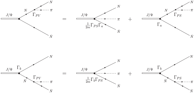
Figure 4:

where the vertices $\Gamma_{a}$, $\Gamma_{b}$, $\Gamma_{PS}$ and $\Gamma_{PV}$ are $\Gamma_{a}=F_{M}\gamma^{\mu}+\frac{1}{2m}F_{0}{(q-p^{\prime})}^{\mu}$, $\Gamma_{b}=F_{M}\gamma^{\mu}+\frac{1}{2m}F_{0}{(p-q^{\prime})}^{\mu}$, $\Gamma_{PS}=ig_{N\bar{N}\pi}\gamma_{5}$ and $\Gamma_{PV}=\frac{i}{2m}g_{N\bar{N}\pi}\gamma_{5}\gamma_{\mu}k^{\mu}$, respectively. The total decay amplitude for Fig. 3 is then obtained by summing over Eq.(8) and Eq.(9)

$${\cal{M}}^{off}_{PV} = {\cal{M}}^{off}_{PV,a}+{\cal{M}}^{off}_{PV,b}$$

$$= \frac{ig_{N\bar{N}\pi}}{2m^{2}}F_{0}\bar{u}(p){(p-p^{\prime})}^{\mu}\epsilon_{\mu}\gamma_{5}v(p^{\prime})+{\cal{M}}_{PS}$$

$$\equiv {\cal{M}}_{PV}.$$

It is clear that in the $J/\psi\to N\bar{N}\pi$ process, when $\pi$-N interaction takes the PS-PV coupling form, the decay amplitude would receive not only the same contribution from PS-PS coupling, but also an extra contribution from contact term. Moreover, the difference of the decay amplitudes in the PS-PS and PS-PV coupling cases only relate to $|F_{0}|$, and are more distinct at the large value of $|F_{0}|$.

The differential decay rate can be formulated by summing over possible spin states of final nucleon and anti-nucleon

$$d\Gamma_{PS}(J/\psi\to N\bar{N}\pi) = \frac{{2\pi}^{4}}{2M_{\psi}}{|{\cal{M}}_{PS}|}^{2}d\Phi_{3}(P_{\psi};p,p^{\prime},k)$$ (12)

$$= {(2\pi)}^{4}\frac{2g^{2}_{N\bar{N}\pi}}{M_{\psi}}~{}[~{}{|F_{M}|}^{2}A_{PS,1}+{|F_{0}|}^{2}A_{PS,2}$$

$$+Re(F^{*}_{0}F_{M})A_{PS,3}~{}]~{}d\Phi_{3}(P_{\psi};p,p^{\prime},k),$$

$$d\Gamma_{PV}(J/\psi\to N\bar{N}\pi) = \frac{{2\pi}^{4}}{2M_{\psi}}{|{\cal{M}}_{PV}|}^{2}d\Phi_{3}(P_{\psi};p,p^{\prime},k)$$ (13)

$$= {(2\pi)}^{4}\frac{2g^{2}_{N\bar{N}\pi}}{M_{\psi}}~{}[~{}{|F_{M}|}^{2}A_{PS,1}+{|F_{0}|}^{2}(A_{PS,2}+A_{PV,2})$$

$$+Re(F^{*}_{0}F_{M})(A_{PS,3}+A_{PV,3})~{}]~{}d\Phi_{3}(P_{\psi};p,p^{\prime},k),$$

with $M_{\psi}$ being the mass of $J/\psi$ and

$$d\Phi_{3}(P_{\psi};p,p^{\prime},k)=\delta^{4}(P_{\psi}-p-p^{\prime}-k)\frac{d^{3}p}{{(2\pi)}^{3}2p_{0}}\frac{d^{3}p^{\prime}}{{(2\pi)}^{3}2p^{\prime}_{0}}\frac{d^{3}k}{{(2\pi)}^{3}2k_{0}}$$ (14)

being an element of three-body phase space. The explicit expressions for $A_{PS,i}(i=1,2,3)$ and $A_{PV,i}(i=2,3)$ are shown in the Appendix. Again, it is found from Eqs.(12) and (13) that the ${|F_{M}|}^{2}$ dependent term does not contribute to the difference between $d\Gamma_{PV}$ and $d\Gamma_{PS}$. If $|F_{0}|=0$, the differential decay rates in the PS-PS and PS-PV coupling cases are absolutely identical.

The value of $|F_{0}|/|F_{M}|$ can be determined in the following way [7]. In the realistic calculation, one usually adopts the electric coupling parameter $F_{E}$ and the magnetic coupling parameter $F_{M}$ instead of $F_{0}$ and $F_{M}$ used above. $F_{0}$ can be expressed by

$$F_{0}=\frac{4m^{2}}{M_{\psi}-4m^{2}}(F_{M}-F_{E}).$$ (15)

Then the squared amplitude for $J/\psi\to p\bar{p}$ decay can be written as

$$\overline{{|{\cal M}|}^{2}}=C_{0}~{}(1+\alpha cos^{2}\theta),$$ (16)

with

$$C_{0}=m^{2}{|F_{M}|}^{2}+4m^{2}{|F_{E}|}^{2},~{}~{}~{}\alpha=[{|F_{M}|}^{2}-\frac{4m^{2}}{M^{2}_{\psi}}{|F_{E}|}^{2}]~{}/~{}[{|F_{M}|}^{2}+\frac{4m^{2}}{M^{2}_{\psi}}{|F_{E}|}^{2}].$$ (17)

By measuring the angular distribution of the $J/\psi\to p\bar{p}$ decay, one obtains $\alpha=0.62\pm 0.11$ [9]. Consequently, $|F_{E}|/|F_{M}|=0.80\pm 0.14$. Assuming

$$\frac{F_{E}}{F_{M}}=\frac{|F_{E}|}{|F_{M}|}~{}e^{i\delta}~{},$$ (18)

one can easily extract the value of $|F_{0}|/|F_{M}|$ by

$$\frac{F_{0}}{F_{M}}=\frac{4m^{2}}{M^{2}_{\psi}-4m^{2}}\left[1-\frac{|F_{E}|}{|F_{M}|}~{}e^{i\delta}\right]~{}.$$ (19)

Taking $\delta=0$, $\frac{\pi}{2}$ and $\pi$, we have

$$\frac{|F_{0}|}{|F_{M}|}=\left\{\begin{array}[]{ll}0.12\pm 0.08&~{}~{}for~{}~{}\delta~{}=0,\\ 0.74\pm 0.08&~{}~{}for~{}~{}\delta~{}={\textstyle\frac{\pi}{2}},\\ 1.04\pm 0.08&~{}~{}for~{}~{}\delta~{}=\pi.\\ \end{array}\right.$$ (20)

The effect of the ratio $|F_{0}|/|F_{M}|$ on $\Gamma_{PS}$ and $\Gamma_{PV}$ can be exhibited by taking $|F_{0}|/|F_{M}|=0,0.12,0.74,1.04$ in our calculation. The branching ratio (BR) of the decay widths for Fig. 3 in the PS-PS and PS-PV cases are

$$\frac{\Gamma_{PS}(J/\psi\to p\bar{p}\pi^{0})}{\Gamma(J/\psi\to p\bar{p})}=\left\{\begin{array}[]{ll}0.556&~{}~{}for~{}|F_{0}|/|F_{M}|~{}=0,\\ 0.561&~{}~{}for~{}|F_{0}|/|F_{M}|~{}=0.12,\\ 0.688&~{}~{}for~{}|F_{0}|/|F_{M}|~{}=0.74,\\ 0.815&~{}~{}for~{}|F_{0}|/|F_{M}|~{}=1.04,\\ \end{array}\right.$$ (21)

and

$$\frac{\Gamma_{PV}(J/\psi\to p\bar{p}\pi^{0})}{\Gamma(J/\psi\to p\bar{p})}=\left\{\begin{array}[]{ll}0.556&~{}~{}for~{}|F_{0}|/|F_{M}|~{}=0,\\ 0.529&~{}~{}for~{}|F_{0}|/|F_{M}|~{}=0.12,\\ 0.475&~{}~{}for~{}|F_{0}|/|F_{M}|~{}=0.74,\\ 0.421&~{}~{}for~{}|F_{0}|/|F_{M}|~{}=1.04,\\ \end{array}\right.$$ (22)

respectively. Comparing with the empirical ratio [8]

$$\frac{\Gamma(J/\psi\to p\bar{p}\pi^{0})}{\Gamma(J/\psi\to p\bar{p})}=0.51\pm 0.04,$$ (23)

one sees that the resultant BRs in Eqs.(21) and (22) are very close to the data. It indicates that the BR of the $J/\psi\to N\bar{N}{\pi}$ decay is dominated by the nucleon-pole diagrams of Fig. 3 without including the hadronic form factor. Of course, the $N^{*}$-pole will also contribute. However, if one would use the data of $J/\psi\to N\bar{N}\pi$ decay to study $N^{*}$, one cannot get meaningful information until the nucleon-pole contribution is considered.

One can also find that the difference due to different $\pi$-N couplings becomes larger when $|F_{0}|/|F_{M}|$ ratio increases. This is because that in the PS-PS coupling case, both the $F_{M}$-dependent term and the $F_{0}$-dependent term contribute positively, but in the PS-PV coupling case, the $F_{M}$-dependent term keeps the same contribution and the $F_{0}$-dependent term gives a negative contribution. Therefore, large $|F_{0}|/|F_{M}|$ value would make the difference larger. For instance, with $|F_{0}|/|F_{M}|=1.04$, the ratio of $\Gamma_{PS}(J/\psi\to p\bar{p}\pi^{0})/\Gamma(J/\psi\to p\bar{p})$ is almost twice of $\Gamma_{PV}(J/\psi\to p\bar{p}\pi^{0})/\Gamma(J/\psi\to p\bar{p})$.

2.2 Off-shell effect with various form factor in the $J/\psi\to N\bar{N}\pi$ decay

Normally, a hadronic form factor is applied to the meson-baryon-baryon ($MBB^{\prime}$) vertices because of the inner quark-gluon structure of hadrons. It is well known that form factor plays an important role in many physics processes, for example, the NN interaction models [10], NN scattering [11], $\pi N$ scattering [12, 13, 14], pion photoproduction [15], vector meson photoproduction [16] and etc.. However, due to the difficulties in dealing with nonperturbative QCD (NPQCD) effects, the form factors are commonly adopted phenomenologically.

The most commonly used form factors for meson-nucleon-nucleon vertices are monopole form factor and dipole form factor [17]:

$$F_{1}(q^{2})=\frac{\Lambda^{2}+m^{2}}{\Lambda^{2}+q^{2}},$$ (24)

$$F_{2}(q^{2})=\frac{\Lambda^{4}+m^{4}}{\Lambda^{4}+q^{4}},$$ (25)

where m and q are the mass and the four-momentum of the intermediate particle, respectively, and $\Lambda$ is the so-called cut-off momentum that can be determined by fitting the experimental data. The monopole form factor is mainly used in the $\pi$-N and N-N interactions, while the dipole one is usually applied to the N-N interaction. The values of $\Lambda$ is different process by process. A typical value of $\Lambda$ for a monopole form factor in the Bonn potential is in the region of 1.3 $\sim$ 2  GeV [10], and for $\pi$-N interaction is about 1.35 GeV. Frankfurt and Strikman [18] analyzed the deep inelastic scattering (DIS) of leptons from nucleons and showed that the DIS data support a $\pi NN$ monopole form factor with $\Lambda\leq 650MeV$.

The exponential form factor is also a frequently used meson-nucleon-nucleon form factor [19],

$$F_{3}(q^{2})=e^{-|q^{2}-m^{2}|/\Lambda^{2}}.$$ (26)

Form factor can also take the following form [20, 21]:

$$F_{4}(q^{2})=\frac{1}{1+{(q^{2}-m^{2})}^{2}/\Lambda^{4}}.$$ (27)

Moreover, in the study of the photoproduction of meson, T.-S. H. Lee et al. [21, 22] chose a form factor with the form of

$$F_{5}({\bf q}^{2})=exp[-({\bf q}^{2}-{\bf q}^{2}_{0})/\Lambda^{2}],$$ (28)

where ${\bf q}$ and ${\bf q}_{0}$ are the three-momentum vectors of the intermediate nucleon at the energy of $\sqrt{s}(s=q^{2})$ and at the nucleon pole position, respectively.

It should be mentioned that all the form factors mentioned above are normalized to unity when the intermediate nucleon is on its mass shell.

To give readers a comprehensive idea of various form factors, we plot them with $\Lambda=0.65$, $1.0$, $1.5$ and $2.0~{}GeV$ in figs.5 and 6,respectively. Fig.5 shows that the $\Lambda$-dependence of the form factors given above. The common feature of these form factors is that their high momentum transfer part is even more reduced when $\Lambda$ value becomes smaller. The momentum-dependent behaviors of these form factors are quite different with different $\Lambda$ values. Fig.6 presents the momentum-dependence of various form factors. The momentum-dependence of form factors $F_{2}$, $F_{3}$ and $F_{4}$ are very sensitive to the $\Lambda$ value, but $F_{1}$’s not. When the value of $\Lambda$ becomes smaller, the difference among various form factors is more pronounced. For instance, when $\Lambda=0.65~{}GeV$, with increase $q^{2}$, $F_{3}$ reduces much more than $F_{1}$ does. Since in the decay processes considered in this paper, the intermediate nucleon is off-shell, introducing an off-shell form factor would suppress the off-shell effect of the nucleon, and the form of the form factor and the value of $\Lambda$ would affect the decay amplitude. Therefore, studying the hadronic vertex form factor can provide a constraint to the data analysis. Moreover, the results of the data fitting can also help us to choose a proper form factor for the $J/\psi\to N\bar{N}M$ investigation.

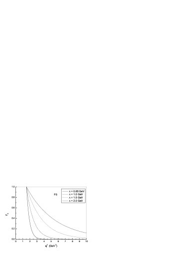
Figure 5: The momentum-dependence of form factors $F_{1}\sim F_{5}$ with different $\Lambda$ values.

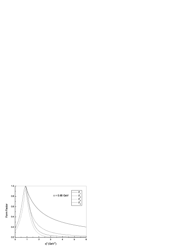
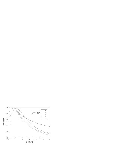
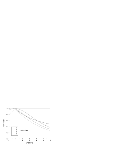
Figure 6: The momentum-dependence of form factors $F_{1}\sim F_{4}$ with the same value of $\Lambda$.

Suppose the form factors with same form are applied on both vertices of the considered decay diagram, respectively. After adding form factors, Eqs. (2.1), (7) and (2.1)can be re-written as

$${\cal{M}}^{\prime}_{PS} = ig_{N\bar{N}\pi}\bar{u}(p)\gamma_{5}~{}\left[~{}F_{M}\left(\frac{/{\hskip-5.69054pt}k~{}/{\hskip-5.69054pt}\epsilon}{2p\cdot k+k^{2}}F^{2}(q^{2})-\frac{/{\hskip-5.69054pt}\epsilon~{}/{\hskip-5.69054pt}k}{2p^{\prime}\cdot k+k^{2}}F^{2}(q^{\prime 2})\right)\right.$$ (29)

$$\left.+\frac{F_{0}}{m}~{}/{\hskip-5.69054pt}k\left(\frac{p\cdot\epsilon}{2p^{\prime}\cdot k+k^{2}}F^{2}(q^{\prime 2})-\frac{p^{\prime}\cdot\epsilon}{2p\cdot k+k^{2}}F^{2}(q^{2})\right)\right]~{}v(p^{\prime}),$$

and

$${\cal{M}}^{\prime}_{PV}=\frac{ig_{N\bar{N}\pi}}{2m}\bar{u}(p)\{F_{M}[F^{2}(q^{2})-F^{2}(q^{\prime 2})]~{}/{\hskip-5.69054pt}\epsilon+\frac{F_{0}}{m}[F^{2}(q^{\prime 2})(p\cdot\epsilon)-F^{2}(q^{2})(p^{\prime}\cdot\epsilon)]\}\gamma_{5}v(p^{\prime})+{\cal{M}}^{\prime}_{PS},$$ (30)

respectively. Form factor $F(q^{2})$ can be chosen to be one of the forms in Eqs. (24) – (28).

In order to show how sensitive the decay BR to the form of the form factor and the value of $\Lambda$, we take $\Lambda=$ 0.65, 1.0, 1.5 and 2.0 GeV and $|F_{0}|/|F_{M}|=0.12\pm 0.08$, and calculate the BR of $\Gamma(J/\psi\to p\bar{p}\pi^{0})/{\Gamma(J/\psi\to p\bar{p})}$ with all kinds of form factors shown above. The results are tabulated in Table 1, where the numbers in parentheses are corresponding to the lower and the upper limits of $|F_{0}|/|F_{M}|$, respectively.

Table 1: The BR of $\Gamma(J/\psi\to p\bar{p}\pi^{0})/\Gamma(J/\psi\to p\bar{p})$ (%) with various form factors.

F.F.	$\pi$N	$\Lambda=0.65~{}GeV$	$\Lambda=1.0~{}GeV$	$\Lambda=1.5~{}GeV$	$\Lambda=2.0~{}GeV$
	coupling
$F_{1}$	PS	3.95(3.73$\sim$4.18)	6.81(6.45$\sim$7.20)	12.69(12.05$\sim$13.38)	19.35(18.40$\sim$20.37)
	PV	2.79(2.77$\sim$2.82)	5.04(5.01$\sim$5.07)	9.96(9.91$\sim$9.98)	15.89(15.83$\sim$15.91)
$F_{2}$	PS	0.34(0.32$\sim$0.37)	1.23(1.15$\sim$1.31)	7.21(6.82$\sim$7.64)	19.64(18.66$\sim$20.71)
	PV	0.20(0.19$\sim$0.21)	0.76(0.75$\sim$0.78)	5.07(5.02$\sim$5.11)	15.50(15.45$\sim$15.53)
$F_{3}$	PS	0.07(0.06$\sim$0.07)	1.09(1.02$\sim$1.16)	5.83(5.51$\sim$6.18)	13.29(12.61$\sim$14.02)
	PV	0.04(0.03 $\sim$ 0.04)	0.66(0.64$\sim$0.68)	4.07(4.03$\sim$4.10)	10.23(10.18$\sim$10.25)
$F_{4}$	PS	0.23(0.22$\sim$0.25)	3.35(3.15$\sim$3.58)	15.03(14.23$\sim$15.89)	29.70(29.68$\sim$31.26)
	PV	0.13(0.12$\sim$0.13)	2.08(2.04$\sim$2.14)	10.98(10.92$\sim$11.04)	24.30(24.23$\sim$24.31)
$F_{5}$	PS	2.39(2.25$\sim$2.54)	10.25(9.71$\sim$10.83)	23.91(22.75$\sim$25.16)	34.01(32.40$\sim$35.72)
	PV	2.33(2.16$\sim$2.81)	9.28(9.37$\sim$9.33)	21.98(22.12$\sim$21.85)	31.57(31.63$\sim$31.44)

From Table 1, one sees that no matter which form factor is employed, the difference between $\Gamma_{PV}(J/\psi\to p\bar{p}\pi^{0})$ and $\Gamma_{PS}(J/\psi\to p\bar{p}\pi^{0})$ is generally larger than that in the without form factor case. For instance, when $\Lambda=1.0~{}GeV$,

$$\frac{\Gamma_{PV}(J/\psi\to p\bar{p}\pi^{0})}{\Gamma_{PS}(J/\psi\to p\bar{p}\pi^{0})}=\left\{\begin{array}[]{ll}0.74&~{}~{}for~{}~{}F_{1}~{},\\ 0.618&~{}~{}for~{}~{}F_{2}~{},\\ 0.606&~{}~{}for~{}~{}F_{3}~{},\\ 0.621&~{}~{}for~{}~{}F_{4}~{},\\ 0.905&~{}~{}for~{}~{}F_{5}~{},\\ \end{array}\right.$$ (31)

and the corresponding ratio without form factors is

$$\frac{\Gamma_{PV}(J/\psi\to p\bar{p}\pi^{0})}{\Gamma_{PS}(J/\psi\to p\bar{p}\pi^{0})}\simeq 0.940~{}.$$ (32)

It means that introduced form factor suppresses the contribution at the large momentum transfer region, and consequently, enlarges the off-shell effects in the PS-PS and PS-PV coupling cases in different extent. For a specific form factor, when the $\Lambda$ value reduces, the curve of the form factor bends towards the lower momentum direction. It further suppresses the contribution at the high momentum transfer region, enlarges the off-shell effect and reduces the nucleon-pole contribution. For instance, with form factor $F_{5}$, when $\Lambda$ reduces from 2.0 GeV to 0.65 GeV, BR $\frac{\Gamma_{PV}(J/\psi\to p\bar{p}\pi^{0})}{\Gamma(J/\psi\to p\bar{p})}$ declines from 31.57% to 2.33%. The $\Lambda$ dependence of the BR differs in different form factor cases. For the same amount of $\Lambda$ value change, BR with $F_{1}$ decreases about 1/5, but BR with $F_{3}$ drops about 1/256. The BR with a larger $\Lambda$ value is more pronounced, and the nucleon-pole contribution is important. On the contrary, the nucleon-pole contribution by using a small $\Lambda$ value can be ignored.

The BR with different form factor but the same $\Lambda$ value is quite different. For example, when $\Lambda=0.65~{}GeV$, the BR with $F_{3}$ and $F_{1}$ in the PS-PV coupling case are about 0.04% and 2.79%, respectively. The later is about 70 times larger than the former one. Anyway, these BRs are negligibly compared with the data of 51%. However, when $\Lambda$ is large, the difference between different form factor cases becomes very small, consequently, the contribution from the high momentum part is not much suppressed, the resultant BRs in both PS-PS and PS-PV cases are close to each other and are comparable with the data. For instance, when $\Lambda=2.0~{}GeV$, the maximum range of BR change is from 10.23% to 34.01%.

Since it is not sure which form factor is suitable for considered decay processes, we cannot conclude whether the nucleon-pole is dominantly responsible for the BR of $J/\psi\to N\bar{N}\pi$ decay. Now, we would show how much the nucleon-pole diagram would contribute to the BR of $J/\psi\to N\bar{N}\pi$, when a form factor used in a similar processes is adopted. It should be mentioned that although all the form factors shown above are the $NN\pi$ vertex form factor, the particle that the momentum variable corresponds to is different case by case. In the N-N interaction, the form factor is $\pi$-momentum dependent, and in the $\pi$-N interaction, the pion photoproduction, and the $J/\psi\to N\bar{N}\pi$ decay, it is intermediate-nucleon-momentum dependent. Only in the case that the form factor depends on the four-momenta of three interacting particles [12], a unified form factor with the same proper parameter $\Lambda$ can possibly be applied to all mentioned processes. We summarize part of form factors whose momentum dependence is similar to the $J/\psi\to N\bar{N}\pi$ decay and whose $\Lambda$ value has well been determined by the $\pi$-N scattering or the pion photoproduction in Table 2.

Table 2: Frequently used $\pi NN$ form factor in literatures.

$\pi N$ Coupling	Coupling Constant	F.F.	$\Lambda$(cut-off)	Ref.
PV	$f^{2}_{\pi NN}/4\pi=0.0778$	$F_{1}(q^{2})$	$1350~{}MeV$	[14]
PV	$g^{2}_{\pi NN}/4\pi=14.3$	$F_{4}(q^{2})$	$1116.6~{}MeV$	[13]
PV	$f^{2}_{\pi NN}/4\pi=0.0778$	$F_{4}(q^{2})$	$1200~{}MeV$	[14]
PS	$g^{2}_{\pi NN}/4\pi=14$	$F_{5}(q^{2})$	$1000~{}MeV$	[21]

With these form factors, we re-calculate the BR of $\Gamma(J/\psi\to p\bar{p}\pi^{0})/\Gamma(J/\psi\to p\bar{p})$. The resultant BRs with $|F_{0}|/|F_{M}|=0.12$ are:

$$\frac{\Gamma(J/\psi\to p\bar{p}\pi^{0})}{\Gamma(J/\psi\to p\bar{p})}=\left\{\begin{array}[]{ll}0.0808&~{}~{}for~{}~{}F_{1}~{},\\ 0.0465&~{}~{}for~{}~{}F_{4}~{},\\ 0.0967&~{}~{}for~{}~{}F_{5}~{}.\\ \end{array}\right.$$ (33)

And those with $|F_{0}|/|F_{M}|=1.04$ are:

$$\frac{\Gamma(J/\psi\to p\bar{p}\pi^{0})}{\Gamma(J/\psi\to p\bar{p})}=\left\{\begin{array}[]{ll}0.0735&~{}~{}for~{}~{}F_{1}~{},\\ 0.0524&~{}~{}for~{}~{}F_{4}~{},\\ 0.1636&~{}~{}for~{}~{}F_{5}~{}.\\ \end{array}\right.$$ (34)

Comparing with the results in Table 1, one finds that the resultant BRs do not differ as much large as those in Table 1, but there is still visible difference.

Although the magnitude of BR is much smaller than data, it can still be used to select a proper form factor for the $J/\psi\to N\bar{N}\pi$ decay. To fulfil this goal, in terms of the Monte Carlo simulation, we calculate the Dalitz plot and the invariant $p\pi^{0}$ mass distribution of the $J/\psi\to p\bar{p}\pi^{0}$ decay with the form factors $F_{1}$, $F_{4}$, and $F_{5}$, respectively. They are shown in Fig. 7.

Figure 7: The Dalitz plot and the invariant $p\pi^{0}$ mass distribution of the $J/\psi\to p\bar{p}\pi^{0}$ decay with the form factors $F_{1}$, $F_{4}$, and $F_{5}$. The solid curve, the dotted-dashed curve and the stared curve in the invariant mass distribution figure correspond to the form factors $F_{1}$, $F_{4}$, and $F_{5}$, respectively.

Comparing these figures with the data, one should be able to find out a most suitable form factor for the $J/\psi\to p\bar{p}\pi^{0}$ decay.

2.3 Nucleon-pole contributions in $J/\psi\to p\bar{p}\eta$ and $J/\psi\to p\bar{p}\eta^{\prime}$ decays

Figure 8: Proton-pole diagrams for $J/\psi\to p\bar{p}\eta$ and $J/\psi\to p\bar{p}\eta^{\prime}$ decays.

The corresponding Feynman diagrams for $J/\psi\to p\bar{p}\eta$ and $p\bar{p}\eta^{\prime}$ decays are shown in Fig. 8. The same formulae for $J/\psi\to p\bar{p}\pi^{0}$ decay can be applied to the $J/\psi\to p\bar{p}\eta$ and $J/\psi\to p\bar{p}\eta^{\prime}$ decays, except replacing $g_{N\bar{N}\pi}$ with $g_{N\bar{N}\eta}$ or $g_{N\bar{N}\eta^{\prime}}$, because $\pi$, $\eta$ and $\eta^{\prime}$ are all pseudoscalar mesons. The values of $g_{N\bar{N}\eta}$ and $g_{N\bar{N}\eta^{\prime}}$ can be chosen according to following relations [7]:

$${(g_{\eta NN}/g_{\pi NN})}^{2}=3.90625\times 10^{-3},~{}~{}~{}~{}{(g_{\eta^{\prime}NN}/g_{\pi NN})}^{2}=2.5\times 10^{-3}~{}.$$ (35)

And we take $|F_{0}|/|F_{M}|=0,0.12,0.74$ and $1.04$ in our calculation. The decay ratios of $\Gamma(J/\psi\to p\bar{p}\eta)/\Gamma(J/\psi\to p\bar{p})$ and $\Gamma(J/\psi\to p\bar{p}\eta^{\prime})/\Gamma(J/\psi\to p\bar{p})$ from the proton-pole contribution without considering form factors are:

$$\frac{\Gamma_{PS}(J/\psi\to p\bar{p}\eta)}{\Gamma(J/\psi\to p\bar{p})}=\left\{\begin{array}[]{ll}5.48\times 10^{-4}&~{}~{}for~{}|F_{0}|/|F_{M}|~{}=0~{},\\ 5.63\times 10^{-4}&~{}~{}for~{}|F_{0}|/|F_{M}|~{}=0.12~{},\\ 6.91\times 10^{-4}&~{}~{}for~{}|F_{0}|/|F_{M}|~{}=0.74~{},\\ 8.19\times 10^{-4}&~{}~{}for~{}|F_{0}|/|F_{M}|~{}=1.04~{},\\ \end{array}\right.$$ (36)

$$\frac{\Gamma_{PV}(J/\psi\to p\bar{p}\eta)}{\Gamma(J/\psi\to p\bar{p})}=\left\{\begin{array}[]{ll}5.48\times 10^{-4}&~{}~{}for~{}|F_{0}|/|F_{M}|~{}=0~{},\\ 5.26\times 10^{-4}&~{}~{}for~{}|F_{0}|/|F_{M}|~{}=0.12~{},\\ 4.69\times 10^{-4}&~{}~{}for~{}|F_{0}|/|F_{M}|~{}=0.74~{},\\ 4.12\times 10^{-4}&~{}~{}for~{}|F_{0}|/|F_{M}|~{}=1.04~{},\\ \end{array}\right.$$ (37)

and

$$\frac{\Gamma_{PS}(J/\psi\to p\bar{p}\eta^{\prime})}{\Gamma(J/\psi\to p\bar{p})}=\left\{\begin{array}[]{ll}1.93\times 10^{-5}&~{}~{}for~{}|F_{0}|/|F_{M}|~{}=0~{},\\ 1.99\times 10^{-5}&~{}~{}for~{}|F_{0}|/|F_{M}|~{}=0.12~{},\\ 2.45\times 10^{-5}&~{}~{}for~{}|F_{0}|/|F_{M}|~{}=0.74~{},\\ 2.91\times 10^{-5}&~{}~{}for~{}|F_{0}|/|F_{M}|~{}=1.04~{},\\ \end{array}\right.$$ (38)

$$\frac{\Gamma_{PV}(J/\psi\to p\bar{p}\eta^{\prime})}{\Gamma(J/\psi\to p\bar{p})}=\left\{\begin{array}[]{ll}1.93\times 10^{-5}&~{}~{}for~{}|F_{0}|/|F_{M}|~{}=0~{},\\ 1.87\times 10^{-5}&~{}~{}for~{}|F_{0}|/|F_{M}|~{}=0.12~{},\\ 1.70\times 10^{-5}&~{}~{}for~{}|F_{0}|/|F_{M}|~{}=0.74~{},\\ 1.54\times 10^{-5}&~{}~{}for~{}|F_{0}|/|F_{M}|~{}=1.04~{}.\\ \end{array}\right.$$ (39)

Again, the difference of BRs between PS-PS and PS-PV couplings descents when the ratio of $|F_{0}|/|F_{M}|$ declines. Comparing with the empirical data of $\Gamma(J/\psi\to p\bar{p}\eta)/\Gamma(J/\psi\to p\bar{p})=0.98\pm 0.09$ and $\Gamma(J/\psi\to p\bar{p}\eta^{\prime})/\Gamma(J/\psi\to p\bar{p})=0.42\pm 0.19$ [8], one finds that the calculated BRs are all smaller than 0.1% of the data. This is because that in these two decays, the intermediate nucleon is largely off-shell. We also tabulate the BRs of $\frac{\Gamma(J/\psi\to p\bar{p}\eta)}{\Gamma(J/\psi\to p\bar{p})}$ and $\frac{\Gamma(J/\psi\to p\bar{p}\eta^{\prime})}{\Gamma(J/\psi\to p\bar{p})}$ with various $\pi NN$ form factors in Tables 3 and 4, respectively. Because the form factor further reduces the proton-pole contribution at the high momentum region, the resultant BRs are very small. Therefore, in analyzing the $J/\psi\to p\bar{p}\eta$ and $J/\psi\to p\bar{p}\eta^{\prime}$ data, the proton-pole contribution can safely be ignored. The main contributor for such decays must be some other diagrams, for instance, the $N^{*}$-pole diagram.

Table 3: Branching ratio $\Gamma(J/\psi\to p\bar{p}\eta)/{\Gamma(J/\psi\to p\bar{p})}$ with form factors, with $|F_{0}|/|F_{M}|=0.12.$

F.F.	$\pi\eta$	$\Lambda=0.65GeV$	$\Lambda=1.0GeV$	$\Lambda=1.5GeV$	$\Lambda=2.0GeV$
	coupling
$F_{1}$	PS	$9.61\times 10^{-6}$	$2.24\times 10^{-5}$	$5.92\times 10^{-5}$	$1.14\times 10^{-4}$
	PV	$7.26\times 10^{-6}$	$1.74\times 10^{-5}$	$4.77\times 10^{-5}$	$9.49\times 10^{-5}$
$F_{2}$	PS	$6.34\times 10^{-8}$	$5.04\times 10^{-7}$	$1.31\times 10^{-5}$	$8.90\times 10^{-5}$
	PV	$4.15\times 10^{-8}$	$3.35\times 10^{-7}$	$9.26\times 10^{-6}$	$6.91\times 10^{-5}$
$F_{3}$	PS	$2.63\times 10^{-11}$	$1.54\times 10^{-7}$	$1.00\times 10^{-5}$	$5.31\times 10^{-5}$
	PV	$1.63\times 10^{-11}$	$1.01\times 10^{-7}$	$7.02\times 10^{-6}$	$4.09\times 10^{-5}$
$F_{4}$	PS	$1.77\times 10^{-9}$	$6.77\times 10^{-7}$	$3.40\times 10^{-5}$	$1.63\times 10^{-4}$
	PV	$1.11\times 10^{-9}$	$4.37\times 10^{-7}$	$2.39\times 10^{-5}$	$1.29\times 10^{-4}$
$F_{5}$	PS	$7.06\times 10^{-7}$	$2.64\times 10^{-5}$	$1.38\times 10^{-4}$	$2.52\times 10^{-4}$
	PV	$3.66\times 10^{-6}$	$2.19\times 10^{-5}$	$1.22\times 10^{-4}$	$2.29\times 10^{-4}$

Table 4: Branching ratio $\Gamma(J/\psi\to p\bar{p}\eta^{\prime})/{\Gamma(J/\psi\to p\bar{p})}$ with form factors, with $|F_{0}|/|F_{M}|=0.12.$

F.F.	$\pi\eta^{\prime}$	$\Lambda=0.65GeV$	$\Lambda=1.0GeV$	$\Lambda=1.5GeV$	$\Lambda=2.0GeV$
	coupling
$F_{1}$	PS	$1.35\times 10^{-7}$	$3.61\times 10^{-7}$	$1.16\times 10^{-6}$	$2.59\times 10^{-6}$
	PV	$1.14\times 10^{-7}$	$3.09\times 10^{-7}$	$1.01\times 10^{-6}$	$2.28\times 10^{-6}$
$F_{2}$	PS	$1.99\times 10^{-10}$	$1.96\times 10^{-9}$	$9.94\times 10^{-8}$	$1.33\times 10^{-6}$
	PV	$1.53\times 10^{-10}$	$1.52\times 10^{-9}$	$7.93\times 10^{-8}$	$1.11\times 10^{-6}$
$F_{3}$	PS	$4.78\times 10^{-18}$	$5.99\times 10^{-11}$	$6.40\times 10^{-8}$	$7.76\times 10^{-7}$
	PV	$3.62\times 10^{-18}$	$4.16\times 10^{-11}$	$4.99\times 10^{-8}$	$6.50\times 10^{-7}$
$F_{4}$	PS	$1.70\times 10^{-12}$	$1.22\times 10^{-9}$	$2.28\times 10^{-7}$	$2.63\times 10^{-6}$
	PV	$1.26\times 10^{-12}$	$9.15\times 10^{-10}$	$1.79\times 10^{-7}$	$2.21\times 10^{-6}$
$F_{5}$	PS	$8.13\times 10^{-10}$	$2.67\times 10^{-7}$	$2.91\times 10^{-6}$	$6.75\times 10^{-6}$
	PV	$1.23\times 10^{-7}$	$2.32\times 10^{-7}$	$2.50\times 10^{-6}$	$6.05\times 10^{-6}$

3 Nucleon-pole contribution in the $J/\psi\to p\bar{p}\omega$ decay

The nucleon-pole diagram in the $J/\psi\to p\bar{p}\omega$ decay are shown in Fig.9,

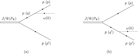
Figure 9: Proton-pole diagram for $J/\psi\to p\bar{p}\omega$ decay.

where the variables in brackets are four-momenta of corresponding particles. The mass of $\omega$ meson is 781.94MeV. Due to heavy mass of $\omega$, the intermediate nucleon in Fig.9 must be far from the mass shell.

The $NN\omega$ interaction can be written as [7]

$$H_{\omega NN}=g_{\omega NN}\bar{N}(x)\gamma^{\alpha}N(x)\omega_{\alpha}(x)+i\frac{1}{4m}f_{\omega NN}\bar{N}(x)[\gamma^{\mu},\gamma^{\nu}]N(x)\partial_{\mu}\omega_{\nu}(x)~{}.$$ (40)

The vector coupling constant $g_{\omega NN}$ and tensor coupling constant $f_{\omega NN}$ are:

$$g_{\omega pp}^{2}/4\pi\simeq 6.3~{},$$ (41)

$$f_{\omega pp}=(\mu_{p}+\mu_{n})g_{\omega pp}~{},$$ (42)

respectively, with the anomalous magnetic moments of proton and neutron

$$\mu_{p}=1.7928\mu_{N}~{},~{}~{}~{}~{}~{}~{}~{}\mu_{n}=-1.9131\mu_{N}~{},$$ (43)

respectively. A simple manipulation gives

$$f_{\omega pp}\simeq-0.12g_{\omega pp}~{}.$$ (44)

Therefore, the $\omega NN$ interaction is mainly vector coupling.

Similar to what Y. Oh and T-S.H. Lee did [15, 23] in the vector meson photoproduction study, we only take the vector coupling in the $J/\psi\to p\bar{p}\omega$ calculation

$$H_{\omega NN}^{\prime}=g_{\omega NN}\bar{N}(x)\gamma^{\alpha}N(x)\omega_{\alpha}(x)~{}.$$ (45)

Performing similar derivation in the $J/\psi\to p\bar{p}\pi^{0}$ case and using the properties

$$P_{\psi}^{\beta}\epsilon_{\beta}(P_{\psi},\lambda)=0~{},~{}~{}~{}~{}k^{\alpha}e_{\alpha}(k,\lambda^{\prime})=0~{},$$ (46)

where $\epsilon_{\beta}(P_{\psi},\lambda)$ and $e_{\alpha}(k,\lambda^{\prime})$ are polarization vectors of $J/\psi$ and $\omega$, respectively, we get the total decay amplitude for Fig. 9

$${\cal M} = g_{\omega pp}~{}\bar{u}(p,s)\left\{F_{M}\left[~{}\frac{2p\cdot e+/{\hskip-5.69054pt}e/{\hskip-5.69054pt}k}{2p\cdot k+k^{2}}~{}/{\hskip-5.69054pt}\epsilon-/{\hskip-5.69054pt}\epsilon~{}\frac{2p^{\prime}\cdot e+/{\hskip-5.69054pt}k/{\hskip-5.69054pt}e}{2p^{\prime}\cdot k+k^{2}}~{}\right]\right.$$ (47)

$$-\frac{F_{0}}{m}\left.\left[~{}(p^{\prime}\cdot\epsilon)~{}\frac{2p\cdot e+/{\hskip-5.69054pt}e/{\hskip-5.69054pt}k}{2p\cdot k+k^{2}}+(p\cdot\epsilon)~{}\frac{2p^{\prime}\cdot e+/{\hskip-5.69054pt}k/{\hskip-5.69054pt}e}{2p^{\prime}\cdot k+k^{2}}~{}\right]\right\}v(p^{\prime},s^{\prime})~{},$$

and the differential decay width by summing over possible spin states of the initiate and final particles

$$d\Gamma(J/\psi\to p\bar{p}\omega)=\frac{2\pi^{4}}{2M_{\psi}}~{}\overline{\left|{\cal M}\right|^{2}}~{}d\Phi_{3}(P_{\psi};p,p^{\prime},k)~{}.$$ (48)

Taking $|F_{0}|/|F_{M}|=0$, $0.12$, $0.74$ and $1.04$, we obtain the branching ratio

$$\frac{\Gamma(J/\psi\to p\bar{p}\omega)}{\Gamma(J/\psi\to p\bar{p})}=\left\{\begin{array}[]{ll}0.169&~{}~{}for~{}|F_{0}|/|F_{M}|~{}=0~{},\\ 0.168&~{}~{}for~{}|F_{0}|/|F_{M}|~{}=0.12~{},\\ 0.171&~{}~{}for~{}|F_{0}|/|F_{M}|~{}=0.74~{},\\ 0.175&~{}~{}for~{}|F_{0}|/|F_{M}|~{}=1.04~{}.\\ \end{array}\right.$$ (49)

In comparison with the data of $0.61\pm 0.12$ [8] one sees that without considering form factor, the proton-pole diagram provides rather important contribution to the width of the $J/\psi\to p\bar{p}\omega$ decay. As mentioned above, because $\omega$ is relative heavy, the intermediate proton should be far from mass shell, the terms with high power of momentum in the amplitude make the amplitude vs momentum curve bent upward and gone apart from the normal Breit-Wigner form. This non-physical feature of the amplitude at the high momentum region should be suppressed by adding off-shell form factors.

After including the form factor, the decay amplitude becomes

$${\cal M}^{\prime} = g_{\omega pp}~{}\bar{u}(p,s)\left\{F_{M}\left[~{}\frac{2p\cdot e+/{\hskip-5.69054pt}e/{\hskip-5.69054pt}k}{2p\cdot k+k^{2}}~{}F^{2}(q^{2})~{}/{\hskip-5.69054pt}\epsilon-/{\hskip-5.69054pt}\epsilon~{}\frac{2p^{\prime}\cdot e+/{\hskip-5.69054pt}k/{\hskip-5.69054pt}e}{2p^{\prime}\cdot k+k^{2}}~{}F^{2}(q^{\prime 2})~{}\right]\right.$$ (50)

$$~{}~{}~{}~{}~{}~{}~{}~{}~{}~{}~{}~{}~{}~{}~{}~{}~{}~{}~{}~{}-\frac{F_{0}}{m}\left[~{}(p^{\prime}\cdot\epsilon)~{}\frac{2p\cdot e+/{\hskip-5.69054pt}e/{\hskip-5.69054pt}k}{2p\cdot k+k^{2}}~{}F^{2}(q^{2})\right.$$

$$\left.\left.~{}~{}~{}~{}~{}~{}~{}~{}~{}~{}~{}~{}~{}~{}~{}~{}~{}~{}~{}~{}~{}~{}~{}~{}~{}~{}~{}~{}~{}~{}~{}+(p\cdot\epsilon)~{}\frac{2p^{\prime}\cdot e+/{\hskip-5.69054pt}k/{\hskip-5.69054pt}e}{2p^{\prime}\cdot k+k^{2}}~{}F^{2}(q^{\prime 2})~{}\right]\right\}v(p^{\prime},s^{\prime})~{},$$

where the form factor $F(q^{2})$ can be any one from Eqs. (24)-(28). Taking $|F_{0}|/|F_{M}|=0.12$ again, we obtain the BRs of $\Gamma(J/\psi\to p\bar{p}\omega)/\Gamma(J/\psi\to p\bar{p})$. They are tabulated in Table 5.

Table 5: The branching ratio of $\Gamma(J/\psi\to p\bar{p}\omega)/{\Gamma(J/\psi\to p\bar{p})}$ decay with form factor.

F.F.	$\Lambda=0.65~{}GeV$	$\Lambda=1.0~{}GeV$	$\Lambda=1.5~{}GeV$	$\Lambda=2.0~{}GeV$
$F_{1}$	1.48$\times 10^{-3}$	3.83$\times 10^{-3}$	1.16$\times 10^{-2}$	2.49$\times 10^{-2}$
$F_{2}$	3.34$\times 10^{-6}$	3.15$\times 10^{-5}$	1.35$\times 10^{-3}$	1.48$\times 10^{-2}$
$F_{3}$	5.03$\times 10^{-12}$	2.45$\times 10^{-6}$	9.40$\times 10^{-4}$	8.66$\times 10^{-3}$
$F_{4}$	3.83$\times 10^{-8}$	2.43$\times 10^{-5}$	3.27$\times 10^{-3}$	2.88$\times 10^{-2}$
$F_{5}$	2.02$\times 10^{-5}$	3.28$\times 10^{-3}$	2.86$\times 10^{-2}$	6.18$\times 10^{-2}$

From this table, one finds that the proton-pole contribution is sensitive to the form of the form factor and the value of $\Lambda$. The most $\Lambda$-sensitive form factor is $F_{3}$, with which BR changes to almost $10^{8}$ times as much when $\Lambda$ increases from 0.65 GeV to 2.0 GeV. The most $\Lambda$-insensitive one is $F_{1}$, with which BR only increases to 17 times as much. Moreover, when $\Lambda$ is small, the BR is more sensitive to the form of the form factor. For instance, with $\Lambda=0.65~{}GeV$, the resultant BRs from various form factors have almost $10^{9}$ times difference. But with $\Lambda=2.0~{}GeV$, the difference is just about 3 times. The reason is the same as that in the $J/\psi\to p\bar{p}\pi^{0}$ case. We also provide the relevant Dalitz plot and the invariant mass distribution of $p\omega$. The Dalitz plot in these figures shows that the contributions of the proton-pole diagram at the high momentum region is evidently suppressed. This agrees with our conjecture mentioned at the beginning of this section.

Figure 10: The Dalitz plot and the $p\omega$ invariant mass distribution in $J/\psi\to p\bar{p}\omega$ decay ( $\Lambda=0.65~{}GeV$ ). The solid, dashed, dotted, dotted-dashed and stared curves denote the cases with $F_{1}$, $F_{2}$, $F_{3}$, $F_{4}$ and $F_{5}$, respectively

Figure 11: The Dalitz plot and the $p\omega$ invariant mass distribution in $J/\psi\to p\bar{p}\omega$ decay ( $\Lambda=1.0~{}GeV$ ). The solid, dashed, dotted, dotted-dashed and stared curves denote the cases with $F_{1}$, $F_{2}$, $F_{3}$, $F_{4}$ and $F_{5}$, respectively

Figure 12: The Dalitz plot and the $p\omega$ invariant mass distribution in $J/\psi\to p\bar{p}\omega$ decay ( $\Lambda=1.5~{}GeV$ ). The solid, dashed, dotted, dotted-dashed and stared curves denote the cases with $F_{1}$, $F_{2}$, $F_{3}$, $F_{4}$ and $F_{5}$, respectively

Figure 13: The Dalitz plot and the $p\omega$ invariant mass distribution in $J/\psi\to p\bar{p}\omega$ decay ( $\Lambda=2.0~{}GeV$ ). The solid, dashed, dotted, dotted-dashed and stared curves denote the cases with $F_{1}$, $F_{2}$, $F_{3}$, $F_{4}$ and $F_{5}$, respectively

Furthermore, comparing with the data of $0.61\pm 0.12$

in PDG [8], we find that the resultant BRs are generally less than 10% of the data. This indicates that in the $J/\psi\to p\bar{p}\omega$ decay, the proton-pole contribution is not so important. To explain the empirical data, there must be certain contributions from other diagrams such as the $N^{*}$-pole diagram.

4 conclusion

$J/\psi\to N\bar{N}M$ decay is an ideal process to study $N^{*}$ spectrum. As intermediate states, nucleon and $N^{*}$ can all contribute to the decay BR. In the $J/\psi\to N\bar{N}M$ decay data analysis, nucleon-pole contribution would play an important role of background. Understanding this contribution would enable us to get a more accurate and more reliable information of $N^{*}$. In this paper, we study the nucleon-pole contribution by employing PS-PS and PS-PV $\pi N\bar{N}$ vertex couplings and various vertex form factors.

According to the equivalent theorem [24], the PS-PS and PS-PV couplings of $\pi$-N interaction are equivalent, when the intermediate nucleon is on-shell. Namely, the decay amplitudes with the PS-PS and PS-PV coupling vertices are exactly the same. But, when the intermediate nucleon is off-shell, their decay amplitudes are different. The amplitude with the PS-PS coupling vertex keeps the same form as in the on-shell case, and the amplitude with the PS-PV coupling vertex has an additional term which describes a four particle contact interaction. It seems that the PS-PV coupling contains PS-PS coupling. In fact, many authors claimed that using PS-PV coupling only is good enough in describing the $\pi$-N interaction and the meson photoproduction [13, 14, 15, 25, 26]. But some authors believed that a mixed coupling

$$g_{\pi NN}\tau_{i}\left[\lambda\gamma_{5}-(1-\lambda)\frac{/{\hskip-5.69054pt}p-/{\hskip-5.69054pt}p^{\prime}}{2m}\gamma_{5}\right]~{},$$ (51)

where $\lambda$ is a mixing parameter, is more appropriate [11, 12, 27]. The value of $\lambda$ can be extracted by data fitting. For an example, Gross, Orden and Holinde [11] obtained $\lambda\cong 0.22$ by fitting the N-N data in a one-boson exchange (OBE) model, Goudsmit Leisi and Mastinos found $\lambda\cong 0.24$ by analyzing the $\pi$-N scattering data at the tree diagram level [27], Gross and Surya got $\lambda\cong 0.25$ by fitting the $\pi$-N scattering data [12]. Anyway, the obtained $\lambda$ value shows that in the mixed $NN\pi$ vetex, PS-PS coupling only occupies a samll portion.

Because PS-PS and PS-PV couplings are not equivalent when the intermediate nucleon is off-shell, the resultant nucleon-pole contribution to $\Gamma(J/\psi\to p\bar{p}\pi^{0})/\Gamma(J/\psi\to p\bar{p})$ in these cases are different. The smaller the $|F_{0}|/|F_{M}|$ ratio in the $J/\psi\to p\bar{p}$ decay is, the closer the BRs in the PS-PS and PS-PV cases are. For instance, when $|F_{0}|/|F_{M}|=0.12$, the mentioned difference is quite small, and the ratio $\Gamma_{PV}(J/\psi\to p\bar{p}\pi^{0})/\Gamma_{PS}(J/\psi\to p\bar{p}\pi^{0})$ is about 0.94. The resultant BR is about 0.53. In comparison with the data of 0.51, one can claim that the proton-pole diagram is the main contributor to be responsible for the BR of the $J/\psi\to p\bar{p}\pi^{0}$ decay.

On the other hand, hadron has its own inner structure. To be realistic, one has to introduce vertex form factors. After considering the form factor, the mentioned BR difference is enlarged. The size of the change depends on the form of the form factor and its $\Lambda$ value. In general, the smaller the $\Lambda$ is, the large the difference would be. When $\Lambda$ is small, say $\Lambda=0.65~{}GeV$, the resultant BR of $J/\psi\to p\bar{p}\pi^{0}$ depends strongly on the form of the form factor. When the form factor takes an exponential form or a dipole form, it highly suppresses the contribution at the high momentum part, and consequently, the resultant BR reduces to 0.08% or 0.4% of the value obtained without form factor. When $\Lambda$ is large, say $\Lambda=2.0~{}GeV$, all the form factors become very similar to each other, the form factor curves do not declined too much, and then the resultant BRs are also very similar and are not small. They are about 20% to 30% of the value without form factor.

The $\Lambda$-sensitivity of various form factors are also different. The exponential form factor is the most sensitive one. When $\Lambda$ value changes from 0.65 GeV to 2.0 GeV, the BR changes about 256 times as much. But for a most-insensitive one (monopole form factor), the change is only about 6 times as much.

Moreover, if one adopts a form factor that are frequently used in explaining the $\pi$-N scattering and the pion photoproduction data, the proton-pole contribution is about $10\sim 20$% of the $J/\psi\to p\bar{p}\pi^{0}$ data. Thus, the proton-pole diagram must be accounted.

The similar results for the $J/\psi\to p\bar{p}\eta$ and $p\bar{p}\eta^{\prime}$ are studied in the same manner. Taking $|F_{0}|/|F_{M}|=0.12$ and without considering the form factor, the resultant BRs from the proton-pole diagram are $5\times 10^{-4}$ and $2\times 10^{-4}$, for the $J/\psi\to p\bar{p}\eta$ and $p\bar{p}\eta^{\prime}$ decays, respectively. In comparison with the data of $0.98$ and $0.42$, they are all less than $0.1$% of the data. Taking the form factor into account, the resultant BRs are further reduced. Therefore, in analyzing the $J/\psi\to p\bar{p}\eta$ and $p\bar{p}\eta^{\prime}$ decay data, the contribution from the proton-pole diagram can safely be ignored.

The proton-pole diagram contribution to the $J/\psi\to p\bar{p}\omega$ decay is analyzed too. The difference between resultant BRs by using vector coupling and mixed coupling is only about 3%. Comparing with the data of 0.61, without considering the form factor and with $|F_{0}|/|F_{M}|=0.12$, the BR obtained from the proton-pole diagram is about 0.168, which is about 28% of the data. When the form factor is considered, the obtained largest BR is less than 10% of the data. This indicates that other diagram such as $N^{*}$-pole diagram may be mainly responsible for the $J/\psi\to p\bar{p}\omega$ decay.

Finally, it is worthy to know that through $J/\psi$ decay data fitting, it is possible to select an appropriate form factor for the $J/\psi\to N\bar{N}M$ decay.

ACKNOWLEDGMENTS

The authors would like to thank Professor Rahul Sinha for his fruitful discussion. We also thank Wei-Xing Ma for useful discussions. This work is partly supported by National Science Foundation of China under contract Nos. 10075057, 90103020, 19991487, 10225525 and 10147202, the CAS Knowledge Innovation Key Project KJCX2-SW-N02, and the Deutsche Forschungsgemeinschaft.

APPENDIX

In this appendix, we give the explicit expressions of $A_{PS,i}(i=1,2,3)$ and $A_{PV,i}(i=2,3)$ appeared in Eqs.(12) and (13),

$$A_{PS,1} = (m^{2}+p\cdot p^{\prime})~{}[~{}(a^{2}-b^{2}){(\epsilon\cdot k)}^{2}+b^{2}\epsilon^{2}k^{2}~{}]$$ (52)

$$-2ab(\epsilon\cdot k)~{}[~{}(\epsilon\cdot p)(p^{\prime}\cdot k)-(\epsilon\cdot p^{\prime})(p\cdot k)~{}]$$

$$-2b^{2}~{}[~{}\epsilon^{2}(p\cdot k)(p^{\prime}\cdot k)-(\epsilon\cdot k)(\epsilon\cdot p^{\prime})(p\cdot k)-(\epsilon\cdot k)(\epsilon\cdot p)(p^{\prime}\cdot k)$$

$$+k^{2}(\epsilon\cdot p)(\epsilon\cdot p^{\prime})~{}]~{},$$

$$A_{PS,2}=\frac{1}{m^{2}}~{}[~{}(m^{2}-p\cdot p^{\prime})k^{2}+2(p\cdot k)(p^{\prime}\cdot k)~{}]{\left[\frac{p^{\prime}\cdot\epsilon}{2p\cdot k+k^{2}}-\frac{p\cdot\epsilon}{2p^{\prime}\cdot k+k^{2}}\right]}^{2},$$ (53)

$$A_{PS,3}=4k^{2}{\left[\frac{p^{\prime}\cdot\epsilon}{2p\cdot k+k^{2}}-\frac{p\cdot\epsilon}{2p^{\prime}\cdot k+k^{2}}\right]}^{2}~{},$$ (54)

$$A_{PV,2} = \frac{1}{m^{2}}(p\cdot\epsilon-p^{\prime}\cdot\epsilon)\left(\frac{p^{\prime}\cdot\epsilon}{2p\cdot k+k^{2}}-\frac{p\cdot\epsilon}{2p^{\prime}\cdot k+k^{2}}\right)(p\cdot k+p^{\prime}\cdot k)$$ (55)

$$+\frac{1}{4m^{4}}(m^{2}+p\cdot p^{\prime}){(p\cdot\epsilon-p^{\prime}\cdot\epsilon)}^{2},$$

$$A_{PV,3}=\frac{1}{m^{2}}(p\cdot\epsilon-p^{\prime}\cdot\epsilon)\{~{}a~{}(m^{2}+p\cdot p^{\prime})(k\cdot\epsilon)~{}+~{}b~{}[~{}(p^{\prime}\cdot\epsilon)(p\cdot k)-(p\cdot\epsilon)(p^{\prime}\cdot k)~{}]\}~{},$$ (56)

where we have set for simplicity,

$$a=\frac{1}{2p\cdot k+k^{2}}-\frac{1}{2p^{\prime}\cdot k+k^{2}},$$ (57)

$$b=\frac{1}{2p\cdot k+k^{2}}+\frac{1}{2p^{\prime}\cdot k+k^{2}}.$$ (58)

References

• [1] V. D. Burkert, Nucl. Phys. A 623, 59c (1997); Prog. Part. Nucl. Phys. 44:273-291,2000.
• [2] N. Isgur and G. Karl, Phys. Lett. B 72, 109 (1977); Phys. Rev. D 23, 817 (1981).
• [3] D. Faiman and W. Hendry, Phys. Rev. 173,1720(1968); Phys. Rev. 180, 1609 (1969).
• [4] S. Capstick, P. R. Page, Phys. Rev. D 60, 111501 (1999); nucl-th/0008028.
• [5] B. S. Zou, Nucl. Phys. A 675, 167 (2000); Nucl. Phys. A 684, 330 (2001).
• [6] B. S. Zou, H. B. Li, BES Collaboration, hep-ph/0004220, in Excited Nucleons and Hadronic Structure, Proc. of NSTAR2000 Conf. at Jefferson Lab, Eds. V.Burkert et al., World Scientific (2001) p.155; H. B. Li et al., Nucl. Phys. A 675, 189 (2000).
• [7] R. Sinha and Susumu Okubo, Phys. Rev. D 30, 2333 (1984).
• [8] Particle Data Group, Euro. Phys. J. C15, 1 (2000).
• [9] DM2 Collaboration, Nucl. Phys. B 292, 653 (1997).
• [10] R. Machleidt, K. Holinde and Ch. Elster, Phys. Rep. 149, 1 (1987); R. Machleidt, Adv. Nucl. Phys. 19, 189(1989); G. Holzwarth and R. Machleidt, Phys. Rev. C 55, 1088 (1997).
• [11] F. Gross, J. W. Van Orden, and K. Holinde, Phys. Rev. C 45, 2094 (1992); Phys. Rev. C 41, R1909 (1990).
• [12] F. Gross, and Y. Surya, Phys. Rev. C 47, 703 (1993).
• [13] B. C. Pearce, and B. K. Jennings, Nucl. Phys. A 528, 655 (1991).
• [14] C. Schütz, J.W. Durso, K. Holinde and J. Speth, Phys. Rev. C 49, 2671 (1994).
• [15] T. Sato, and T. -S. H. Lee, Phys. Rev. C 54, 2660 (1996).
• [16] Q. Zhao, Z. Li , and C. Bennhold, Phys. Rev. C 58, 2393 (1998); Q. Zhao, J.-P. Didelez, M. Guidal, and B. Saghai, Nucl. Phys. A 660, 323 (1999); Q. Zhao, B. Saghai, and J.S. Al-Khalili, Phys. Lett. B 509, 231 (2001).
• [17] Q. Haider and L. C. Liu, J. Phys. G 22, 1187 (1996); L. C. Liu and W. X. Ma, J. Phys. G 26, L59 (2000).
• [18] L. L. Frankfurt, and M. Strikman, Z. Phys. A 334, 343(1989).
• [19] V.G.J. Stoks, R.A.M. Klomp, C.P.F. Terheggen, and J.J. de Swart, Phys. Rev. C 49, 2950 (1994).
• [20] H.Haberzettl, C. Bennhold, T. Mart, and T. Feuster, Phys. Rev. C 58, R40 (1998).
• [21] Y. Oh, A. Titov, and T.-S. H. Lee, Phys. Rev. C 63, 25201 (2001).
• [22] T. Yoshimoto, T. Sato, M. Arima, and T.-S. H. Lee, Phys. Rev. C 61, 65203 (2000).
• [23] Y. Oh, A.I. Titov, and T-S.H. Lee, Presented at Workshop on NSTAR 2001, Mainz, Germany, 7-10 Mar 2001, nucl-th/0104046.
• [24] G.F. Chew, Phys. Rev. 95, 1669(1954).
• [25] R.D. Peccei, Phys. Rev. 176, 1812(1968).
• [26] C. Lee, S.N. Yang, and T-S.H. Lee, J. Phys. G 17, L131 (1991).
• [27] P.F.A. Goudsmit, H.J. Leisi, and E. Mastinos, Phys. Lett. B 299, 6 (1993); Report No. ETHZ-IMP PR/91-6, 1991;