Distribution of spectral widths and preponderance of spin-0 ground states in nuclei

Abstract

We use a single j-shell model with random two-body interactions to derive closed expressions for the distribution of and the correlations between spectral widths of different spins. This task is facilitated by introducing two-body operators whose squared spectral widths sum up to the squared spectral width of the random Hamiltonian. The spin-0 width is characterized by a relatively large average value and small fluctuations while the width of maximum spin has the largest average and the largest fluctuations. The approximate proportionality between widths and spectral radii explains the preponderance of spin-0 ground states.

Introduction: Many regular features in the low-lying parts of nuclear spectra can be attributed to a short-range, attractive effective interaction with pairing and quadruple components. It thus came as a surprise when Johnson, Bertsch and Dean JBD98 found that for even-even nuclei, an ensemble of nuclear shell-model Hamiltonians with random two-body interactions is likely to yield a spin-zero ground state. This is especially so since the probability for a spin-zero ground state was found to be much larger than the fraction of spin-zero states in the model space. Subsequent work showed that similar regularities exist in bosonic BF00 and electronic Jac00 many-body systems with random two-body interactions. Thus the phenomenon of spin-0 preponderance seems a very robust and rather generic feature.

The phenomenon has received intense attention, with reviews in Refs. ZVRev ; ZAYRev . Quantitative explanations for the spin-0 ground state dominance were given for exactly solvable boson Kus and fermion ZA01 ; Chau systems, while mean-field theory provides an understanding for the interacting boson model BFmf . For more complex fermion systems, the situation seems more difficult. Approaches based on the ensemble-averaged spectral widths, while useful for certain systems BFP99 ; KPJ00 ; Velazquez ; PKB02 ; Kota , failed to provide an explanation for a single $j$-shell ZVRev ; ZAYRev ; ZA01 ; YAZ02 . Recently, Mulhall et al. MVZ00 found that the spectral centroids form a band or an inverted band, depending on the sign of the effective moment of inertia. However, it is not clear how to relate this result to the spin of the ground state. In another approach, Zhao et al. ZAY01 made quantitative predictions based on the diagonalization of the individual two-body operators. However, the success of this approach is not well understood.

As a key to the understanding of the preponderance of spin-0 ground states, we propose in this Letter the distribution of and the correlations between the widths of the densities of states with spin $J$ (in short: the spectral widths). As a model system, we consider $n=6$ fermions in a shell with spin $j=19/2$ which interact via a random two-body interaction. The data points in the top part of Fig. 1 show the probability that the ground state of this system has spin $J$. This probability is rather large for minimum and maximum spin while the relative dimensions of the corresponding Hilbert spaces are very small. Thus, the figure exhibits the puzzle pointed out in Ref. JBD98 . The solid line in the upper part of Fig. 1 shows the probability that spin $J$ has the largest spectral width. This probability is sizable only for minimum and maximum spin. Thus, the preponderance of spin-0 ground states is suddenly not a surprise any more! This observation prompts us to study the distribution functions for the spectral widths, and the correlations between spectral widths of different spins. This will eventually lead us to a semi-quantitative understanding of the preponderance of spin-0 ground states.

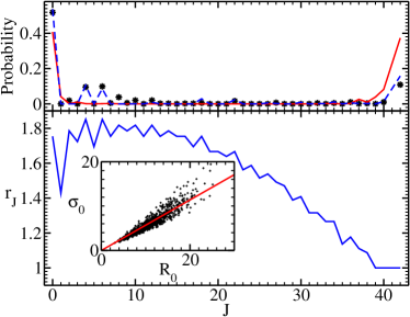
Figure 1: (Color online) 6 fermions in a shell with spin $j=19/2$. Top: Probability that the ground state has spin $J$ (data points); probability that spin $J$ has the largest spectral width (solid line); probability that the product $r_{J}\sigma_{J}$ is maximal (dashed line). Bottom: Scaling factor $r_{J}$ between the widths and spectral radii. Inset: Spectral radius $R_{0}$ versus width $\sigma_{0}$ (data points) and the linear fit (line) for total spin $J=0$. (Results from 900 random realizations).

The two-body random ensemble (TBRE). We consider the Hamiltonian matrix $H(J)$ in the $d_{J}$-dimensional Hilbert space ${\cal H}(J)$ of $n$-fermion states with spin $J$ for a given two-body interaction. The latter has reduced matrix elements (TBME) $v_{\alpha},\alpha=1,\ldots,a$. In our model system, there are $a=10$ TBME since two fermions can have spins $j_{\alpha}=0,2,4,\ldots,2j-1$. The matrix $H(J)$ is linear in the TBME,

$$H(J)=\sum_{\alpha}^{a}v_{\alpha}C_{\alpha}(J)\ .$$ (1)

The matrices $C_{\alpha}(J)$ transport the two-body interaction into the Hilbert space ${\cal H}(J)$. These matrices are determined entirely by the geometry of the shell model. They are built of coefficients of fractional parentage and angular-momentum coupling coefficients.

In order to obtain generic results, we assume that the TBME are uncorrelated Gaussian-distributed random variables with zero mean and unit variance, $\overline{v_{\alpha}}=0$ and $\overline{v_{\alpha}v_{\beta}}=\delta_{\alpha\beta}$ where the bar denotes the ensemble average. Our results then apply to almost all two-body interactions, the integration measure being the product of the differentials of all the $v_{\alpha}$’s. The matrices $H(J)$ are sums of random variables and, thus, form a random-matrix ensemble, the two-body random ensemble. For spins $J\neq J^{\prime}$, the matrices $H(J)$ and $H(J^{\prime})$ depend on the same random variables $v_{\alpha}$ and are thus correlated.

Distribution of spectral widths. The spectral width $\sigma_{J}$ of the states with spin $J$, a random variable, is defined as

$$\sigma_{J}^{2}=d_{J}^{-1}\ {\rm Tr}(H^{2}(J))=\sum_{\alpha\beta}v_{\alpha}S_{\alpha\beta}v_{\beta}\ .$$ (2)

Here $S_{\alpha\beta}(J)=d_{J}^{-1}{\rm Tr}(C_{\alpha}(J)C_{\beta}(J))$ is the symmetric and positive semi-definite $a$-dimensional overlap matrix in the space of the random variables $v_{\alpha}$. Diagonalization of $S=Us^{2}U^{T}$ yields the eigenvalues $s_{1}^{2}(J)\geq s_{2}^{2}(J)\geq\ldots\geq s_{a}^{2}(J)\geq 0$ and the orthogonal, $J$-dependent matrix $U$. The matrices-in-Hilbert-space $B_{\alpha}(J)=\sum_{\beta}U_{\beta\alpha}C_{\beta}(J)$ are orthogonal to each other in the sense of the trace, i.e., $d_{J}^{-1}{\rm Tr}(B_{\alpha}(J)B_{\beta}(J))=\delta_{\alpha\beta}s^{2}_{\alpha}(J)$, and $B_{\alpha}$ has the spectral width $s_{\alpha}$. In terms of the $B$s, the Hamiltonian reads

$$H(J)=\sum_{\alpha}w_{\alpha}B_{\alpha}(J)\ .$$ (3)

The new Gaussian random variables $w_{\alpha}=\sum_{\beta}v_{\beta}U_{\beta\alpha}$ obey $\overline{w_{\alpha}}=0$ and $\overline{w_{\alpha}w_{\beta}}=\delta_{\alpha\beta}$. For fixed $J$, the random-matrix model (3) is equivalent to the random-matrix model (1).

In the new basis, we have

$$\sigma_{J}^{2}=\sum_{\alpha}w_{\alpha}^{2}s^{2}_{\alpha}(J).$$ (4)

The geometric aspects of the shell model are contained in the roots $s_{\alpha}\geq 0$ of the eigenvalues. Figure 2 shows how the $s_{\alpha}$ vary with spin $J$ for our model system. For each spin $J$ there is one particularly large root $s_{1}$. This root increases almost monotonically with $J$. For each spin there is one basis vector $B_{a}(J)$ with root zero. This vector is given by the matrix representation of $\hat{J}^{2}-J(J+1)$ where $\hat{J}$ denotes the spin operator. Indeed, $\hat{J}^{2}-J(J+1)$ annihilates states with spin $J$ and is a scalar two-body operator. Hence, the matrix representation of $\hat{J}^{2}-J(J+1)$ is a linear combination of the matrices $C_{\alpha}(J)$ and, at the same time, an eigenvector of $S_{\alpha\beta}$ with eigenvalue zero. For large values of $J$, there is more than one zero eigenvalue. This is because here the number of independent matrix elements is smaller than the number of TBME.

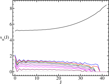
Figure 2: (Color online) Roots of the ten eigenvalues of the eigenvectors $B_{\alpha}(J)$ versus $J$ for 6 fermions in a $j=19/2$ shell.

We first use Fig. 2 for a qualitative discussion of the distribution of widths in the TBRE. Clearly, $\overline{\sigma_{J}^{2}}=\sum_{\alpha}s^{2}_{\alpha}$ attains its maximum value for maximum spin $J=J_{\rm max}$. Among the low spins, $\overline{\sigma_{0}^{2}}$ dominates because the root $s_{1}$ is almost constant for low spins, and the remaining non-zero roots are exceptionally large for $J=0$. As for the fluctuations, we use two limiting cases for orientation: (i) All roots are equal to $s^{2}$. Then $\overline{\sigma^{2}}=as^{2}$ and the r.m.s. variance is $\sqrt{2a}s^{2}$. (ii) Only the root $s_{1}$ differs from zero. Then $\overline{\sigma^{2}}=s^{2}_{1}$ and the r.m.s. variance is $\sqrt{2}s^{2}_{1}$. Thus, we expect that in relation to the average width, the r.m.s. fluctuations of $\sigma_{0}$ are smaller than those of the $\sigma_{J}$ for large $J$.

For a quantitative analysis, we define the probability distribution $P_{J}(\sigma)=2\sigma\overline{\delta(\sigma^{2}-\sigma_{J}^{2})}$ for finding a value of the width between $\sigma$ and $\sigma+{\rm d}\sigma$. The factor $2\sigma$ stems from the differential ${\rm d}\sigma^{2}=2\sigma{\rm d}\sigma$. For $J=J_{\rm max}$ there is only one non-zero root $s_{1}$, and $P_{J_{\rm max}}$ is a Gaussian with width $s_{1}$. For general $J$, all the integrations over the $w_{\alpha}$’s can be done, and the expression for $P_{J}(\sigma)$ reduces to

$$P_{J}(\sigma)={\sigma\over\pi}\int\limits_{-\infty}^{\infty}{\rm d}te^{it\sigma^{2}}\prod_{\alpha=1}^{a}\frac{e^{-{i\over 2}\arctan{2ts^{2}_{\alpha}}}}{\left(1+4s_{\alpha}^{4}t^{2}\right)^{1/4}}\ .$$ (5)

Figure 3 shows $P_{J}(\sigma)$ for several spins $J$. This agrees very well with the histograms from 900 realizations of our TBRE.

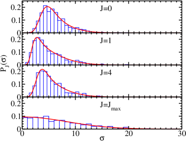
Figure 3: (Color online) Normalized probability distribution functions $P_{J}(\sigma)$ versus spectral width $\sigma$. The histograms result from 900 random realizations for 6 fermions in a $j=19/2$ shell. The line shows the theoretical result (5).

Correlations of widths. The correlations between the Hamiltonian matrices $H(J)$ and $H(J^{\prime})$ induce correlations between the widths $\sigma_{J}$ and $\sigma_{J^{\prime}}$. This fact is borne out by the numerical simulation: Under the assumption that width correlations can be neglected, we can use the distributions $P_{J}(\sigma)$ to compute the probability that spin $J$ has a larger width than spin $J^{\prime}$. Such a calculation yields, e.g., that $\sigma_{0}>\sigma_{4}$ with 60% probability. The numerical simulation of the TBRE shows, however, that $\sigma_{0}>\sigma_{4}$ for 93% of all realizations. Hence, there must be strong correlations between the widths.

We again begin with a qualitative analysis. Let $|u_{J}\rangle$ denote that eigenvector of the overlap matrix $S_{\alpha\beta}(J)$ which corresponds to the largest root $s_{1}(J)$. Figure 4 shows the scalar products $\langle u_{J}|u_{J^{\prime}}\rangle$ as functions of $J-J^{\prime}$. Clearly, the eigenvectors $|u_{J}\rangle$ depend only very weakly on $J$ and are almost identical for total spins that differ by just a few units. In particular, $\langle u_{J}|u_{J^{\prime}}\rangle$ decreases very slowly with $J$ for $J^{\prime}=0$ (upper line in Fig. 4) while the decrease is faster for $J=J_{\rm max}$ (lower line in Fig. 4). We see that for low spins up to values of 10 to 20, the eigenvector of the largest root and the largest root itself are almost independent of $J$. Because of these strong correlations among roots of low spins, the contributions of the largest roots $s_{1}$ to the widths are simultaneously small or simultaneously large for most realizations of the TBRE. In this way the correlations significantly enhance the probability that spin $J=0$ has the largest total width among all low spins. Similar arguments show that the maximum spin $J=J_{\rm max}$ is most likely to exhibit the largest width for high spins. These statements are in keeping with the numerical results presented in the upper part of Fig. 1.

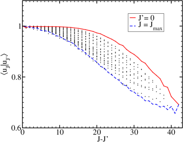
Figure 4: (Color online) Data points: Values of the scalar products $\langle u_{J}|u_{J^{\prime}}\rangle$ of the largest-width eigenvectors $|u_{J}\rangle$ of the overlap matrices $S_{\alpha\beta}=d_{J}^{-1}{\rm Tr}(C_{\alpha}(J)C_{\beta}(J))$ for $J\geq J^{\prime}$. The upper and lower line connect the data points corresponding to $J^{\prime}=0$ and $J=J_{\rm max}$, respectively.

For quantitative results, we define the probability $p(J,J^{\prime})=\overline{\Theta\left(\sigma_{J}^{2}-\sigma_{J^{\prime}}^{2}\right)}$ that spin $J$ has a larger width than spin $J^{\prime}$, where $\Theta$ denotes the unit step function. Introducing the eigenvalues $q_{\alpha}$ of the matrix $S_{\alpha\beta}(J)-S_{\alpha\beta}(J^{\prime})$, we can perform the ensemble average. Employing integral transforms, we arrive at

$$p(J,J^{\prime})={1\over 2}+{1\over\pi}\int\limits_{0}^{\infty}{\rm d}t{\sin{\left({1\over 2}\sum_{\beta}\arctan{2tq_{\beta}}\right)}\over t\prod_{\alpha}\left(1+4q_{\alpha}^{2}t^{2}\right)^{1/4}}\ .$$ (6)

This expression accurately describes the results of our numerical simulation.

From widths to ground states. The bridge between the spectral widths discussed so far and the spin of the ground state is spanned by the scaling factors $r_{J}$. These are defined as follows. For each value of $J$, every realization of the TBRE yields a spectrum $E_{J,i},i=1,\ldots,d_{J}$. Let $R_{J}=\max_{i}|E_{J,i}|$ be the spectral radius for spin $J$. For each realization, $R_{J}$ is given with equal probability either by the energy of the lowest-lying level or by that of the highest-lying level with spin $J$. The spectral radius is related to the spectral width $\sigma_{J}$ of that realization by the inequality $R_{J}\geq\sigma_{J}$. However, our numerical results show that the much stronger relation

$$R_{J}\approx r_{J}\ \sigma_{J}$$ (7)

is approximately valid, with $r_{J}$ constant (independent of the realization considered). This is shown in the inset of Fig. 1. The scaling factor $r_{J}\geq 1$ (shown in the lower part of Fig. 1) encodes information contained in the tails of the spectral density. The average level density typically decreases exponentially fast for energies close to the spectral radius. Thus, $r_{J}$ is expected to exhibit only a logarithmically weak dependence on the dimension $d_{J}$ and on the average width. We neglect this dependence as well as the difference between the absolute values of the energies of the highest and the lowest level in the spectrum of each realization. Thus, we identify the product $r_{J}\sigma_{J}$ with the energy of the lowest-lying state with spin $J$. It is then tempting to assume that the probability distribution of $R_{J}$ is simply given by that of $\sigma_{J}$ scaled by the factor $r_{J}$. Our numerical results show, however, that the two distributions, although similar, do not really coincide. However, the relation (7) is sufficiently accurate to determine reasonably reliably the probability that $r_{J}\sigma_{J}$ is maximal. Indeed, this probability is plotted as the dashed line in the upper part of Fig. 1. The agreement with the data points is very satisfactory.

We have obtained similar results for $n=8$ fermions in a $j=19/2$ shell. For the odd-number system with $n=7$, we also found that minimum and maximum spins are most likely to exhibit the largest widths. However, other spins also have smaller but sizable probabilities of having the largest widths.

Summary. We have studied the spin of the ground state for the shell model with random two-body interactions. To this end, we have derived closed expressions for both, the width distribution functions and the width correlation functions. Using these results, we have shown that spin-0 and maximum spin are most likely to exhibit the largest widths. The spin-0 width is characterized by a relatively large average value and rather small fluctuations, while the maximum spin displays the largest average and the largest fluctuations. We have numerically established an approximate proportionality between spectral widths and spectral radii. This relation is sufficiently reliable to explain the preponderance of spin-0 ground states in the shell model.

This work has been confined to a single shell with spin $j=19/2$. However, our results depend only upon geometrical properties of that model and are thus expected to apply similarly in other shells. We speculate that similar considerations would also apply to other many-body systems.

The distribution functions were calculated using superpositions of two-body operators whose squared widths sum up to the average spectral width of the random Hamiltonian. These operators may have further applications in nuclear structure calculations: Effective interactions are often obtained from fitting two-body matrix elements Honma02 . These procedures ideally should avoid generating linear combinations of two-body operators with small or zero spectral widths.

Our work poses the intriguing analytical problem to derive the eigenvalues $s_{\alpha}(J)$. These are determined entirely by the geometry of the shell model. Hence, the values of the $s_{\alpha}(J)$ should be accessible by group-theoretical techniques. An understanding of the scaling factors $r_{J}$ seems less difficult. It would require the knowledge of the shapes of the average spectra. This would allow us to determine $r_{J}$ from the position of the lowest level (found by integrating the normalized spectrum from $-\infty$ to where the integral equals $1/2$) and the width of that spectrum.

This research was supported in part by the U.S. Department of Energy under Contract Nos. DE-FG02-96ER40963 (University of Tennessee) and DE-AC05-00OR22725 with UT-Battelle, LLC (Oak Ridge National Laboratory).

References

- (1) C. W. Johnson, G. F. Bertsch, and D. J. Dean, Phys. Rev. Lett. 80, 2749 (1998), nucl-th/9802066.
- (2) R. Bijker and A. Frank, Phys. Rev. Lett. 84, 420 (2000), nucl-th/9911067.
- (3) P. Jacquod and A. D. Stone, Phys. Rev. Lett. 84, 3938 (2000), cond-mat/9909067.
- (4) V. Zelevinsky and A. Volya, Phys. Rep. 391, 311 (2004), nucl-th/030907.
- (5) Y. M. Zhao, A. Arima, N. Yoshinaga, nucl-th/0311050.
- (6) D. Kusnezov, Phys. Rev. Lett. 85, 3773 (2000), nucl-th/0009076.
- (7) Y. M. Zhao and A. Arima, Phys. Rev. C64, 041301(R) (2001), nucl-th/0108052.
- (8) P. Chau Huu-Tai, A. Frank, N. A. Smirnova, and P. Van Isacker, Phys. Rev. C66, 061302(R) (2002), nucl-th/0301061.
- (9) R. Bijker and A. Frank, Phys. Rev. C64 , 061303 (2001), nucl-th/0111009.
- (10) R. Bijker, A. Frank, and S. Pittel, Phys. Rev. C60, 021302 (1999), nucl-th/9906046.
- (11) L. Kaplan, T. Papenbrock, and C. W. Johnson, Phys. Rev. C63, 014307 (2001), nucl-th/0007013.
- (12) V. Velázquez and A. P. Zuker, Phys. Rev. Lett. 88, 072502 (2002), nucl-th/0106020.
- (13) T. Papenbrock, L. Kaplan, and G. F. Bertsch, Phys. Rev. B65, 235120 (2002), cond-mat/0202493.
- (14) V. K. B. Kota and K. Kar, Phys. Rev. E65, 026130 (2002).
- (15) N. Yoshinaga, A. Arima, and Y. M. Zhao, J. Phys. A 35, 8575 (2002).
- (16) D. Mulhall, A. Volya, and V. Zelevinsky, Phys. Rev. Lett. 85, 4016 (2000), nucl-th/0005014.
- (17) Y. M. Zhao, A. Arima, and N. Yoshinaga, Phys. Rev. C66, 034302 (2002), nucl-th/0112075.
- (18) M. Honma, B. A. Brown, T. Mizusaki, and T. Otsuka, Nucl. Phys. A704, 134c (2002).