Precise study of the Efimov three-particle spectrum
and structure functions within variational approach

Abstract

A precise study within variational approach of the basic properties of the three-particle spectrum and structure functions with Gaussian potential near the critical coupling constant of interaction where the Efimov effect takes place is carried out. A method is developed to calculate highly excited states with very small binding energies, and numerical analysis is carried out for the ground and three excited energy states. For these states, one-particle density distributions, formfactors, pair correlation functions, and momentum distributions are calculated. It is found that the second excited state has already all the basic features of a level from the infinite Efimov series. An essential asymmetry is found in the position of energy levels with respect to the critical constant point. A halo-type structure is revealed in the one-particle density distributions, and formfactors are shown to have specific dips of finite depth, the number of dips being equal to the number of the state. The behaviour of pair correlation functions and momentum distributions is studied for three-particle states.

I Introduction

As known, the Efimov effect R1 ; R2 ; R3 reveals itself in a system of three particles with finite-range interaction as the appearance of the infinite number of levels near the threshold with very small energies under the condition that the two-particle subsystems have an infinitely small binding energy or an infinitely large scattering length. In the case of three identical particles, the energy ratio for neighboring highly excited near-threshold Efimov states R1 ; R4 is $\lambda_{E}=\lim\limits_{n\to\infty}(E_{n}/E_{n+1})\approx 515$. In three-nucleon systems, the conditions necessary for the effect to take place can be easily broken by taking into account the spin structure of the nuclear interaction R3 ; R6 or the Coulomb long-range repulsive potential.

Theoretical studies of the Efimov near-threshold energy spectrum were carried out both by asymptotic expansions with the use of the small parameter $r_{0}/a\ll 1$ (being the ratio of the range of forces to the two-particle scattering length) R1 ; R2 ; R3 ; R5 ; R6 and by numerical calculations R7 ; R8 based on the Faddeev equations by using separable interaction potentials. The main properties of the energy states are universal to the great extent and do not depend on a specific form of the potential. For the special choice of an interaction potential in the form of two components with essentially different radii, new additional excited energy levels appear in the three-particle system — the “trap” effect R9 . In the case of local potentials, numerical calculations of the Efimov energy spectrum were not carried out systematically because of essential difficulties due to the different scales of very small near-threshold excited states energies and the ground-state energy. This requires to develop the precise methods of calculation of the highly excited weakly bounded states of three-particle systems with local interactions.

Due to the use of Gaussian bases in the variational calculations of a few-particle systems R10 , noticeable progress was achieved in the calculations of the main properties of few-body systems R11 ; R12 ; R13 ; R14 with interactions of different nature in recent years. In the present paper, within the precise variational approach, a study of the near-threshold Efimov states of a three-particle system with Gaussian potential is carried out up to the third excited level, and all the main structure functions for various energy states are found.

II Statement of the Problem

Consider a system of three identical particles

$$H=-\frac{\hbar^{2}}{2m}\sum\limits_{i=1}^{3}\Delta_{i}-V_{0}\sum\limits_{i>j=1}^{3}\exp\left(-\frac{r_{ij}^{2}}{r_{0}^{2}}\right)$$ (1)

with a two-particle interaction taken in the Gaussian form for simplicity, where $V_{0}$ is the intensity and $r_{0}$ is the radius of forces. Let us study the properties of the energy spectrum and the main structure functions of the system in symmetric (with respect to permutations of particles) states with zero total angular momentum in the range of parameters where the Efimov effect takes place. It is convenient to use the dimensionless variables and to measure all the distances in $r_{0}$ and energies in $\hbar^{2}/mr_{0}^{2}$. In this case, the dimensionless Hamiltonian

$$H=-\frac{1}{2}\sum\limits_{i=1}^{3}\Delta_{i}-g\sum\limits_{i>j=1}^{3}\exp\left(-r_{ij}^{2}\right)$$ (2)

contains only one combination of physical parameters, the coupling constant $g=mr_{0}^{2}V_{0}/\hbar^{2}$, which determines the properties of the spectrum and wave functions of the system.

The solution of the problem on eigenvalues and eigenfunctions for bound states is carried out in the framework of the variational Galerkin method in the Gaussian representation with the use of special optimization schemes (see R12 ; R13 ; R14 ) which enhance the convergence and ensure a high accuracy of calculations with the least dimensions of variational bases. Within this approach, the variational wave function of symmetric states of the three-particle system with zero total angular momentum can be presented as the expansion in Gaussian functions depending on relative distances $r_{ij}=\left|{\bf r}_{i}-{\bf r}_{j}\right|$,

$$\Psi\left(r_{12},r_{13},r_{23}\right)=\sum\limits_{k=1}^{\cal K}{D_{k}{\bf S}\left.\left|{\psi_{k}}\right.\right\rangle}\equiv\sum\limits_{k=1}^{\cal K}{D_{k}{\bf S}\exp\left(-a_{k}r_{12}^{2}-b_{k}r_{13}^{2}-c_{k}r_{23}^{2}\right)}\,,$$ (3)

with a set of variational parameters $a_{k}$, $b_{k}$, $c_{k}$. For the bound states, the linear coefficients $D_{k}$ are found in the variational approach from the system of linear algebraic equations of a problem on eigenvalues (which is equivalent to the Schrödinger equation in the chosen Gaussian basis):

$$\sum\limits_{n=1}^{\cal K}D_{n}\Bigl{(}\left\langle{\bf S}\psi_{k}\left|H\right|{\bf S}\psi_{n}\right\rangle-E\left\langle{\bf S}\psi_{k}\left|{\bf S}\psi_{n}\right.\right\rangle\Bigr{)}=0,\,\,\,k=1,2,\dots,{\cal K}.$$ (4)

Note that all the matrix elements in Eq. (4) for Hamiltonian (2) can be calculated in explicit form. The chosen method of calculation has proved its high efficiency and accuracy in a number of problems of a few particles with interactions of different nature. But, in the case of the near-threshold Efimov spectrum, we are faced with an additional difficulty due to very small values of the energies of these levels. Since the ratio of the Efimov neighboring energy levels $\lambda_{E}=\lim\limits_{n\to\infty}(E_{n}/E_{n+1})\approx 515$ is rather large, there exists a real difficulty for all the methods (including the method based on the Faddeev equations R9 and variational methods as well) in calculating the energies with essentially different scales and the corresponding wave functions with oscillations at essentially different distances.

In the present work, the main structure properties of the ground and three excited states of a system of three particles are calculated with the coupling constants near $g\approx g_{cr}$, where a two-particle bound state appears and the Efimov effect reveals itself. The numerical analysis of highly excited near-threshold Efimov levels appears to be a nontrivial problem for all the methods including the variational method because of the necessity to prepare the “initial” configurations for the wave functions of highly excited near-threshold bound states to start the minimization of energy in the nonlinear variational parameters $a_{k}$, $b_{k}$, $c_{k}$.

III The Problem of Initial Configurations

An advantage of the variational method lies in the possibility to calculate (in the approximation of a given number of the basis functions) the whole spectrum of low-energy bound states for a given Hamiltonian or to calculate the energy and wave function of the chosen ground or excited state separately. The further minimization in the nonlinear parameters $a_{k}$, $b_{k}$, $c_{k}$ enables one to improve the variational estimation for the energy and to achieve the best result at a fixed dimension of the basis in (3). It is clear that if the initial configuration gives, in fact, the bound (ground or excited) state, we have to approach the exact solution for this state by minimizing the nonlinear parameters $a_{k}$, $b_{k}$, $c_{k}$ and expanding the basis dimension. However, at a finite and even rather large number ${\cal K}$ of the basis functions in (3) and with a random set of the nonlinear parameters $a_{k}$, $b_{k}$, $c_{k}$ (we call it a random “initial configuration”), nobody can be sure not only in the fact that the studied energy level is close to the exact value, but, even more, that it is below the threshold of a decomposition into subsystems at all. In the latter case, as a rule, the further minimization in nonlinear parameters should be terminated on approaching the rated level to the threshold (from the side of the continuum spectrum), because the wave function can have nothing in common with a bound state. Such problems reveal themselves starting from the second excited state which exists in a narrow interval near $g\approx g_{cr}=2.684005$ (the critical constant for the chosen Gaussian potential). There is no such problem for the ground state of three particles, whose initial configuration can be simply prepared even with one Gaussian function at sufficienly large $g$. The mentioned problem is also easily solved for the first excited state if one takes several Gaussian functions, among which at least two or three ones depend on the parameters $a_{k}$, $b_{k}$, $c_{k}$ taken from the ground-state function, while the rest have to form a cluster function R13 . This enables one to rather simply construct the necessary configuration (even in the case where the initial configuration corresponds to an energy slightly exceeding the two-particle threshold). For the ground and first excited states, the problem is simplified also due to the fact that these levels exist at all the interaction constants $g$ greater than certain critical values (see Table 1). Therefore, it is sufficient to enhance the attractive potential, to form the initial configurations at a sufficiently large $g$, and then, by gradually decreasing $g$ (the evolution in coupling constant), to achieve the necessary value of $g$ by minimizing the energy in the parameters $a_{k}$, $b_{k}$, $c_{k}$. We used both variants to form the initial configurations for the ground and first excited states.

For the following excited near-threshold Efimov states with extremely small binding energies existing within a narrow interval of $g$ near the critical two-particle constant $g_{cr}$, the problem of initial configurations requires special methods for its solution. One way is to use a wider class of Hamiltonians, in particular, those with an additional interaction giving a possibility to form relatively easily the configurations of highly excited levels. Then the above interaction is eliminated step by step (in order to return to the initial problem) with a simultaneous change in the parameters $a_{k}$, $b_{k}$, $c_{k}$ within the variational procedure in order to keep the energies of the formed configurations below the threshold. The Coulomb attractive interaction seems to be suitable for this purpose giving rise to the infinite number of levels for the three-particle system. An additional advantage of this interaction is the fact that all matrix elements in the Gaussian basis for the Coulomb potential are known to be calculated in explicit form.

Another way to prepare the initial configurations is to deal with a Hamiltonian with different masses of particles. It is known that the Efimov effect takes place in three-particle systems with different masses R1 ; R2 ; R3 . Moreover, the ratio of the energies of neighboring levels depends significantly on the ratio of masses (see also R15 ). From the analysis of the power asymptotics of a three-particle wave function in the momentum representation within the approach based on the Faddeev equations, it can be shown that the following secular equation is the condition for the solvability of three-particle equations:

$$L(1;2,3)L(2;1,3)+L(1;3,2)L(3;1,2)+L(2;3,1)L(3;2,1)+$$

$$L(1;3,2)L(2;1,3)L(3;2,1)+L(1;2,3)L(2;3,1)L(3;1,2)=1;$$ (5)

where

$$L(i;j,k)\equiv N(\frac{\mu_{jk}}{\mu_{i}};\frac{\mu_{jk}}{m_{k}});\,\,\,N(a;\,b)\equiv\frac{\sinh(s_{0}\theta/2)}{b\sqrt{a}\,s_{0}\,\cosh(s_{0}\pi/2)};\,\,\,\cos\theta\equiv\frac{a-b^{2}}{a+b^{2}};$$ (6)

$$\mu_{jk}\equiv\frac{m_{j}m_{k}}{m_{j}+m_{k}};\,\,\,\mu_{i}\equiv\frac{m_{i}(m_{j}+m_{k})}{m_{i}+m_{j}+m_{k}}.$$ (7)

In the case of equal masses, the secular equation (5) becomes essentially simpler R1 :

$$N\left(\frac{3}{4};\,\frac{1}{2}\right)=\frac{1}{2}\,,$$ (8)

or

$$\frac{8}{\sqrt{3}}\,\frac{\sinh(\pi s_{0}/6)}{s_{0}\cosh(\pi s_{0}/2)}=1\,,$$ (9)

and one has for the power $s_{0}$ of the asymptotics of the Faddeev equations solution (the Danilov-Minlos-Faddeev-Efimov constant), $s_{0}=1.0062378$. This constant determines, in particular, the ratio of Efimov neighboring energy levels (the scale invariance multiplier),

$$\lambda_{E}=\lim\limits_{n\to\infty}(E_{n}/E_{n+1})=\exp\left(\frac{2\pi}{s_{0}}\right)\cong 515.035\,.$$ (10)

Fig. 1 shows the dependence of the ratio $\lambda_{E}=\exp(2\pi/s_{0})$ of the energies of Efimov neighboring levels on the ratio of the masses of particles. It is seen clearly that the case of equal mases is the most unsuitable for the Efimov effect to reveal itself (the scale multiplier $\lambda_{E}$ is the greatest) and, at the same time, it is the most difficult case for numerical calculations. But, in the case of essentially different masses, one may have the ratio of energies not too far from 1 instead of (10) (for any ratio of masses, of course, we have $\lambda_{E}>1$ ). In particular, in the limit $m_{1}/m_{3}=m_{2}/m_{3}\to 0$ (the one-center problem), relation (5) yields the limiting secular equation for $s_{0}$:

$$\left\{1+8\left[1+\cosh^{-1}\left(\frac{s_{0}\pi}{2}\right)\right]\left[\sinh\left(\frac{s_{0}\pi}{4}\right)/s_{0}\right]^{2}\right\}\cosh^{-2}\left(\frac{s_{0}\pi}{2}\right)=1\,.$$ (11)

This results in $s_{0}=1.139759$, and the corresponding ratio of energies $\lambda_{E}=247.826$. If, vice versa, $m_{1}/m_{3}=m_{2}/m_{3}\to\infty$ (the two-center problem), the value of $s_{0}$ increases infinitely as $s_{0}\to k\sqrt{m_{1}/m_{3}}$, where the coefficient $k=0.40103$ is found from the secular equation

$$\frac{\exp(-k\sqrt{2})}{k\sqrt{2}}=1\,.$$ (12)

The corresponding ratio of energy levels goes to 1 as $\lambda_{E}\to 1+\frac{2\pi}{k}\sqrt{\frac{m_{3}}{m_{1}}}$ at $m_{3}/m_{1}\to 0$. It should be noted that, due to the essential dependence of the parameter $\lambda_{E}$ on the ratio of masses, it is more probable to observe the Efimov effect in a real physical system just with different masses of particles whose pairwise interaction is of the resonance type. Close to such systems might be three-cluster nuclei consisting of a rather heavy magic core and two neutrons. In particular, if the nucleus ⁴⁰Ca serves to be the core, it follows from (5) that $\lambda_{E}\approx 262$ (i.e., it is twice smaller than that for equal masses). If, to say, we consider the system of mesoatoms of deuterium and tritium interacting with an electron, then, due to the small mass of an electron in comparison with the masses of mesoatoms, one has a large value of $s_{0}$ from (5) enough to result in $\lambda_{E}\cong 1.26$. This value is not essentially greater than 1 and much less than that in the case of equal masses. This means that the energies of neighboring Efimov levels would be of the same order of magnitude if they were observed in such a system.

Returning to the problem of formation of initial configurations, we note that the configuration for a given (the $n$-th excited) state can be prepared rather easily at different masses. Then one has to restore step by step the equality of masses by minimization of the energy of this level in nonlinear parameters. In this way, we can get the necessary variational wave function corresponding to the configuration of a bound state.

To obtain the initial configurations for variational wave functions, we paid the main attention to the method of evolution in the coupling constant $g$ at a fixed (zero) energy, which is possible because the interaction potential in (1) has a definite sign. The method, in essence, consists in a variational procedure with respect to the critical coupling constant $g$ to be determined for the given ground or excited state at a fixed (zero) energy. It is the general statement that the variational method can be formulated with respect to the coupling constant $g$ at a fixed energy provided that the interaction potential is negative definite. Taking an arbitrary initial configuration with a sufficient number of the basis functions with some parameters $a_{k}$, $b_{k}$, $c_{k}$, we find the corresponding coupling constant $g$ of the chosen excited state by variational procedure and advance step by step towards small $g$ by varying the parameters $a_{k}$, $b_{k}$, $c_{k}$ (or sometimes, if necessary, by spreading the basis). Thus, we approach the two-particle critical constant from the upper side, where a two-particle ground state appears. When we are close enough to the region $g\approx g_{cr}$, where the Efimov excited state under consideration must exist, we return to the commonly used variational procedure in energy using the obtained set of the parameters $a_{k}$, $b_{k}$, $c_{k}$ and start to increase the parameter $g$. If we were close enough to the critical constant $g_{cr}$, the three-particle energy level crosses the two-particle threshold and goes down below the threshold. Thus, we obtain the required initial configuration. Such a possibility is connected with the fact that the two-particle energy threshold behaves itself by the square law near the critical coupling constant,

$$E_{(2)}\cong-\,0.107\,(g-g_{cr})^{2}\,,$$ (13)

while three-particle levels reveal a linear behavior R1 ,

$$E_{n}\cong k_{n}\,(g-g_{left}^{(n)})\,,$$ (14)

where $g_{left}^{(n)}$ is the critical constant for the $n$-th level appearance on the left from the critical constant, and $k_{n}=\partial E_{n}/\partial g$ (at the critical point $g=g_{left}^{(n)}$) is the corresponding angular coefficient (see Table 1). Using the above method, we succeeded in preparing the initial configurations for the second and third excited states which exist near the critical constant $g_{cr}$ and belong to the Efimov series of levels. Note that the greater the number of the excited near-threshold Efimov level, the greater are the difficulties in preparing the initial configuration. It is not only due to the necessity to increase the dimension of the variational basis, but also because the nonlinear variational parameters differ from one another by several orders of magnitude. Moreover, there appears a considerable quantity of nonlinear parameters such that they are roughly by $\lambda_{E}$ times smaller than those typical of the previous energy level. This makes it necessary to significantly decrease the steps in the process of variation in nonlinear parameters and decelerates the whole procedure of preparing the initial configuration. Because the energy of already the third excited level is less by nine orders of magnitude in comparison with the ground state energy and the dimension of the basis which is necessary to ensure a reliable accuracy achieves several hundreds of functions, the calculation of levels higher than the third one becomes a serious problem.

IV Asymmetry of the Efimov Energy Levels

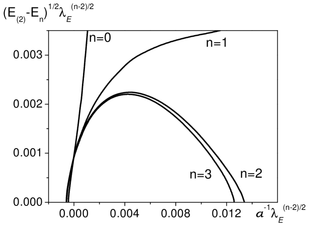
Figure 2: Dependence of $(E_{(2)}-E_{n})^{1/2}$ on the reciprocal scattering length $a^{-1}$ for the ground ($n=0$) and excited ($n=1,2,3$) states. Each of the levels is depicted on another scale with the use of the multiplier $\lambda_{E}^{(n-2)/2}$ for both axes.

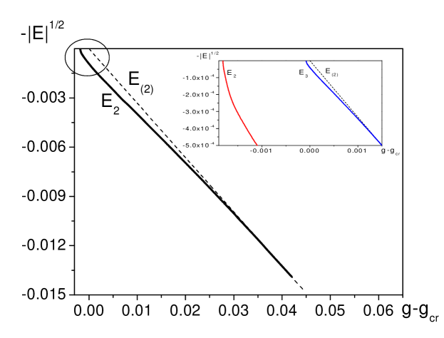
Figure 3: Dependence of the second and third excited energy levels on the coupling constant $g$. The third excited level is shown in the enlarged fragment.

It is convenient to depict the calculated energies of the ground and excited states of a three-particle system as the square roots of the moduli of three-particle energies minus the two-particle energy threshold versus the reciprocal scattering length (instead of the coupling constant $g$), because such dependences are model-independent R1 ; R2 ; R3 ; R5 to the great extent. Since the orders of magnitude of the values (of both energies and reciprocal scattering lengths) are essentially different for different levels (the ratio for neighboring levels being about $\sqrt{\lambda_{E}}=\exp(\pi/s_{0})=22.692$ ), Fig. 2 shows each level in its own scale in order to emphasize the universal properties of highly excited states. Namely, the horizontal axis depicts $a^{-1}\lambda_{E}^{(n-2)/2}$, and the vertical axis shows $(E_{(2)}-E_{n})^{1/2}\lambda_{E}^{(n-2)/2}$. The ground and first excited states exist at any $g$ greater than the corresponding critical values (see Table 1). The reciprocal scattering length $a^{-1}$ is approximately proportional to $g-g_{cr}$ near the two-particle critical constant $g\cong g_{cr}$. Note that the separation of three-particle levels from the zero energy occurs by law (14), though this linear behavior takes place only in a very narrow interval near the corresponding three-particle critical coupling constant, and the angular coefficient $k_{n}$ decreases essentially with increase in the number of the excited state. The second and third excited states appear with increase in $g$ (in the region $g<g_{cr}$) and then disappear (in the region $g>g_{cr}$) at the two-particle threshold (the corresponding values of the coupling constants $g$ and the reciprocal scattering lengths are given in the second and third columns in Table 1). A rather good coincidence of the curves for the second ($n=2$) and third ($n=3$) excited levels depicted in Fig. 2 testifies to that the asymptotic formulae R1 ; R2 are valid already starting from the second excited state and indicates the fact that highly excited Efimov states possess the scaling property. Although we restricted ourselves by the calculations of only three excited levels, it should be assumed that the rest of levels is to be determined by the asymptotic relations, and thus the properties of the whole spectrum are completely described. A significant asymmetry of the curves obtained in our calculations for the second and third excited states relative to the critical concentration point $g_{cr}$ of the Efimov spectrum testifies to the asymmetry of all the rest levels. Each of them extends to the right side from the critical point much farther than to the left. This essential asymmetry of the levels relative to the point $g=g_{cr}$ (or $a^{-1}=0$) is connected with the following fact. Though the potential of the effective long-range interaction $\sim-R^{-2}$ R1 ; R2 ; R3 ranges up to distances of the order of $\left|a\right|$, it remains attractive at essentially larger distances at $a>0$. Whereas, at $a<0$, it becomes practically zero out of the region of about $\left|a\right|$ (see also R15 ). The above-mentioned asymmetry is clearly seen in Fig. 3, where the second and third excited states are depicted in natural scale versus the coupling constant $g$. This figure contains a fragment of the near-threshold area in larger scale in order to make the third level visible, since it looks almost like a dot and cannot be distinguished from the two-particle threshold within the main figure. Note that the largest binding energy of each of the Efimov levels (minus the energy of the two-particle threshold) happens at the constants rather far from the critical concentration point of the spectrum (see Fig. 2 and Fig. 3), though the infinite number of levels appears only at the limiting point $g_{cr}$. The three-particle levels cross the two-particle threshold (with increase in $g$) at very small angles at the points in Fig. 3, where the solid lines of these levels become the dashed line of the two-particle threshold. After crossing the two-particle threshold, the three-particle levels may exist over the threshold as virtual states (see R16 ). It is worth to note that, with the essential enlargement of the coupling constant $g$ up to $g\geq g_{cr}^{(2)}=16.3$, the second excited level appears below the two-particle threshold, the third one does at $g\geq g_{cr}^{(3)}=30.8$, the fourth does at $g\geq g_{cr}^{(4)}=32.55$, the fifth does at $g\geq g_{cr}^{(5)}=50.89$, and so on. Their binding energies increase with the coupling constant. The angular coefficients determining the angle between the curve of the $n$-th level and the two-particle energy threshold (near the critical point of the corresponding level appearance),

$$E_{n}-E_{(2)}\cong\tilde{k}_{n}\left({g-g_{cr}^{(n)}}\right)\,,$$ (15)

are as follows: $\tilde{k}_{2}\cong-0.0045$, $\tilde{k}_{3}\cong-0.1$, $\tilde{k}_{4}\cong-0.01$, and $\tilde{k}_{5}\cong-0.03$. The fact that, for the third and fourth levels, $g_{cr}^{(3)}$ and $g_{cr}^{(4)}$ are close one to another, as well as that the angular coefficients $\tilde{k}_{3}$ and $\tilde{k}_{4}$ are of different order of magnitude, testifies to a different nature of these levels.

V Structure Functions of the Efimov States

The wave functions of the three-particle ground and excited states calculated within the precise variational approach enable us to calculate directly such structure functions of the system as density distributions, formfactors, pair correlation functions, momentum distributions, etc. It is a rather simple problem to calculate any such an average since the wave functions of each state have the simple form (3) of a superposition of Gaussian functions with the already known linear ($D_{k}$) and nonlinear ($a_{k}$, $b_{k}$, $c_{k}$) parameters.

Fig. 4 presents the one-particle density distributions,

$$n(r)=\left\langle\frac{1}{3}\sum\limits_{i=1}^{3}\delta\left({\bf r}-\left({\bf r}_{i}-{\bf R}_{c.m.}\right)\right)\right\rangle\,,$$ (16)

for the ground and excited states at the critical two-particle coupling constant $g_{cr}$. The density distributions (16) are shown in logarithmic scale on both axes. This is made, on the one hand, in order that the typical “halo” structure appearing for different states at distances of different scales can be shown in the same figure. On the other hand, on the chosen logarithmic scale, the density distributions reveal clearly the almost periodic dependence of the wave functions of Efimov states on the global radius logarithm R1 $\sim\sin\left(\left|s_{0}\right|\ln\left(R\sqrt{m\left|E\right|/\hbar^{2}}\right)+\Delta\right)$. Moreover, this asymptotic behavior is valid from the distances of about the radius of forces (in our case, of about 1) to the distances of about $\hbar\left(m\left|E\right|\right)^{-1/2}$. The less the binding energy of an excited state, the longer is the extension of this asymptotic behavior. The density distribution of the first excited state is seen to change sharply its behavior between the short and long distances. The long-range “halo” is situated around the more condensed central core similar to the density distribution of the ground state. The density distribution of the second excited state changes its behavior two times having a “halo” in the form of two concentric spherical layers put one into another. They are of essentially different radii and densities and have the central part of the same type as in the case of the first excited state. The density distribution of the third excited state changes its behavior three times (three concentric layers around the central core), and so on. The ratio of the radii of neighboring layers is about $\sqrt{\lambda_{E}}\cong 22.7$. Since the density distributions are normalized by $\int n(r)d{\bf r}=1$, they decrease at short distances when the number of the excited state increases, because the size of the system is growing.

The fact that the ratio of the sizes of neighboring states of the system is about $\sqrt{\lambda_{E}}$ is a consequence of the universal model-independent properties of Efimov states and is confirmed once more by calculations of the r.m.s. radii (see Table 1 with the calculated $R_{rms}$ at the critical value $g_{cr}$). Note that the smallest value of $R_{rms}$ for a given Efimov level is achieved at the constant $g$ corresponding to the largest binding energy, rather far to the right from the critical point $g_{cr}$ (see Fig. 2). When the coupling constant approaches the value, where the Efimov levels appear at the threshold ($E\to 0$), the calculated mean square radius

$$R_{rms}\equiv\left\langle{r^{2}}\right\rangle^{1/2}=\left(\int{r^{2}n(r)d{\bf r}}\right)^{1/2}$$ (17)

reveals the behavior

$$\left\langle{r^{2}}\right\rangle^{1/2}=\frac{c_{1}}{\sqrt{E}}+c_{2}+\dots\,.$$ (18)

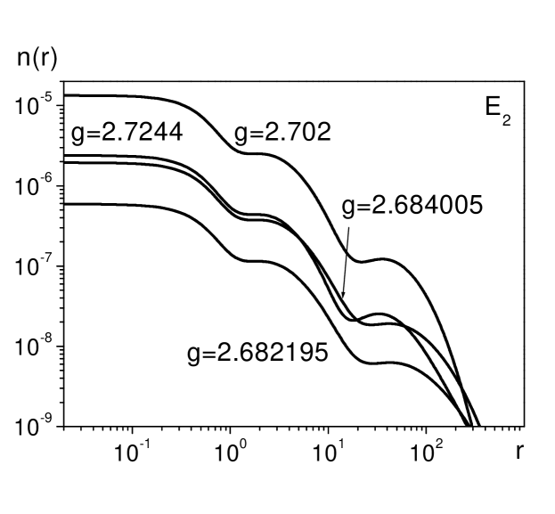
Figure 5: Density distribution profiles with several different coupling constants $g$ for the second excited state.

That is, the radius goes to infinity, in accordance with the general physical principles, as $\left\langle{r^{2}}\right\rangle^{1/2}\sim(E)^{-1/2}$ at $E\to 0$ (we recall that the energy level near the threshold depends linearly on the coupling constant according to (14)). It is important to notice that the growth of the r.m.s. radii at $E\to 0$ is connected mainly with the extension of the region where the asymptotic behavior of the wave function $\sim\sin\left(\left|s_{0}\right|\ln\left(R\sqrt{m\left|E\right|/\hbar^{2}}\right)+\Delta\right)$ is valid, i.e., up to the distances of order $\hbar\left(m\left|E\right|\right)^{-1/2}$. At the same time, the wave function at short and intermediate distances does not change (except for the normalization factor depending on the total size of the system). As a result, in all the intervals of $g$ where a given Efimov level exists, the behavior of the wave function and, in particular, the density distribution is not changed at short and intermediate distances (but only the normalization does), which is confirmed by Fig. 5. This figure shows the density distributions of the second excited state at several different values of the coupling constant, from the point $g=2.682195$ near the level appearance to the point $g_{right}^{(2)}=2.7244$ of its disappearance. Other typical constants chosen by us are as follows: the two-particle critical constant $g_{cr}$ (the point of the Efimov spectrum concentration) and the constant $g=2.702$, where the energy of the second excited state (minus the two-particle threshold energy) is the greatest.

Specific sharp changes in the density profiles near the distances, where the corresponding wave functions pass through zero, manifest themselves in formfactors,

$$F(q)=\int\exp(-i{\bf q}\cdot{\bf r})n(r)d{\bf r}\,,$$ (19)

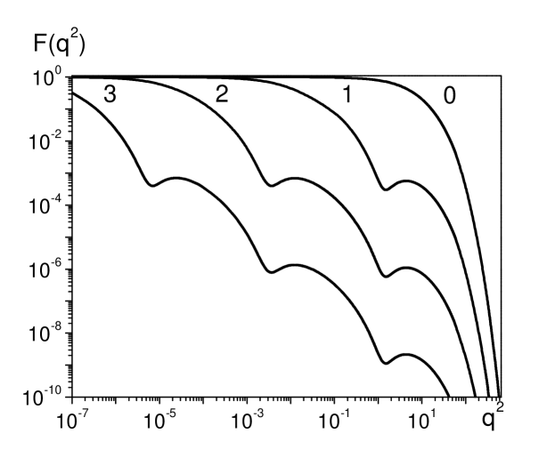
Figure 6: Formfactors for the ground ($n=0$) and three excited ($n=1,2,3$) states.

in the form of specific dips of finite depth. Fig. 6 shows the formfactors of the ground state (no dips), the first (one dip), second (two dips), and third (three dips) excited states. A logarithmic scale commonly used for formfactors on the vertical axis is accomplished with the logarithmic scale in the squared momentum transfer in order to show clearly the almost periodic repetition of the dips connected with regularities in the “halo” structure of the density distributions of excited states. Since the greater distances in a density distribution correspond to a less momentum transfer in the corresponding formfactor and vice versa, a new dip in the formfactor of the next excited state appears at a less momentum transfer, whereas the previous dips remain practically at their positions.

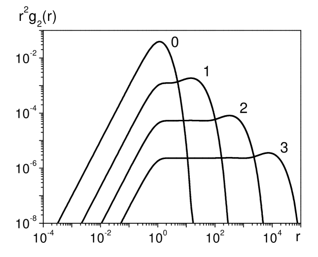
Figure 7: Pair correlation functions for the ground ($n=0$) and three excited ($n=1,2,3$) states.

Fig. 7 shows the pair correlation functions

$$g_{2}(r)=\left\langle\frac{1}{3}\sum\limits_{i>j=1}^{3}\delta\left({\bf r}-\left({\bf r}_{i}-{\bf r}_{j}\right)\right)\right\rangle$$ (20)

of the ground state and three excited states. We multiply the pair correlation functions by $r^{2}$ in order to show clearly the following interesting effect. With increase in the number of the excited state, we observe the spreading of the area, where the pair correlation function is proportional to the reciprocal squared distance between a pair of particles. That is, the two-particle subsystem in the system of three particles has the density distribution very similar to the squared two-particle wave function. This gives rise to the effective long-range interaction R1 ; R2 ; R3 $\sim-R^{-2}$ in the system of three particles in the region from distances of order of the radius of forces $R\sim r_{0}$ to the distances of about $R\sim\hbar\left(m\left|E\right|\right)^{-1/2}$, where the wave function starts its exponential decrease due to a finite binding energy.

The momentum distributions

$$D(p)=\left\langle\frac{1}{3}\sum\limits_{i=1}^{3}\delta\left({\bf p}-{\bf p}_{i}\right)\right\rangle$$ (21)

for the ground and three excited states are presented in Fig. 8. It is found that the momentum distributions vanish at approximately the same limiting momentum $p_{0}$ (in our case, $10^{0}<p_{0}<10^{1}$). This is due to the fact that the largest momenta in the considered three-particle system are typical of the shortest distances in the coordinate representation (of order of the radius of forces). There, the wave function has the sharpest behavior, but it is practically unchangeable under growing the number of an excited state. With increase in the number of a state, the wave function extends to larger and larger distances almost without change in the central part (see, for illustration, Fig. 4 depicting the density distributions). Note that, with increase in the number $n$ of the state, the momentum distribution $D(p)$ increases essentially at small momenta proportionally to $\left({\lambda_{E}^{3/2}}\right)^{n}$. Indeed, since the size of the system increases by $\sqrt{\lambda_{E}}$ times for each of the next excited states and its volume increases by $\left({\lambda_{E}}\right)^{3/2}$ times, the region of momenta where the momentum distribution is mainly concentrated decreases at the same extent. Taking into account $\int D(p)d{\bf p}=1$, we get that the momentum distribution density grows by $\left({\lambda_{E}}\right)^{3/2}\approx 1.17\times 10^{4}$ times at small $p$ with every increment of the state number. Fig. 8 also demonstrates the extension (towards zero momentum) of the area of the power dependence of the momentum distribution $D(p)\sim p^{-4}$, which looks like a linear decreasing function on the logarithmic scale. Such a behavior is connected with the fact that the greater the number $n$ of the state, the greater is the role of the kinetic energy entering the Green’s function in the formation of the power dependence of the wave function in the momentum representation. Really, in the formal operator representation of the Schrödinger equation solution

$$\left.\left|{\Psi_{n}}\right.\right\rangle=(H_{0}-E_{n})^{-1}V\left.\left|{\Psi_{n}}\right.\right\rangle\,,$$ (22)

the energy $E_{n}\to 0$ with increase in $n$. In this case, instead of the Green’s function, we have only the kinetic energy in the denominator. The expression $V\left.\left|{\Psi_{n}}\right.\right\rangle$ varies slightly, because it is nonzero only within the region of the short-range interaction, where the wave function is changed insignificantly at growing $n$. After the integration with the $\delta$ - function, the squared modulus of the wave function in $D(p)$ leads to the value in the denominator which is proportional to the squared kinetic energy of one particle, by giving rise to $D(p)\sim p^{-4}$.

VI Conclusions

We have developed a variational approach with the use of the Gaussian basis and precise optimization schemes and have studied the spectrum and wave functions of three particles with Gaussian pairwise interaction near the critical coupling constant, where the Efimov effect takes place. A special technique is developed for preparing the initial configurations of highly excited near-threshold weakly bounded energy states using both the deformation of the initial Hamiltonian (by changing the interaction or the mass ratio) and the method of evolution in the coupling constant at a fixed (in particular, zero) energy. For several calculated levels from the Efimov series, it is shown that they have an essential asymmetry with respect to the critical point and the largest binding energy (minus the threshold energy) significantly far to the right from the critical coupling constant which is the point of the spectrum concentration. The scale invariance is confirmed for the Efimov levels starting from the second excited state of three particles.

For the first time, we have carried out the study of the specific behavior of the density distributions, formfactors, pair correlation functions, and momentum distributions for the ground and three excited states of the Efimov series. The details of the density distributions are found, and the halo-type structure is revealed for the excited states. It is shown that the corresponding formfactors have some dips of finite depth which are arranged periodically in the momentum transfer on the logarithmic scale. The behavior of pair correlation functions and momentum distribution profiles is found, and the main conclusions following from the asymptotic formulae for the Efimov spectrum are confirmed. The main specific properties of the structure functions of three particles within the area of parameters where the Efimov effect reveals itself would take place with other attractive interaction potentials as well.

The precise calculations of the spectrum and the wave functions of highly excited near-threshold levels confirm the high accuracy of the variational method in the Gaussian representation combined with the efficient technique for the maximum optimization of the basis.

Table 1: Characteristics of three-particle energy levels in the Efimov effect region. In the second and fourth columns, the corresponding values of the reciprocal scattering length $a^{-1}$ are given for each value of the coupling constant $g$.

$n$	$g_{left}^{(n)}$	$k_{n}=\partial E_{n}/\partial g$	$g_{right}^{(n)}$	$E_{n}$	$R_{rms}$
	$(a^{-1})$		$(a^{-1})$	$(a^{-1}=0)$	$(a^{-1}=0)$
0	2.13079	-0.147	-	-0.23845	1.21
	(-0.22853)
1	2.64396	-4.72$\times 10^{-3}$	-	-4.514$\times 10^{-4}$	2.25$\times 10^{1}$
	(-1.35046$\times 10^{-2}$)
2	2.68215	-2.07$\times 10^{-4}$	2.7244	-8.76$\times 10^{-7}$	5.04$\times 10^{2}$
	(-6.1717$\times 10^{-4}$)		(1.32485$\times 10^{-2}$)
3	2.68393	-1.38$\times 10^{-5}$	2.68567	-1.7$\times 10^{-9}$	1.14$\times 10^{4}$
	(-2.48262$\times 10^{-5}$)		(5.53501$\times 10^{-4}$)

Figure 1: Coefficient $\lambda_{E}$ for the neighboring Efimov energy levels versus the mass ratio ($\varepsilon_{12}=m_{1}/m_{2}$, and $\varepsilon_{23}=m_{2}/m_{3}$) for the system of three particles.

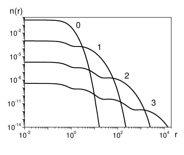
Figure 4: One-particle density distributions for the ground ($n=0$) and excited ($n=1,2,3$) states.

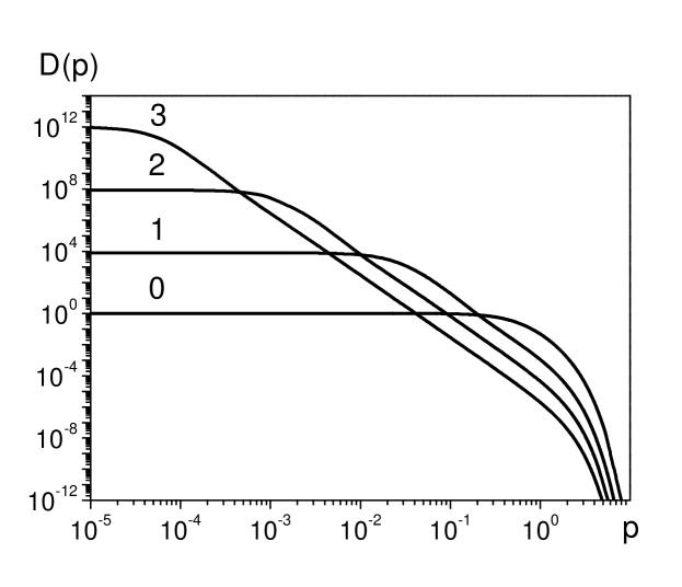
Figure 8: Momentum distributions for the ground ($n=0$) and three excited ($n=1,2,3$) states.

References

- (1) V. N. Efimov, Yad. Fiz. 12, 1080 (1970) (in Russian).
- (2) V. N. Efimov, Yad. Fiz. 29, 1058 (1979) (in Russian).
- (3) V. Efimov, Nucl. Phys. A362, 45 (1981).
- (4) R. A. Minlos, L. D. Faddeev, Zh. Eksp. Teor. Fiz. 41, 1850 (1961) (in Russian).
- (5) I. V. Simenog, D. V. Shapoval, Yad. Fiz. 47, 971 (1988) (in Russian).
- (6) I. V. Simenog, D. V. Shapoval, Teor. Mat. Fiz. 75, 275 (1988) (in Russian).
- (7) I. V. Simenog, A. I. Sitnichenko, Dopovidi AN UkrSSR, Ser. fiz. , 11, 74 (1981) (in Ukrainian).
- (8) A. C. Antunes, V. I. Baltar and E. M. Ferreira, Nucl. Phys. A265, 365 (1976).
- (9) I. V. Simenog, A. I. Sitnichenko, Ukr. Phys. J. 28, 1 (1983) (in Russian).
- (10) V. I. Kukulin, V. M. Krasnopol’sky, J.Phys. G: Nucl.Phys. 3, 795 (1977).
- (11) K. Varga, Y. Suzuki, Phys. Rev. C. 52, 2885 (1995).
- (12) I. V. Simenog, S. M. Bubin, J. of Physical. Studies. 4, 124 (2000) (in Ukrainian).
- (13) B. E. Grinyuk, I. V. Simenog, Ukr. Phys. J. 45, 625 (2000) (in Ukrainian).
- (14) I. V. Simenog, I. S. Dotsenko, B. E. Grinyuk, Ukr. Phys. J. 47, 129 (2002).
- (15) E. Nielsen, D. V. Fedorov, A. S. Jensen and E. Garrido, Phys. Reports. 347, 373 (2001).
- (16) Yu. V. Orlov, V. V. Turovtsev, Zh. Eksp. Teor. Fiz. 86, 1600 (1984) (in Russian).