Abstract

The formalism of two coupled Dirac equations within constraint instant form dynamics is used to study the nucleon-nucleon (NN) interaction. The salient features and the final Schrödinger type equation is given. Explicitly energy dependent coupled channel potentials, for use in partial wave Schrödinger like equations, with nonlinear and complicated derivative terms, result. We developed the necessary numerics and study $np$ and $pp$ scattering phase shifts for energies 0–3 GeV and the deuteron bound state. The interactions are inspired by meson exchange of $\pi,\eta,\rho,\omega$ and $\sigma$ mesons for which we adjust coupling constants. This yields, in the first instant, high quality fits to the Arndt phase shifts 0–300 MeV. Second, the potentials show a universal, independent from angular momentum, core potential which is generated from the relativistic meson exchange dynamics. Extrapolations towards higher energies, up to $T_{Lab}=3$ GeV, allow to separate a QCD dominated short range zone as well as inelastic nucleon excitation mechanism contributing to meson production. A local and/or nonlocal optical model, in addition to the meson exchange Dirac potential, produces agreement between theoretical and data phase shifts. Third, the ${}^{1}S_{0},\ ^{3}P_{0}$ and ${}^{3}P_{1}$ partial waves elicit a fusion/scission, for $T_{Lab}<1$ GeV, and a fusion/fission, for $T_{Lab}>1$ GeV, mechanism for intermediate dibaryon formation.

1 Introduction

The formalism of coupled two-body Dirac equations, within constraint instant form dynamics, is used to study the nucleon-nucleon (NN) interaction. This particular approach for two spin 1/2 particles was developed by Crater, Van Alstine, Long and Liu [2, 3, 7, 4, 5, 6]. They define a Poincaré invariant interaction in terms of scalar, pseudo scalar, vector etc. interactions with the implication that they satisfy certain compatibility conditions [7]. This approach yields in its final form explicitly energy dependent coupled channel potentials for use in partial wave Schrödinger like equations [5]. We followed and re-derived their expressions up to a certain point and developed our own numerics to study $np$ and $pp$ scattering phase shifts for $0<T_{Lab}<3$ GeV. The comparison with recent data makes use of SM00 and SP03 GWU/VPI SAID phase shift solutions [8].

The NN interaction is described within the paradigm of exchange mechanism involving $\pi,\rho,\omega\,\sigma$ and other mesons exchanges [11] to make up what we call the Dirac potential. A comparison with most recent experimental data, GWU/VPI SP03 phase shifts, requires the adjustment of coupling constants and a regularization of the short range interaction domain. For energies above pion production threshold $280<T_{Lab}<3000$ MeV we added a phenomenological complex optical model potential to the Dirac potential. This addition brings the theoretical S-matrix in perfect agreement with the experimental data S-matrix from GWU/VPI and, more importantly, permits the identification of some predominant reaction paths.

The coupled two-body Dirac equations, combined with the meson exchange model, yield the appearance of a repulsive, practically hard core, potential independent of partial wave. The universal core radius has a value $r_{c}=0.5\pm 0.025$ fm. This core radius is independent of a nucleon substructure. It depends only on masses, in particular of the exchanged mesons, and the full relativistic treatment of the NN system. This feature is not present with equal distinctness in any of the current NN best fit potentials of np and pp data [9, 10, 11]. For purpose of comparison, we show results of the Argonne AV18 potential [10].

The fitting process of coupling constants uses data in the sub-meson-production domain, $0<T_{Lab}<280$ MeV, of np and pp partial wave phase shifts. For $T_{Lab}>280$ MeV, single and double intrinsic nucleon excitations, $\Delta(3,3)$ and other low excited hadrons, as well as simple and complex reactive meson productions contribute. This is well known and demands beyond NN a more complex coupled channels problem to solve. We curtail the problem to NN scattering using an optical model potential (OMP) addition [12, 13]. Despite of complicated inelasticities, selection rules of angular momentum, isospin selection and the complex energy dependences some of the partial waves show that the real phase shifts $\delta(T)$, are very well reproduced (extrapolated) by the Dirac potential alone. Most clearly, this is realized in the ${}^{1}S_{0}$,${}^{3}P_{0}$ and ${}^{3}P_{1}$ channels and $T_{Lab}<1100$ MeV. We have realized this fact before [12, 13] but wish now to support more convincingly the case of an intermediate fusion/scission, for $T_{Lab}<1$ GeV, and a fusion/fission, for $T_{Lab}>1$ GeV, mechanism in which two nucleons change briefly into a compact dibaryon with subsequent decay back into two nucleons and mesons.

In Fig. 1 we show an intuitive and guiding scheme which distinguishes interaction domains as function of separation between the two nucleons.

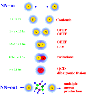
Figure 1: NN scattering and reaction scheme for $T_{Lab}<3$ GeV.

This scheme is in accordance with coupled channels.

2 Theoretical background

Relativistic quantum mechanics demands a Poincaré invariant formulation. This implies unitary representations of the Poincaré group as transformations for state vectors. One distinguishes ten generators for translations and rotations

$$P_{\mu}(4)\quad\text{and}\quad J_{\mu\nu}(6)=-J_{\nu\mu}.$$ (1)

The associated commutation relations yield the Poincaré algebra. Subsets of these generators are associated with subgroups, which correspond to 3D hypersurfaces in Minkowski space. The kinematic subgroups are instant form $x^{0}=0$, light front form $x^{0}+x^{3}=0$ and point form $x\cdot x=a^{2}>0$ with $x^{0}>0$ [1]. Within the fundamental variables, one distinguishes simple kinematic variables and complex Hamiltonians.

Crater, Van Alstine and their collaborators [2, 3, 7, 6, 5] treat the nucleon-nucleon problem with two coupled Dirac equations. Each of the two free nucleons satisfies

$$(i\gamma^{\mu}\partial_{\mu}-m)\psi=0\quad\text{and}\quad(\hat{p}^{2}+m^{2})\psi=0.$$ (2)

They relate to a representation in terms of Todorov’s variables

$$x=x_{1}-x_{2}\quad\text{relative distance}$$

$$P=p_{1}+p_{2}\quad\text{total momentum}$$

$$\omega=\sqrt{-P^{2}}\quad\text{invariant mass, in C.M. total energy}$$

$$(P^{2}+\omega^{2})\Psi=0,\quad\vec{P}=0\quad\text{in C.M.}$$

$$\hat{P}_{\nu}=\frac{P_{\nu}}{\omega},\quad x_{\perp}^{\nu}=(\eta^{\nu\mu}+\hat{P}^{\nu}\hat{P}^{\mu})x_{\mu}\quad\text{transverse coordinate}$$

$$\epsilon_{1}=\frac{\omega^{2}+m_{1}^{2}-m_{2}^{2}}{2\omega},\quad\epsilon_{2}=\frac{\omega^{2}+m_{2}^{2}-m_{1}^{2}}{2\omega}$$

$$m_{\omega}=\frac{m_{1}\,m_{2}}{\omega}\ \text{relativistic reduced mass}$$

$$\epsilon_{\omega}=\frac{\omega^{2}-m_{1}^{2}-m_{2}^{2}}{2\omega}\quad\text{relativistic relative energy on reduced mass}$$

$$p=\frac{\epsilon_{2}p_{1}-\epsilon_{1}p_{2}}{\omega},\quad P\cdot p=0,\quad p_{1}=\frac{\epsilon_{1}P}{\omega}+p,\quad p_{2}=\frac{\epsilon_{2}P}{\omega}-p$$

$$k^{2}=p^{2}=b^{2}(\omega,m_{1},m_{2})=\frac{\omega^{4}+(m_{1}^{2}-m_{2}^{2})^{2}-2\omega^{2}(m_{1}^{2}+m_{2}^{2})}{4\omega^{2}}$$

$$=\epsilon^{2}_{\omega}-m_{\omega}^{2}=\epsilon_{1}^{2}-m_{1}^{2}=\epsilon_{2}^{2}-m_{2}^{2}.$$

In particular $\theta$-matrices are related to $\gamma$-matrices.

$$\eta^{\mu\nu}=\eta_{\mu\nu}=\text{diag(-1,1,1,1)},\quad\theta^{\mu}=i\sqrt{\frac{1}{2}}\gamma_{5}\gamma^{\mu},\quad\theta_{5}=i\sqrt{\frac{1}{2}}\gamma_{5},$$

$$\theta_{\perp}^{\nu}=(\eta^{\nu\mu}-P^{\nu}P^{\mu}/P^{2})\theta_{\mu}$$

Several anticommutator relations hold, viz.

$$[\theta^{\mu},\theta^{\nu}]_{+}=-\eta^{\mu\nu},\quad[\theta_{5},\theta_{5}]_{+}=-1,$$

$$[\theta_{5},\theta^{\mu}]_{+}=0,\quad[\theta_{i}\cdot\hat{P},\theta_{i}\cdot\hat{P}]_{+}=1,\quad[\theta_{i}\cdot\hat{P},\theta_{\perp\,i}^{\mu}]_{+}=0.$$

The free equations are

$$(p\cdot\theta+m\theta_{5})\,\psi=0\quad\text{and}\quad(p^{2}+m^{2})\psi=0.$$ (3)

The generators of the Lorentz group $J_{\mu\nu}$ contain angular momentum and spin

$$J_{\mu\nu}=L_{\mu\nu}+S_{\mu\nu}$$

$$L_{\mu\nu}=\frac{1}{2}(q_{\mu}p_{\nu}+p_{\nu}q_{\mu}-q_{\nu}p_{\mu}-p_{\mu}q_{\nu})$$

$$S_{\mu\nu}=-\frac{i}{2}(\theta_{\mu}\theta_{\nu}-\theta_{\nu}\theta_{\mu})=\frac{i}{4}(\gamma_{\mu}\gamma_{\nu}-\gamma_{\nu}\gamma_{\mu}).$$

Each nucleon moves in the field of the other nucleon. Ultimately, the interaction is described by a meson exchange model.

For two particles with spin

$${\cal S}_{i0}=p_{i}\theta_{i}+m_{i}\theta_{5i},\quad i=1,2$$

the commutator

$$[{\cal S}_{10},{\cal S}_{20}]=0$$

vanishes strongly.

2.1 Example with scalar interaction

A scalar interaction changes the mass into a mass operator $M_{i}=m_{i}+S$. The Dirac equations are

$${\mathcal{S}}_{1}\psi=(+p\cdot\theta_{1}+\epsilon_{1}\hat{P}\cdot\theta_{1}+M_{1}\theta_{51})\psi=0$$

$${\mathcal{S}}_{2}\psi=(-p\cdot\theta_{2}+\epsilon_{2}\hat{P}\cdot\theta_{2}+M_{2}\theta_{52})\psi=0$$

$$[\mathcal{S}_{1},\mathcal{S}_{2}]\_\,\psi=-i\,(\partial M_{1}\cdot\theta_{1}\theta_{52}+\partial M_{2}\cdot\theta_{2}\theta_{51})\psi\neq 0.$$

The commutator does not vanish in general but vanishes through a third law condition

$$\partial(M_{1}^{2}(x_{\perp})-M_{2}^{2}(x_{\perp}))=0\quad\text{and}\quad M_{1}^{2}(x_{\perp})-M_{2}^{2}(x_{\perp})=m_{1}^{2}-m_{2}^{2}.$$ (4)

Using a hyperbolic parameterization

$$M_{1}=m_{1}\cosh L+m_{2}\sinh L$$

$$M_{2}=m_{2}\cosh L+m_{1}\sinh L$$

gives, in terms of a single invariant function $L=L(x_{\perp})$, a compatible representation of the scalar interaction. The two body Dirac equations, with a scalar interaction, are

$$\mathcal{S}_{1}\psi=\left(+\theta_{1}\cdot p+\epsilon_{1}\theta_{1}\cdot\hat{P}+M_{1}\theta_{51}-i\partial L\cdot\theta_{2}\theta_{52}\theta_{51}\right)\psi=0$$

$$\mathcal{S}_{2}\psi=\left(-\theta_{2}\cdot p+\epsilon_{2}\theta_{2}\cdot\hat{P}+M_{2}\theta_{52}+i\partial L\cdot\theta_{1}\theta_{51}\theta_{52}\right)\psi=0$$

$$\text{where}\quad\quad\partial L=\frac{\partial M_{1}}{M_{2}}=\frac{\partial M_{2}}{M_{1}}.$$

The Dirac constraint operators satisfy

$$\left(\mathcal{S}_{1}^{2}-\mathcal{S}_{2}^{2}\right)\psi=-\frac{1}{2}\left(p_{1}^{2}+m_{1}^{2}-p_{2}^{2}-m_{2}^{2}\right)\psi=-P\cdot p\,\psi=0.$$ (5)

Crater, Van Alstine and collaborators generalized their hyperbolic representation to apply for any interaction being Poincaré invariant, viz.

Scalar:

$$\Delta_{L}=-L\,\theta_{51}\theta_{52}=-\frac{L}{2}\mathcal{O}_{1}\quad\text{with}\quad\mathcal{O}_{1}=-\gamma_{51}\gamma_{52}$$

Time-like Vector:

$$\Delta_{J}=J\,\hat{P}\cdot\theta_{1}\hat{P}\cdot\theta_{2}=\mathcal{O}_{2}\frac{J}{2}=\beta_{1}\beta_{2}\frac{J}{2}\mathcal{O}_{1}$$

Space-like Vector:

$$\Delta_{\mathcal{G}}=\mathcal{G}\,\theta_{1\perp}\cdot\theta_{2\perp}=\mathcal{O}_{3}\frac{\mathcal{G}}{2}=\gamma_{1\perp}\gamma_{2\perp}\frac{\mathcal{G}}{2}\mathcal{O}_{1}$$

Pseudo-scalar:

$$\Delta_{C}=\mathcal{E}_{1}\frac{C}{2}=-\gamma_{51}\gamma_{52}\mathcal{O}_{1}\frac{C}{2}$$

and four others of which we shall not make any use. With such sum of interactions

$$\Delta=\Delta_{J}+\Delta_{L}+\Delta_{\mathcal{G}}+\Delta_{C},$$ (6)

the coupled system of equations

$$\mathcal{S}_{1}\psi=\left(+G\theta_{1}\cdot p+E_{1}\theta_{1}\cdot\hat{P}+M_{1}\theta_{51}+i\frac{G}{2}\left(\theta_{2}\cdot\partial\mathcal{G}\mathcal{O}_{3}+J\mathcal{O}_{2}-L\mathcal{O}_{1}+C\mathcal{E}_{1}\right)\right)\psi=0,$$

$$\mathcal{S}_{2}\psi=\left(-G\theta_{2}\cdot p+E_{2}\theta_{2}\cdot\hat{P}+M_{2}\theta_{52}-i\frac{G}{2}\left(\theta_{1}\cdot\partial\mathcal{G}\mathcal{O}_{3}+J\mathcal{O}_{2}-L\mathcal{O}_{1}+C\mathcal{E}_{1}\right)\right)\psi=0$$

are fully defined by masses, energies and single particle quantities

$$M_{1}=m_{1}\cosh(L)+m_{2}\sinh(L)$$

$$M_{2}=m_{2}\cosh(L)+m_{1}\sinh(L)$$

$$E_{1}=\epsilon_{1}\cosh(J)+\epsilon_{2}\sinh(J)$$

$$E_{2}=\epsilon_{2}\cosh(J)+\epsilon_{1}\sinh(J)$$

$$\text{and}\quad\quad G=e^{\mathcal{G}}.$$

Finally an elaborate Pauli reduction yields coupled Schrödinger type equations. $\sigma,\,\rho,\,\omega,\,\pi$ and $\eta$ exchanges specify the interactions

$$L(x_{\perp}),J(x_{\perp}),C(x_{\perp}),\mathcal{G}(x_{\perp}).$$ (7)

We use

$$\mathcal{D}=E_{1}M_{2}+E_{2}M_{1}$$ (8)

and

$$\mathcal{B}^{2}=E_{1}^{2}-M_{1}^{2}=E_{2}^{2}-M_{2}^{2}.$$ (9)

The final stationary Schrödinger type equation

$$\left\{\mathbf{p}^{2}-i\left[2\mathcal{G}^{\prime}-\frac{E_{2}M_{2}+M_{1}E_{1}}{\mathcal{D}}(J+L)^{\prime}\right]({\mathbf{\hat{r}}}\cdot\mathbf{p})\right.$$

$$-\frac{i(J-L)^{\prime}}{2}((\mathbf{\sigma}_{1}\cdot{\mathbf{\hat{r}}})(\mathbf{\sigma}_{2}\cdot\mathbf{p})+(\mathbf{\sigma}_{2}\cdot{\mathbf{\hat{r}}})(\mathbf{\sigma}_{1}\cdot\mathbf{p}))$$

$$-\frac{1}{2}\nabla^{2}\mathcal{G-}\frac{1}{4}\mathcal{G}^{\prime 2}-\frac{1}{4}(C+J-L)^{\prime}(-C+J-L)^{\prime}+\frac{1}{2}\frac{E_{2}M_{2}+M_{1}E_{1}}{\mathcal{D}}\mathcal{G}^{\prime}(J+L)^{\prime}$$

$$+(\mathbf{\sigma}_{1}\cdot\mathbf{\sigma}_{2})\left[\frac{1}{2}\nabla^{2}\mathcal{G+}\frac{1}{2}\mathcal{G}^{\prime 2}-\frac{1}{2}\frac{E_{2}M_{2}+M_{1}E_{1}}{\mathcal{D}}\mathcal{G}^{\prime}(J+L)^{\prime}-\frac{1}{2}\mathcal{G}^{\prime}C^{\prime}-\frac{1}{2}\frac{\mathcal{G}^{\prime}}{r}-\frac{1}{2}\frac{(-C+J-L)^{\prime}}{r}\right]$$

$$+\frac{\mathbf{L}\cdot(\mathbf{\sigma}_{1}+\mathbf{\sigma}_{2})}{r}\left[\mathcal{G}^{\prime}-\frac{1}{2}\frac{E_{2}M_{2}+M_{1}E_{1}}{\mathcal{D}}(J+L)^{\prime}\right]$$

$$-\frac{\mathbf{L}\cdot(\mathbf{\sigma}_{1}-\mathbf{\sigma}_{2})}{r}\frac{1}{2}\frac{E_{2}M_{2}-M_{1}E_{1}}{\mathcal{D}}(J+L)^{\prime}$$

$$+\frac{\mathbf{L}\cdot(\mathbf{\sigma}_{1}\times\mathbf{\sigma}_{2})}{r}\frac{i}{2}\frac{M_{2}E_{1}-M_{1}E_{2}}{\mathcal{D}}(J+L)^{\prime}$$

$$+(\mathbf{\sigma}_{1}\cdot{\mathbf{\hat{r}}})(\mathbf{\sigma}_{2}\cdot{\mathbf{\hat{r}}})\left[-\frac{1}{2}\nabla^{2}(-C+J-L)-\frac{1}{2}\nabla^{2}\mathcal{G-G}^{\prime}(-C+J-L)^{\prime}-\mathcal{G}^{\prime 2}+\frac{3}{2r}\mathcal{G}^{\prime}\right.$$

$$\left.\left.+\frac{3}{2r}(-C+J-L)^{\prime}+\frac{1}{2}\frac{E_{2}M_{2}+M_{1}E_{1}}{\mathcal{D}}(J+L)^{\prime}(\mathcal{G}-C+J-L)^{\prime}\right]\right\}|\phi_{+}\rangle$$

$$=e^{-2\mathcal{G}}\mathcal{B}^{2}|\phi_{+}\rangle$$ (10)

can be treated with well known techniques, in particular partial wave expansion, to find angular momentum (with spin, isospin and angular momentum) dependent radial Schrödinger equations.

3 Dirac Potentials and Partial Wave Phase Shifts

Partial wave expansion separates spin, angular and radial parts to yield coupled or uncoupled radial Schrödinger type equations

$$-\phi^{\prime\prime}(r,k)+V_{1}(r)\phi^{\prime}(r,k)+V_{0}(r)\phi(r,k)=k^{2}\phi(r,k).$$ (11)

The appearance of a first derivative term requires solving a system of first order equations which is numerically not favorable. However, the Numerov algorithm is favorable and popular for radial Schrödinger equations but applies only to second order, without first derivative, equations. A factorization of the solution $\phi(r,k)$ by the ansatz

$$\phi(r,k):=g(r,k)f(r,k)$$

yields first order equations

$$g^{\prime}(r,k)=\frac{1}{2}V_{1}(r)g(r,k)\quad\text{with}\quad\lim_{r\to\infty}g(r,k)=1$$ (12)

or second order equations

$$g^{\prime\prime}(r,k)=\left(\frac{1}{2}V_{1}^{\prime}(r)+\frac{1}{4}V_{1}^{2}(r)\right)g(r,k)\quad\text{with}\quad\lim_{r\to\infty}g(r,k)=1.$$ (13)

The other factor satifies the second order equation

$$-f^{\prime\prime}(r,k)+V(r)f(r,k)=k^{2}f(r,k),\quad\lim_{r\to\infty}f(r,k)\sim\frac{1}{2i}(-h^{-}(r,k,\eta)+h^{+}(r,k,\eta)\,S(k)).$$ (14)

Ricatti Hankel or Coulomb functions $h^{\pm}(r,k,\eta)$ and the S-matrix $S(k)$ determine the asymptotic solutions. We identify the Dirac potential with

$$V^{D}(r)=g^{-1}(r,k)\left(\frac{1}{4}V_{1}^{2}(r)-\frac{1}{2}V_{1}^{\prime}(r)+V_{0}(r)\right)g(r,k)$$ (15)

and additionally centrifugal and Coulomb potentials

$$V^{FC}(r)=g^{-1}(r,k)\left(\frac{\ell(\ell+1)}{r^{2}}+\frac{2k\,\eta(k)}{r}\right)g(r,k).$$ (16)

We use the convention of [7, 5]

$$P=p_{1}+p_{2}\quad\text{total momentum},$$

$$\omega=\sqrt{-P^{2}}\quad\text{invariant mass, in C.M. total energy,}\quad\vec{P}=0\quad\text{in C.M.},$$

$$\epsilon_{1}=\frac{\omega^{2}+m_{1}^{2}-m_{2}^{2}}{2\omega},\quad\epsilon_{2}=\frac{\omega^{2}+m_{2}^{2}-m_{1}^{2}}{2\omega},$$

$$m_{\omega}=\frac{m_{1}\,m_{2}}{\omega}\quad\text{relativistic reduced mass},$$

$$\epsilon_{\omega}=\frac{\omega^{2}-m_{1}^{2}-m_{2}^{2}}{2\omega}\quad\text{relativistic relative energy,}$$

$$p=\frac{\epsilon_{2}p_{1}-\epsilon_{1}p_{2}}{\omega},\quad p_{1}=\frac{\epsilon_{1}P}{\omega}+p,\quad p_{2}=\frac{\epsilon_{2}P}{\omega}-p,$$

$$k^{2}=p^{2}=\frac{\omega^{4}+(m_{1}^{2}-m_{2}^{2})^{2}-2\omega^{2}(m_{1}^{2}+m_{2}^{2})}{4\omega^{2}}=\epsilon^{2}_{\omega}-m_{\omega}^{2}=\epsilon_{1}^{2}-m_{1}^{2}=\epsilon_{2}^{2}-m_{2}^{2},$$

$$\eta(k)=\frac{\epsilon_{\omega}\,e^{2}}{k}\delta_{pp}\quad\text{Coulomb parameter.}$$

This is to be compared with standard non-relativistic NN potentials [10]. The recent work by Liu and Crater [5] elaborates on other methods to determine phase shifts from Eq. (11).

The model specification for $L(x_{\perp}),J(x_{\perp}),C(x_{\perp})$ and ${\mathcal{G}}(x_{\perp})$ follows Liu and Crater model I [5] to specify scalar

$$S=-g^{2}_{\sigma}\frac{e^{-m_{\sigma}r}}{r}-(\tau_{1}\cdot\tau_{2})g^{2}_{a_{0}}\frac{e^{-m_{a_{0}}r}}{r}-g^{2}_{f_{0}}\frac{e^{-m_{f_{0}}r}}{r},$$

pseudo scalar

$$C=(\tau_{1}\cdot\tau_{2})\frac{g^{2}_{\pi}}{\omega}\frac{e^{-m_{\pi}r}}{r}+\frac{g^{2}_{\eta}}{\omega}\frac{e^{-m_{\eta}r}}{r}-\frac{g^{2}_{\eta^{\prime}}}{\omega}\frac{e^{-m_{\eta^{\prime}}r}}{r},$$

and vector

$$A=(\tau_{1}\cdot\tau_{2})g^{2}_{\rho}\frac{e^{-m_{\rho}r}}{r}+g^{2}_{\omega}\frac{e^{-m_{\omega}r}}{r}+g^{2}_{\phi}\frac{e^{-m_{\phi}r}}{r}$$

interactions. All Yukawa form factors are regularized with a normalized Gaussian

$$\frac{e^{-m\,r}}{r}\to N_{G}(a)\int dx^{3}\,\frac{e^{-m\,x}}{x}\,e^{-(\vec{r}-\vec{x})^{2}/a^{2}}\quad\text{with}\quad a=0.14142\,\text{fm.}$$ (17)

For $S<0$ we use

$$\sinh(L)=\frac{S\,G^{2}}{w}\left(1+\frac{G^{2}(\epsilon_{\omega}-A)S}{m_{\omega}\sqrt{\omega^{2}+S^{2}}}\right),$$ (18)

and for $S>0$

$$M_{1}^{2}=m_{1}^{2}+G^{2}(2m_{w}S+S^{2})$$

$$M_{2}^{2}=m_{2}^{2}+G^{2}(2m_{w}S+S^{2})$$

$$\partial L=\frac{\partial M_{1}}{M_{2}}=\frac{\partial M_{2}}{M_{1}}.$$

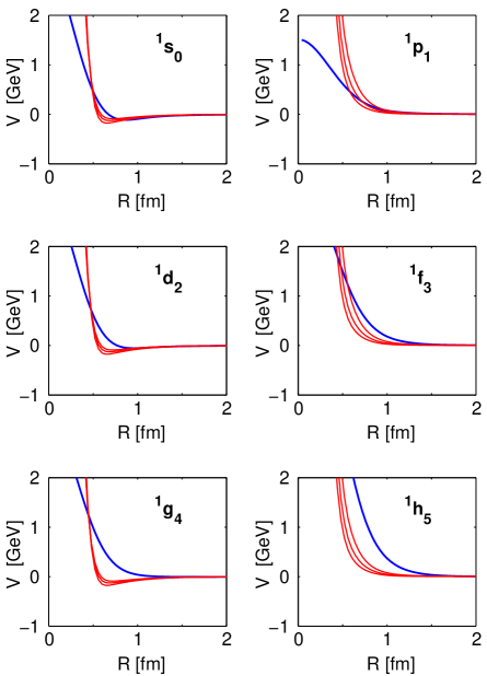
Figure 3: Dirac potentials (red) for singlet $S=0$, $T=0$ (right column) and $T=1$ (left column) channels. Differences between $np$ and $pp$ potentials are very small. The Coulomb potential is added for pp. The AV18 channel potential is shown as blue line.

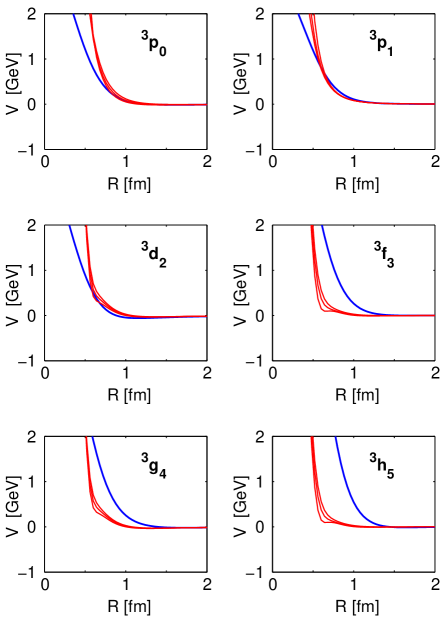
Figure 4: Dirac potentials (red) for triplet $S=1$, $T=0,1$ uncoupled channels. The AV18 channel potential is shown as blue line.

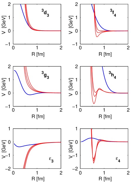
Figure 6: Dirac potentials (red) for triplet $S=1$, $T=0,1$ coupled channels. The AV18 channel potential is shown as blue line.

This models $\pi,\,\eta,\,\rho,\,\omega,\,\delta$ and $\sigma$ exchanges. In Figs. 3, 4, 5 and 6 are shown Dirac potentials for three values, $T_{Lab}=[0.1,1,2]$ GeV (red lines). In comparison are shown the results of the popular Argonne AV18 potential (blue line) [10]. The remarkable feature of the Dirac potentials is their universal repulsive core with $r_{c}\sim 0.5$ fm. The only exception is the ${}^{3}PF_{1}$ channel where the ansatz of repulsion turns, surprisingly, into a short range attraction.

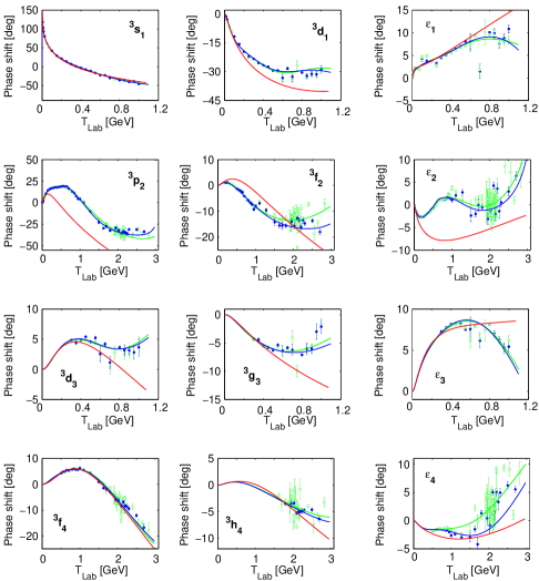
Figure 8: Coupled channels $pp$ [0,3] GeV, $np$ [0,1.2] GeV SM00 and SP03 real phase shift data $\delta(T)$ and theoretical curve based soly upon Dirac potential (red line). The full potential, Dirac and OMP, describes the data SP03. SM00 (continuous solution, green, single energy solutions, open green circles, with error bars) and SP03 (continuous solutio, blue, single energy solutions, full blue circles, with error bars) and theoretical results (real Dirac potential solutions, red line, real Dirac potentials with complex OMP added are coinciding with the data of SP03 blue line).

In Figs. 7 and 8 are shown the phase shifts of SM00 (green), SP03 (blue) and theoretical results (real Dirac potential solutions (red), real Dirac potentials with complex OMP added are coinciding with the data of SP03 blue lines).

The Dirac instant form dynamic yields partial wave spin, isospin and energy ($\alpha$ channel) dependent NN potentials $V_{\alpha}^{D}(r,T)$ to which we add a local or nonlocal optical model potential whose strengths are fitted to data

$$V(r)=V_{\alpha}^{D}(r,T)+[U_{\alpha}(T)g(r)+iW_{\alpha}(T)g(r)]$$ (19)

or

$$V(r,r^{\prime})=V_{\alpha}^{D}(r,T)\delta(r-r^{\prime})+|\phi(r)>[U_{\alpha}(T)+iW_{\alpha}(T)]<\phi(r^{\prime})|.$$ (20)

Since local/nonlocal potentials imply similar results, we restrict ourselves here to the local optical potential and reference the more general and nonlocal case [12].

A remark about phase shift convention appears necessary. Consider the partial wave radial equation

$$-f^{\prime\prime}_{\alpha}(r,k)+V_{\alpha}(r)f_{\alpha}(r,k)=k^{2}f_{\alpha}(r,k)$$ (21)

with stationary

$$f^{0}\sim j(kr)+n(kr)\,K(k)$$ (22)

or physical boundary conditions

$$\quad f^{+}\sim\frac{1}{2i}(-h^{-}(kr)+h^{+}(kr)\,S(k)).$$ (23)

$S$- and $K$-matrices are related to phase shifts [14]. There exist several conventions to represent the S-matrix in terms of phase shifts. The Arndt and Roper [14] (GWU/VPI) convention uses S- and K-matrices

$$S=(1+iK)(1-iK)^{-1},\quad\text{with}\quad K=i(1-S)(1+S)^{-1}=\text{Re}\,K+i\,\text{Im}\,K.$$ (24)

$\text{Re}\,K$ corresponds to a unitary S-matrix and phase shifts $\delta^{\pm}(k)$ and $\varepsilon(k)$ defined by

$$S(\text{Re\,}K)=\begin{pmatrix}\cos(2\varepsilon)\exp(2i\delta^{-})&i\sin(2\varepsilon)\exp(i(\delta^{-}+\delta^{+}))\\ i\sin(2\varepsilon)\exp(i(\delta^{-}+\delta^{+}))&\cos(2\varepsilon)\exp(2i\delta^{-})\end{pmatrix}.$$ (25)

Absorption phase shifts, $\rho^{\pm}$ and $\mu$, are related to

$$\text{Im\,}K=\begin{pmatrix}\tan^{2}\rho^{-}&\tan\rho^{-}\tan\rho^{+}\cos\mu\\ \tan\rho^{-}\tan\rho^{+}\cos\mu&\tan^{2}\rho^{+}\end{pmatrix}.$$ (26)

Single channels simplify to $K=\tan\delta+i\tan^{2}\rho$.

4 The Nucleon-Nucleon Optical Potential

The notion of an optical model is useful in cases when the S-matrix is not unitary and flux disappears into open inelastic or reaction channels. The optical model is often expressed in terms of a complex and energy dependent potential where the imaginary part effectively describes the loss of flux without specification of the inelastic channels. A less popular alternative to a complex optical model potential is the introduction of pseudo channels. Here we follow the optical potential approach [12].

The source of the BB channel (dibaryon formation) is the NN core-domain whose transition is mediated by a delta-function or a narrow Gaussian function. Intrinsic nucleon excitations are also mediated by a narrow Gaussian in the core domain. Inelasticities are either generated by coupling BB (dibaryon) to asymptotic many body final states, composed of two nucleons and mesons, or decay of XY, composed of one or two intrinsic nucleon excitations, into asymptotic many body final states. Within the inner core region $r<r_{c}$ NN and XY wave function components vanish. The meson exchange Dirac potential, which is described by the NN Dirac instant form dynamics, should ultimately be limited to $r\geq r_{c}\sim 0.5\,\text{fm}$ in its effect. This constraint eliminates the need for regularization of the short range Dirac potential and boundary conditions are automatically generated by the $\delta(r-r_{c})$ $NN\leftrightarrow BB$ transition potentials. This proposal is demonstrated in Fig. 2. The strengths and location of $\delta$-function interactions are boundary conditions which are to be determined by BB and XY models. Herein lies the essential point of our method. Dirac potentials play only the role of a shield which prevents us from seeing the naked refinement surface of hadronic QCD dynamics – it recalls the P-matrix formalism. A realization of the full coupled channels problem is in progress.

Without specification of details, the coupling scheme has the following structure

$$\mathcal{H}_{BB}\ + \mathcal{V}_{BB}^{NN}\delta(r-r_{c}) +\ \mathcal{V}_{BB}\quad\quad\text{confined dibaryon, NN meson decay}$$

$$\Big{\updownarrow}$$

$$\mathcal{V}_{NN}^{BB}\delta(r-r_{c}) +\ \mathcal{V}_{NN}^{XY}g(r-r_{c})+H_{NN}+V_{NN}^{\text{\tiny Dirac}}\quad\quad\text{NN elastic}$$ (29)

$$\quad\quad\Big{\updownarrow}$$

$$\ \mathcal{V}_{XY}^{NN}g(r-r_{c})+\mathcal{H}_{XY}+\mathcal{V}_{XY}\quad\quad\text{NN meson decay}.$$

Below pion production threshold, $T_{Lab}\sim 280$ MeV, the NN S-matrix is unitary for all practical purposes. Above this energy excitation of $\Delta$(3,3) resonances is the predominant mechanism. It is obviously present in the NN ${}^{1}D_{2},\ ^{3}F_{3}$ and ${}^{3}PF_{2}$ channels. Isospin conservation suppresses a coupling to N$\Delta$ in the $np$ $T=0$ channels.

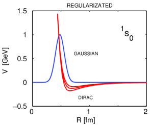
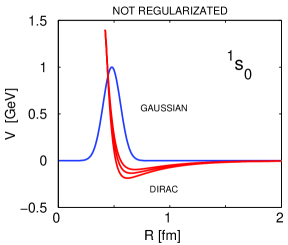
Figure 2: Dirac potential (red), left figure regularized and right figure not regularized, for the np ${}^{1}S_{0}$ channel, $T_{Lab}$ 0.1, 1 and 2 GeV, showing a long range OPEP tail, an attractive pocket $\sim 0.75$ fm and a core repulsion with $r_{c}=0.5\pm 0.025$ fm (blue). The regularized and not-regularized potentials show, in all channels, only small differences. Regularization does not affect the conclusion drawn about the core geometry generated but helps to keep numbers reasonable near the origins. Also inserted are Gaussian form factors $g(r-r_{0})\sim\exp(-(r-r_{0})^{2}/a^{2})$ which are used with the optical model (thin line curve). In this figure $r_{0}=r_{c}=0.5$ fm and $a=0.2$ fm.

NN scattering, for energies below 3 GeV in general, show a comparable to nucleon-nucleus scattering weak and smoothly energy dependent coupling to inelastic channels. A perturbative treatment of inelastic and reaction channels with DWBA methods is thus strongly favored.

A key issue for all secondary applications of NN scattering is a high quality reproduction of the elastic NN scattering channel. Inverse scattering methods are useful for this purpose. These methods use the experimental data in form of partial wave phase shifts as input and determine the optical model potential as a correction to a theoretically defined and numerically realized reference potential.

Figure 5: Dirac potentials (red) for triplet $S=1$, $T=0,1$ coupled channels. The AV18 channel potential is shown as blue line.

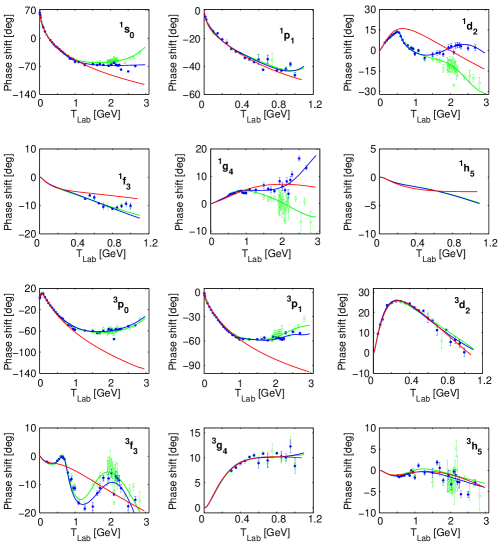
Figure 7: Single channel, $pp$ [0,3] GeV, $np$ [0,1.2] GeV SM00 (green) and SP03 (blue) real phase shift data $\delta(T)$ and theoretical curve based soly upon Dirac potential (red). The full potential, Dirac and OMP, describes the data SP03. Of particular interest are ${}^{1}S_{0},^{3}P_{0},^{3}P_{1}$ channels in which the real phase shift of the Dirac potentials coincide with data for [0,1.1] GeV but diverge above 1.1 GeV. Obvious are effects due to $\Delta(3,3)$ coupling in other channels. SM00 (continuous solution (green), single energy solutions, open green circles, with error bars). SP03 (continuous solution (blue), single energy solutions,full blue circles, with error bars). Theoretical results (real Dirac potential solutions, full red line, real Dirac potentials with complex OMP added are coinciding with the data of SP03 blue line).

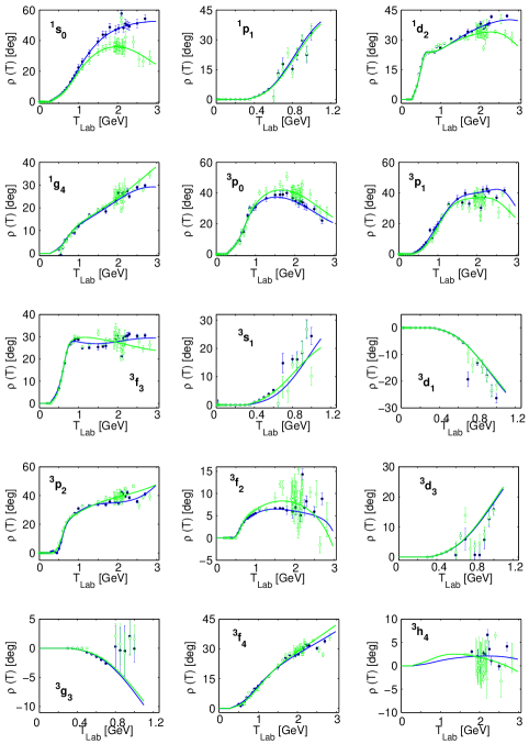
Figure 9: Available absorption phase shifts $\rho(T)$. Dirac potentials generate no absorption and OMP parameters $U_{G}(T)$ and $W_{G}(T)$ are adjusted to reproduce the continuous energy solutions of $\rho(T)$. SM00 (continuous solution, green, single energy solutions, open green circles, with error bars) and SP03 (continuous solution, blue, single energy solutions, full blue circles, with error bars) and theoretical results (real Dirac potential solutions, red, real Dirac potentials yields no absorption but with a complex OMP added the results are coinciding with the data of SP03 blue line).

4.1 ${}^{1}S_{0},\ ^{3}P_{0}$ and ${}^{3}P_{1}$ Channels

NN phase shift data, see Figs. 7 and 9, show in almost all channels and for $T_{Lab}>280$ MeV a complicated energy dependence and deviations from the Dirac potential predictions. Exceptional cases are the ${}^{1}S_{0},\ ^{3}P_{0}$ and ${}^{3}P_{1}$ channels, contained in Fig. 7, which show a practical perfect reproduction

$$\delta_{Data}=\delta_{Dirac},\quad\mbox{for}\quad 0<T_{Lab}<1100\,\text{MeV}$$ (30)

by the Dirac potential alone. However, the absorption

$$\rho_{Data}\neq 0,\quad\mbox{whereas}\quad\rho_{Dirac}=0\quad\mbox{for}\quad 280<T_{Lab}<1100\,\text{MeV.}$$ (31)

This demands an optical potential $U(r)+iW(r)$ that leaves the real phase shifts $\delta(k)$ unchanged but generates an absorption $\rho(T)>0$ for $280<T_{Lab}<1100$ MeV.

The optical potential solutions are complex

$$-f_{r}^{\prime\prime}+(V^{D}+U)f_{r}-k^{2}f_{r}=+Wf_{i}$$

$$-f_{i}^{\prime\prime}+(V^{D}+U)f_{i}-k^{2}f_{i}=-Wf_{r}$$

and the boundary conditions, $\delta=\delta(V^{D},U,W)$ and $\rho=\rho(V^{D},U,W)$, are transcendental functions of potentials and OMP adjustable parameters.

A sensible solution is $U(r)=0$ and $W(r)=W\delta(r-r_{0})$ as optical model interaction in Eq. (19). We used a delta-function and/or a narrow normalized Gaussian, see Fig. 2,

$$W(r)=\begin{cases}W_{G}\,N(r_{0},a_{0})\exp(-(r-r_{0})^{2}/a_{0}^{2})\\ W_{\delta}\,\delta(r-r_{0})\end{cases}$$ (32)

with $U=0$, starting at the origin with

$$f_{r}(0)=0,\ f_{r}(h)=h^{(\ell+1)},\ f_{i}(r)=0\quad\mbox{for}\quad 0\leq r\leq r_{0}.$$ (33)

The following conclusions are drawn: The phase-shifts $\delta(T),\,\rho(T)$ for $280<T_{Lab}<1100$ MeV imply an optical potential at the surface of the repulsive core for ${}^{1}S_{0},\,^{3}P_{0}$ and ${}^{3}P_{1}$ partial waves. Intermediate dibaryons are practically not formed, the BB channel is realized by a dibaryon fusion/scission picture as shown in Fig. 11. The BB dibaryon quark dynamic is reduced to energy dependent complex boundary conditions at the core radius permitting meson production. The meson exchange mechanism is not valid inside the core radius. Caveat, at this stage of our work, we integrated from the origin through the core region realizing a small real wave function at the core radius. This, in connection with the Gaussian OMP form factor, causes a real and imaginary part OMP $U_{G}(T)\neq 0$ and $W_{G}(T)\neq 0$.

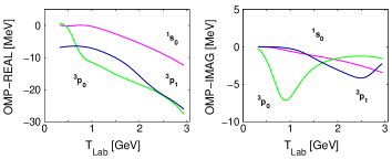
Figure 10: Selected set of optical model strengths values $U_{G}(T)$ and $W_{G}(T)$.

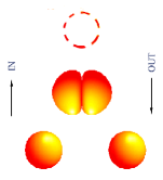
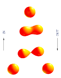
Figure 11: Left, caused by the Pauli exclusion principle for a six-quark dibaryon and $T_{Lab,NN}<1100$ MeV suggests a futile ringing of the nucleons and a suppression of dibaryon formation. It gives the impression of a fusion/scission mechanism. Right, the formation of dibaryons, at sufficient high energy, is governed by medium to longer ranged quark-gluon flux tubes with fusion into a six-quark hadron sized dibaryon with sequential decay. This inspires a fusion/fission mechanism.

In Fig. 10 are shown the np OMP (normalized Gaussian, $r_{0}=r_{c}=0.5$ fm and $a_{0}=0.2$ fm) strengths values. The crucial center of baryon $NN$ and $BB$ transition radius is $r_{0}=0.5\pm 0.025$ fm. At higher energies $T_{Lab}>1.1$ GeV, the transition surface becomes more and more faded, washed-out and translucent when the energy of dibaryon states matches the total energy of the NN system. Intermediate short lived dibaryons $J_{BB}^{P}=0^{+},\ 0^{-},\ 1^{1}$ are formed, see Fig. 11.
We estimate, from the phase behavior in these three channels, the total energy (lowest mass) of a dibaryon system $m_{BB}=2400\pm 150$ MeV and a width $\Gamma>150$ MeV.
Coupling to dibaryons is realized for $T_{Lab}>1100$ MeV and the fusion/scission picture may change gradually into a fusion/fission picture as shown in Fig. 11.

References

[1] P. A. M. Dirac,
Rev. Mod. Phys. 21, 392 (1949);
Can. J. Math. 2, 129 (1950);
Proc. Roy. Soc. Sect. A 246, 326 (1958).
[2] H. Crater and P. Van Alstine,
Ann. Phys. (NY) 148, 57 (1983).
[3] H. Crater and P. Van Alstine, Phys. Rev. D 36, 3007 (1987).
[4] H. Crater and P. Van Alstine, Relativistic Calculation of the Meson Spectrum: a Fully Covariant
Treatment Versus Standard Treatments, arXiv:hep-ph/0208186.
[5] B. Liu and H. Crater, Phys. Rev. C 67, 024001 (2003);
arXiv:nucl-th/0208045.
[6] H. Crater, B. Liu and P. Van Alstine, arXiv:hep-ph/0306291.
[7] P. Long and H. Crater, J. Math. Phys. 39, 124 (1998).
[8] R. A. Arndt, I. I. Strakovsky and R. L. Workman,
Phys. Rev. C 62, 034005 (2000); http//gwdac.phys.gwu.edu;
ssh -l said.gwdac.phys.gwu.edu.
[9] V. G. J. Stoks, R. Timmermans and J. J. de Swart,
Phys. Rev. C 47, 512 (1993); C 48, 792 (1993); C 49, 2950 (1994).
[10] R. B. Wiringa, V. G. J. Stoks and R. Schiavilla,
Phys. Rev. C 51, 38 (1995).
[11] R. Machleidt, Phys. Rev. C 63, 024001 (2001).
[12] A. Funk, H. V. von Geramb and K. A. Amos,
Phys. Rev. C 64, 054003 (2001).
[13] H. V. von Geramb, A. Funk and H. F. Arellano,
Nucleon-Nucleon and Nucleon-Nucleus Optical Models for Energies
to 3 GeV and the Question of NN Hadronization,
arXiv:nucl-th/0105075; Proc. XX. Int. Workshop on Nuclear Theory, Rila (2001).
[14] R. A. Arndt and L. D. Roper, Phys. Rev. D 25, 97 (1982).