Abstract

Systematic analysis of ⁸B Coulomb dissociation with the Asymptotic Normalization Coefficient (ANC) method is proposed to determine the astrophysical factor $S_{17}(0)$ accurately. An important advantage of the analysis is that uncertainties of the extracted $S_{17}(0)$ coming from the use of the ANC method can quantitatively be evaluated, in contrast to previous analyses using the Virtual Photon Theory (VPT). Calculation of measured spectra in dissociation experiments is done by means of the method of Continuum-Discretized Coupled-Channels (CDCC). From the analysis of ⁵⁸Ni(⁸B,⁷Be$+p$)⁵⁸Ni at 25.8 MeV, $S_{17}(0)=22.83\pm 0.51({\rm theo})\pm 2.28({\rm expt})$ (eVb) is obtained; the ANC method turned out to work in this case within 1% of error. Preceding systematic analysis of experimental data at intermediate energies, we propose hybrid (HY) Coupled-Channels (CC) calculation of ⁸B Coulomb dissociation, which makes numerical calculation much simple, retaining its accuracy. The validity of the HY calculation is tested for ⁵⁸Ni(⁸B,⁷Be$+p$)⁵⁸Ni at 240 MeV. The ANC method combined with the HY CC calculation is shown to be a powerful technique to obtain a reliable $S_{17}(0)$.

1 Introduction

The solar neutrino problem is one of the central issues in the neutrino physics [1]. Nowadays, the neutrino oscillation is assumed to be the solution of the problem and the focus of the solar neutrino physics is to determine oscillation parameters: the mass difference among $\nu_{e}$, $\nu_{\mu}$ and $\nu_{\tau}$, and their mixing angles [2]. The astrophysical factor $S_{17}$, defined by $S_{17}(E)\equiv\sigma_{p\gamma}(E)E\exp[2\pi\eta]$ with $\sigma_{p\gamma}$ the cross section of the $p$-capture reaction ⁷Be($p,\gamma$)⁸B and $\eta$ the Sommerfeld parameter, plays an essential role in the investigation of neutrino oscillation, since the prediction value for the flux of the ⁸B neutrino, which is intensively being detected on the earth, is proportional to $S_{17}(0)$. The required accuracy from astrophysics is about 5% in errors.

Because of difficulties of direct measurements for the $p$-capture reaction at very low energies, alternative indirect measurements were proposed: $p$-transfer reactions and ⁸B Coulomb dissociation are typical examples of them. In the former the Asymptotic Normalization Coefficient (ANC) method [3] is used, carefully evaluating its validity, while in the latter the Virtual Photon Theory (VPT) is adopted to extract $S_{17}(0)$; the use of VPT requires the condition that the ⁸B is dissociated through its pure E1 transition, the validity of which is not yet clarified quantitatively.

In the present paper we propose systematic analysis of ⁸B Coulomb dissociation by means of the ANC method, instead of VPT. An important advantage of the analysis is that one can evaluate the error of $S_{17}(0)$ coming from the use of the ANC method; the fluctuation of $S_{17}(0)$, by changing the ⁸B single-particle wave functions, can be interpreted as the error of the ANC analysis [4, 5, 6, 7]. For the calculation of ⁸B dissociation cross sections, we use the method of Continuum-Discretized Coupled-Channels (CDCC) [8], which was proposed and developed by Kyushu group. CDCC is one of the most accurate methods being applicable to breakup processes of weakly-bound stable and unstable nuclei. As a subject of the present analysis, four experiments of ⁸B Coulomb dissociation done at RIKEN [9], GSI [10], MSU [11] and Notre Dame [12] are available. Among them we here take up the Notre Dame experiment at 25.8 MeV and extract $S_{17}(0)$ by the CDCC + ANC analysis, quantitatively evaluating the validity of the use of the ANC method.

It was shown in Ref. [11] that CDCC can successfully be applied to the MSU data at 44 MeV/nucleon. However, the CDCC calculation requires extremely large modelspace; typically the number of partial waves is 15,000. Thus, preceding systematic CDCC + ANC analysis of the experimental data at intermediate energies, we propose hybrid (HY) Coupled-Channels (CC) calculation by means of the standard CDCC and the Eikonal-CDCC method (E-CDCC), which allows one to make efficient and accurate analysis. E-CDCC describes the center-of-mass (c.m.) motion between the projectile and the target nucleus by a straight-line, which is only the essential difference from CDCC. As a consequence, the resultant E-CDCC equations have a first-order differential form with no huge angular momenta, hence, one can easily and safely solve them. Because of the simple straight-line approximation, results of E-CDCC may deviate from those by CDCC. One can avoid this problem, however, by constructing HY scattering amplitude from results of both CDCC and E-CDCC. This can be done rather straightforwardly, since the resultant scattering amplitude by E-CDCC has a very similar form to the quantum-mechanical one, which is one of the most important features of E-CDCC. In the latter part of the present paper we show how to perform the HY calculation and apply it to ⁵⁸Ni(⁸B,⁷Be$+p$)⁵⁸Ni at 240 MeV.

In Sec. 2 we describe the CDCC + ANC analysis for ⁵⁸Ni(⁸B,⁷Be$+p$)⁵⁸Ni at 25.8 MeV: the ANC method and CDCC are quickly reviewed in subsections 2.1 and 2.2, respectively, and numerical results and the extracted $S_{17}(0)$ are shown in subsection 2.3. In Sec. 3 the HY calculation for Coulomb dissociation, with the formalism of E-CDCC, is described (subsection 3.1) and its validity is numerically tested for ⁵⁸Ni(⁸B,⁷Be$+p$)⁵⁸Ni at 240 MeV (subsection 3.2). Finally, summary and conclusions are given in Sec. 4.

2 Systematic analysis of ⁸B Coulomb dissociation

In this section we propose CDCC + ANC analysis for ⁸B Coulomb dissociation to extract $S_{17}(0)$. First, in subsection 2.1, we give a quick review of the ANC method and discuss advantages of applying it to ⁸B Coulomb dissociation. Second, calculation of ⁸B breakup cross section by means of CDCC is briefly described in subsection 2.2. Finally, we show in subsection 2.3 numerical results for ⁵⁸Ni(⁸B,⁷Be$+p$)⁵⁸Ni at 25.8 MeV; the extracted value of $S_{17}(0)$, with its uncertainties, is given.

2.1 The Asymptotic Normalization Coefficient method

The ANC method is a powerful tool to extract $S_{17}(0)$ indirectly. The essence of the ANC method is that the cross section of the ⁷Be($p,\gamma$)⁸B at stellar energies can be determined accurately if the tail of the ⁸B wave function, described by the Whittaker function times the ANC, is well determined. The ANC can be obtained from alternative reactions where peripheral properties hold well, i.e., only the tail of the ⁸B wave function has a contribution to observables.

So far the ANC method has been successfully applied to $p$-transfer reaction such as ¹⁰Be(⁷Be,⁸B)⁹Be [4], ¹⁴N(⁷Be,⁸B)¹³C [5], and ⁷Be($d,n$)⁸B [7]. Also Trache et al. [6] showed the applicability of the ANC method to one-nucleon breakup reactions; $S_{17}(0)$ was extracted from systematic analysis of total breakup cross sections of ⁸B $\longrightarrow$ ⁷Be + $p$ on several targets at intermediate energies.

In the present paper we apply the ANC method to ⁸B Coulomb dissociation, where $S_{17}(0)$ has been extracted by using VPT based on the principle of detailed balance. In order to use VPT, the previous analyses neglected effects of nuclear interaction on the ⁸B dissociation, which is not yet well justified. Additionally, roles of the E2 component, interference with the dominant E1 part in particular, need more detailed investigation, although recently some attempts to eliminate the E2 contribution from measured spectra have been made. On the contrary, the ANC analysis proposed here is free from these problems. We here stress that as an important advantage of the present analysis, one can evaluate quantitatively the error of $S_{17}(0)$ by the fluctuation of the ANC with different ⁸B single-particle potentials.

Comparing with Ref. [6], in the present ANC analysis angular distribution and parallel-momentum distribution of the ⁷Be fragment, instead of the total breakup cross sections, are investigated, which is expected to give more accurate value of $S_{17}(0)$. Moreover, our purpose is to make systematic analysis of ⁸B dissociation at not only intermediate energies but also quite low energies. Thus, the breakup process should be described by a sophisticated reaction theory, beyond the extended Glauber model used in Ref. [6]. For that purpose, we use CDCC, which is one of the most accurate methods to be applicable to ⁸B dissociation.

2.2 The method of Continuum-Discretized Coupled-Channels

Generally CDCC describes the projectile (c) + target (A) system by a three-body model as shown in Fig. 1;

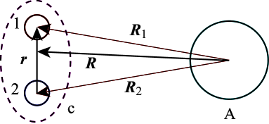
Figure 1: Schematic illustration of the system treated in the present paper.

in the present case c is ⁸B and 1 and 2 denote ⁷Be and $p$, respectively. The three-body wave function $\Psi_{JM}$, corresponding to the total angular momentum $J$ and its projection $M$, is given in terms of the internal wave functions $\varphi$ of c:

$$\Psi_{JM}=\sum_{L}{\cal Y}_{JM}^{\ell_{0}L}\varphi_{0}(r)\frac{\chi_{\ell_{0}LJ}(P_{0},R)}{R}+\sum_{\ell L}{\cal Y}_{JM}^{\ell L}\int_{0}^{\infty}\varphi_{\ell}(k,r)\frac{\chi_{\ell LJ}(P,R)}{R}dk;$$ (1)

$${\cal Y}_{JM}^{\ell L}\equiv[i^{\ell}Y_{\ell}(\Omega_{r})\otimes i^{L}Y_{L}(\Omega_{R})]_{JM},$$ (2)

where $\ell$ is the total spin of c and $L$ is the orbital angular momentum for the relative motion of c and A; the subscript 0 represents the initial state. We neglect all intrinsic spins of the constituents and as a consequence c has only one bound state in the present case. The first and second terms in the r.h.s. of Eq. (1) correspond to the bound and scattering states of c, respectively. In the latter the relative momentum $P$ between c and A is related to the internal one $k$ of c through the total-energy conservation.

In CDCC the summation over $\ell$ and integration over $k$ are truncated at certain values $\ell_{\rm max}$ and $k_{\rm max}$, respectively. For the latter, furthermore, we divide the $k$ continuum into $N$ bin-states, each of which is expressed by a discrete state $\hat{\varphi}_{i\ell}$ with $i$ denote a certain region of $k$, i.e., $k_{i-1}\leq k<k_{i}$. After truncation and discretization, $\Psi_{JM}$ is approximately expressed by $\{\hat{\varphi}_{i\ell}\}$ with finite number of channels:

$$\Psi_{JM}^{\rm CDCC}=\sum_{L}{\cal Y}_{JM}^{\ell_{0}L}\varphi_{0}(r)\frac{\chi_{\ell_{0}LJ}(P_{0},R)}{R}+\sum_{\ell=0}^{\ell_{\rm max}}\sum_{i=1}^{N}\sum_{L}{\cal Y}_{JM}^{\ell L}\hat{\varphi}_{i\ell}(r)\frac{\hat{\chi}_{\gamma}(\hat{P}_{i},R)}{R}$$ (3)

with $\gamma=\{i,\ell,L,J\}$. The $\hat{P_{i}}$ and $\hat{\chi}_{\gamma}$ are the discretized $P$ and $\chi_{\ell LJ}$, respectively, corresponding to the $i$th bin state $\hat{\varphi}_{i\ell}$.

Inserting $\Psi_{JM}^{\rm CDCC}$ into a three-body Schrödinger equation, one obtains the following (CC) equations:

$$\left[\frac{d^{2}}{dR^{2}}+\hat{P}_{i}^{2}-\frac{L(L+1)}{R^{2}}-\frac{2\mu}{\hbar^{2}}V_{\gamma\gamma}(R)\right]\hat{\chi}_{\gamma}(\hat{P}_{i},R)=\sum_{\gamma^{{}^{\prime}}\neq\gamma}\frac{2\mu}{\hbar^{2}}V_{\gamma\gamma^{{}^{\prime}}}(R)\hat{\chi}_{\gamma^{{}^{\prime}}}(\hat{P}_{i^{{}^{\prime}}},R)$$ (4)

for all $\gamma$ including the initial state, where $\mu$ is the reduced mass of the c + A system and $V_{\gamma\gamma^{\prime}}$ is the form factor defined by

$$V_{\gamma\gamma^{{}^{\prime}}}(R)=\langle{\cal Y}_{JM}^{\ell L}\hat{\varphi}_{i\ell}(r)|U|{\cal Y}_{JM}^{\ell^{{}^{\prime}}L^{{}^{\prime}}}\hat{\varphi}_{i^{{}^{\prime}}\ell^{{}^{\prime}}}(r)\rangle_{{\bf r},\Omega_{R}},$$ (5)

with $U$ the sum of the interactions between A and individual constituents of c. The CDCC equations (4) are solved with the asymptotic boundary condition:

$$\hat{\chi}_{\gamma}(\hat{P}_{i},R)\sim u_{L}^{(-)}(\hat{P}_{i},R)\delta_{\gamma,\gamma_{0}}-\sqrt{\hat{P}_{i}/\hat{P}_{0}}\hat{S}_{\gamma,\gamma_{0}}u_{L}^{(+)}(\hat{P}_{i},R),$$ (6)

where $u_{L}^{(-)}$ and $u_{L}^{(+)}$ are incoming and outgoing Coulomb wave functions. Thus one obtains the $S$-matrix elements $\hat{S}_{\gamma,\gamma_{0}}$, from which any observables, in principle, can be calculated; we followed Ref. [13] to calculate the distribution of ⁷Be fragment from ⁸B.

CDCC treats breakup chanels of a projectile explicitly, including all higher-order terms of both Coulomb and nuclear coupling-potentials, which gives very accurate description of dissociation processes in a framework of three-body reaction dynamics. Detailed formalism and theoretical foundation of CDCC can be found in Refs. [8, 14, 15].

2.3 Numerical results and the extracted $S_{17}(0)$

We here take up the ⁸B dissociation by ⁵⁸Ni at 25.8 MeV (3.2 MeV/nucleon) measured at Notre Dame [12], for which VPT was found to fail to reproduce the data [16]. The extended Glauber model, used in Ref. [6], is also expected not to work well because of the low incident energy. Thus, the Notre Dame data is a good subject of our CDCC + ANC analysis.

Parameters of the modelspace taken in the CDCC calculation are as follows. The number of bin-states of ⁸B is 32 for s-state and 16 for p-, d- and f-states. We neglected the intrinsic spins of $p$, ⁷Be and ⁵⁸Ni as mentioned in the previous subsection. The maximum excitation energy of ⁸B is 10 MeV, $r_{\rm max}$ ($R_{\rm max}$) is 100 fm (500 fm) and $J_{\rm max}$ is 1000. For nuclear interactions of $p$-⁵⁸Ni and ⁷Be-⁵⁸Ni we used the parameter sets of Becchetti and Greenlees [17] and Moroz et al. [18], respectively.

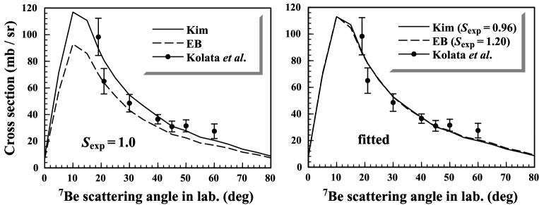
Figure 2: Angular distribution of the ⁷Be fragment in the laboratory frame. The solid and dashed lines represent the results of CDCC calculation with the parameter set of Kim and Esbensen-Bertsch (EB), respectively, for ⁸B single particle potential. Results in the left panel correspond to $S_{\rm exp}=1$ and those with appropriate values of $S_{\rm exp}$, i.e., 0.96 for Kim and 1.20 for EB, are shown in the right panel. The experimental data are taken from Ref. [12].

In Fig. 2 we show the results of the angular distribution of ⁷Be fragment, integrated over scattering angles of $p$ and excitation energies of the ⁷Be + $p$ system. In the left panel the results with the ⁸B wave functions by Kim et al. [19] (solid line) and Esbensen and Bertsch [16] (dashed line), with the spectroscopic factor $S_{\rm exp}$ equal to unity, are shown. After $\chi^{2}$ fitting, one obtains the results in the right panel; one sees that both calculations very well reproduce the experimental data. The resultant $S_{\rm exp}$ is 0.96 and 1.20 with the ⁸B wave functions by Kim and Esbensen-Bertsch, respectively, showing quite strong dependence on ⁸B models. In contrast to that, the ANC $C$ calculated by $C=S_{\rm exp}^{1/2}b$ with $b$ the single-particle ANC, is found to be almost independent of the choice of ⁸B wave functions, i.e., $C=0.59\pm 0.004$ (fm^-1/2). Thus, one can conclude that the ANC method works in the present case within 1% of error.

Following Ref. [3] we obtained the following result:

$$S_{17}(0)=22.83\pm 0.17({\rm ANC})\pm 0.34({\rm CDCC})\pm 2.28({\rm expt})\;\;({\rm eVb}),$$

where the uncertainties from the choice of the modelspace of CDCC calculation (1.5%) and the systematic error of the experimental data (10%) are also included. Although the quite large experimental error prevents one from determining $S_{17}(0)$ with the required accuracy (5%), the CDCC + ANC method turned out to be a powerful technique to determine $S_{17}(0)$ with small theoretical uncertainties. More careful analysis in terms of the charge distribution of ⁷Be, nuclear optical potentials and roles of the intrinsic spins of the constituents, are being made and more reliable $S_{17}(0)$ will be reported in a forthcoming paper.

3 Hybrid calculation for Coulomb dissociation

In Sec. 2 we showed that the CDCC + ANC analysis for the ⁸B dissociation at 25.8 MeV gives $S_{17}(0)$ with good accuracy, being free from rather ambiguous assumptions made in the previous analyses using VPT. In Ref. [6] it was shown that the ANC method works well for one-nucleon breakup reactions at intermediate energies. Also CDCC turned out to almost perfectly reproduce the parallel-momentum distribution of ⁷Be fragment from ²⁰⁸Pb(⁸B,⁷Be$+p$)²⁰⁸Pb at 44 MeV/nucleon [11]. Thus, it is expected that accurate determination of $S_{17}(0)$ can be done by the CDCC + ANC analysis of ⁸B Coulomb dissociation measured at RIKEN [9], GSI [10] and MSU [11].

From a practical point of view, however, CDCC calculation including long-ranged Coulomb coupling-potentials requires extremely large modelspace rather difficult to handle; typically the number of partial waves is 15,000 for the MSU data [11]. Although interpolation technique for angular momentum reduces the number of CC equations to be solved in terms of $J$, those with huge angular momenta are rather unstable and careful treatment is necessary. In this sense, it seems almost impossible to apply CDCC to the GSI data at 250 MeV/nucleon, where $J_{\rm max}$ is expected to exceed 100,000.

On the contrary, semi-classical approaches, expected to work quite well at intermediate energies, are free from any problems concerned with huge angular momenta. The accuracy of such semi-classical calculations, however, is difficult to be evaluated quantitatively, although one may naively estimate the error is only less than about 10% or so. It should be noted that our goal is to determine $S_{17}(0)$ with more than 95% accuracy, which requires definite estimation of the error of the calculation.

In this section we propose HY calculation of ⁸B dissociation at intermediate energies, constructing HY scattering amplitude ($T$ matrix) from partial amplitudes with quantum-mechanical (QM) and eikonal (EK) CC calculations; for the latter we use a new version of CDCC, that is, the Eikonal-CDCC method (E-CDCC). The formalism of E-CDCC and calculation of the HY amplitude are described in subsection 3.1 and the validity of the hybrid calculation is tested for ⁵⁸Ni(⁸B,⁷Be$+p$)⁵⁸Ni at 240 MeV in subsection 3.2.

3.1 The Eikonal-CDCC method and construction of hybrid scattering amplitude

We start with the expansion of the total wave function $\Psi$:

$$\Psi({\bf R},{\bf r})=\sum_{i\ell m}\Phi_{i,\ell m}({\bf r})e^{-i(m-m_{0})\phi_{R}}\chi_{i\ell m}(R,\theta_{R}),$$ (7)

where $m$ is the projection of $\ell$ on the $z$-axis taken to be parallel to the incident beam; $\Phi_{i,\ell m}$ is the discretized internal-wave-function of c, calculated just in the same way as in the standard CDCC. The symbol “ $\hat{}$ ” used in subsection 2.2, which denotes a discretized quantity, is omitted here for simplicity.

We make the following EK approximation:

$$\chi_{c}(R,\theta_{R})\approx\psi_{c}(b,z){\displaystyle\frac{1}{(2\pi)^{3/2}}}e^{i{\bf K}_{c}(b)\cdot{\bf R}},$$ (8)

where $c$ denotes channels {$i$, $\ell$, $m$} together and the wave number $K_{c}$ is defined by

$${\displaystyle\frac{\hbar^{2}}{2\mu}}K_{c}^{2}(b)=E-\epsilon_{i,\ell}-{\displaystyle\frac{\hbar^{2}}{2\mu}}{\displaystyle\frac{(m-m_{0})^{2}}{b^{2}}}$$ (9)

with $b$ the impact parameter; the direction of ${\bf K}_{c}$ is assumed to be parallel to the $z$-axis.

Inserting Eqs. (7) and (8) into a three-body Schrödinger equation and neglecting the second order derivative of $\psi_{c}$, one can obtain the following E-CDCC equations:

$${\displaystyle\frac{i\hbar^{2}}{\mu}}K_{c}^{(b)}{\displaystyle\frac{d}{dz}}\psi_{c}^{(b)}(z)=\sum_{c^{\prime}}{\cal F}^{(b)}_{cc^{\prime}}(z)\;\psi_{c^{\prime}}^{(b)}(z)e^{i\left(K_{c^{\prime}}^{(b)}-K_{c}^{(b)}\right)z}$$ (10)

for all $c$ including $c_{0}$, with ${\cal F}^{(b)}_{cc^{\prime}}(z)=\langle\Phi_{c}({\bf r})|U|\Phi_{c^{\prime}}({\bf r})\rangle_{\bf r}\exp[i(m^{\prime}-m)\phi_{R}]$. We put $b$ in a superscript since it is not a dynamical variable but an input parameter. Equations (10) are solved with the boundary condition $\psi_{c}^{(b)}(-\infty)=\delta_{c0}$. Since the E-CDCC equations are first-order differential ones and contain no coefficients with huge angular momenta, they can easily and safely be solved.

Using the solutions of Eq. (10), the scattering amplitude with E-CDCC is given by

$$f_{c0}^{\rm E}=-{\displaystyle\frac{\mu}{2\pi\hbar^{2}}}\int\sum_{c^{\prime}}{\cal F}^{(b)}_{cc^{\prime}}(z)\,e^{-i(m-m_{0})\phi_{R}}e^{i({\bf K_{c^{\prime}}^{(b)}}-{\bf K_{c}^{\prime(b)}})\cdot{\bf R}}\,\psi_{c^{\prime}}^{(b)}(z)d{\bf R}.$$ (11)

Making use of the following forward-scattering approximation:

$$({\bf K_{c^{\prime}}^{(b)}}-{\bf K_{c}^{\prime(b)}})\cdot{\bf R}\approx-K_{c}^{(b)}\theta_{f}b\cos{\phi_{R}}+(K_{c^{\prime}}^{(b)}-K_{c}^{(b)})z,$$ (12)

one obtains

$$f_{i\ell m,i_{0}\ell_{0}m_{0}}^{\rm E}={\displaystyle\frac{1}{2\pi i}}\int\!\!\int K_{i\ell m}^{(b)}e^{-i(m-m_{0})\phi_{R}}e^{-iK_{i\ell m}^{(b)}\theta_{f}b\cos{\phi_{R}}}\left({\cal S}_{i\ell m,i_{0}\ell_{0}m_{0}}^{(b)}\!\!-\delta_{ii_{0}}\delta_{\ell\ell_{0}}\delta_{mm_{0}}\right)bdbd\phi_{R},\\$$ (13)

where the EK $S$-matrix elements are defined by ${\cal S}_{i\ell m,i_{0}\ell_{0}m_{0}}^{(b)}\equiv\psi_{i\ell m}^{(b)}(\infty)$.

We then discretize $f^{\rm E}$:

$$f_{i\ell m,i_{0}\ell_{0}m_{0}}^{\rm E} = {\displaystyle\frac{1}{2\pi i}}\sum_{L}K_{i\ell m}^{(b_{L}^{\rm mid})}\left[\int e^{-i(m-m_{0})\phi_{R}}e^{-iK_{i\ell m}^{(b_{L}^{\rm mid})}\theta_{f}b_{L}\cos{\phi_{R}}}d\phi_{R}\right]$$ (14)

$$\times{}\left({\cal S}_{i\ell m,i_{0}\ell_{0}m_{0}}^{(b_{L}^{\rm mid})}-\delta_{ii_{0}}\delta_{\ell\ell_{0}}\delta_{mm_{0}}\right)\int_{b_{L}^{\rm min}}^{b_{L}^{\rm max}}bdb,$$

where $b_{L}^{\rm min}$, $b_{L}^{\rm max}$ and $b_{L}^{\rm mid}$ are defined through $K_{i\ell m}^{(b_{L}^{\rm min})}b_{L}^{\rm min}=L$, $K_{i\ell m}^{(b_{L}^{\rm max})}b_{L}^{\rm max}=L+1$ and $K_{i\ell m}^{(b_{L}^{\rm mid})}b_{L}^{\rm mid}=L+1/2$, respectively. In deriving Eq. (14) we neglected the $b$-dependence of $K_{i\ell m}^{(b)}$, $\exp[-iK_{i\ell m}^{(b)}\theta_{f}b\cos{\phi_{R}}]$ and ${\cal S}_{i\ell m,i_{0}\ell_{0}m_{0}}^{(b)}$ within a small size of $b$ corresponding to each $L$. After manipulation one can obtain

$$f_{i\ell m,i_{0}\ell_{0}m_{0}}^{\rm E}\!\!\approx{\displaystyle\frac{2\pi}{iK_{0}}}\sum_{L}{\displaystyle\frac{K_{0}}{K_{i\ell m}^{(b_{L}^{\rm mid})}}}\sqrt{{\displaystyle\frac{2L+1}{4\pi}}}i^{(m-m_{0})}Y_{L\,m\!-m_{0}}(\hat{\bf K}^{\prime})\left({\cal S}_{i\ell m,i_{0}\ell_{0}m_{0}}^{(b_{L}^{\rm mid})}\!\!-\delta_{ii_{0}}\delta_{\ell\ell_{0}}\delta_{mm_{0}}\right),\\$$

which has a similar form to that of the standard CDCC:

$$f^{\rm Q}_{i\ell m,i_{0}\ell_{0}m_{0}}\!\!\!\!\! = \!\!\!{\displaystyle\frac{2\pi}{iK_{0}}}\sum_{L}\sum_{J=|L-\ell|}^{L-\ell}\sum_{L_{0}=|J-\ell_{0}|}^{J-\ell_{0}}\sqrt{{\displaystyle\frac{2L_{0}+1}{4\pi}}}(L_{0}0\ell_{0}m_{0}|Jm_{0})(L\;m_{0}\!\!-\!m\;\ell m|Jm_{0})$$ (15)

$$\!\!\!\hskip 45.5244pt{}\times(S_{iL\ell,i_{0}L_{0}\ell_{0}}^{J}-\delta_{ii_{0}}\delta_{LL_{0}}\delta_{\ell\ell_{0}})(-)^{m-m_{0}}Y_{L\,m\!-m_{0}}(\hat{\bf K}^{\prime}).$$

The construction of the HY scattering amplitude $f^{\rm H}$ can be done by:

$$f_{i\ell m,i_{0}\ell_{0}m_{0}}^{\rm H}\equiv\sum_{L\leq L_{\rm C}}f_{L}^{\rm Q}+\sum_{L>L_{\rm C}}f_{L}^{\rm E},$$ (16)

where $f_{L}^{\rm Q}$ ($f_{L}^{\rm E}$) is the $L$-component of $f^{\rm Q}$ ($f^{\rm E}$) and $L_{\rm C}$ represents the connecting point between the QM and EK calculations, which is chosen so that $f_{L}^{\rm E}$ coincides with $f_{L}^{\rm Q}$ for $L>L_{\rm C}$. One sees that Eq. (16) includes all QM effects necessary through $f_{L}^{\rm Q}$, and also interference between the lower and higher $L$-regions. It should be noted that derivation of Eq. (3.1), which leads one to Eq. (16) rather straightforwardly, is one of the most important features of E-CDCC. Actually, the present EK calculation is very simple, i.e., E-CDCC equations (10) contain no correction terms to the straight-line approximation. However, this is not a defect but a merit of E-CDCC, since such a simplest calculation is enough to describe scattering processes, if combined with the result of the QM calculation taking an appropriate $L_{\rm C}$.

In the above formulation we neglected the Coulomb distortion. In order to include it, we use $\chi_{c}(R,\theta_{R})\approx\psi_{c}(b,z)(2\pi)^{-3/2}\phi_{c}^{\rm C}(b,z)$ instead of Eq. (8) [20], where $\phi_{c}^{\rm C}$ is the Coulomb wave function. The formulation of $f^{\rm E}$ can then be done just in the same way as above.

3.2 Numerical test for the hybrid calculation

In order to see the validity of the HY calculation with CDCC and E-CDCC, we analyze ⁵⁸Ni(⁸B,⁷Be$+p$)⁵⁸Ni at 240 MeV. The number of bin-states of ⁸B is 16, 8 and 8 for s-, p- and d-states, respectively, and $L_{\rm max}$ is 4000. As for the ⁸B wave function, the parameter set by Kim et al. [19] was adopted. For nuclear interaction between ⁷Be and ⁵⁸Ni we used the global potential for ⁷Li scattering by Cook et al. [21]. Other parameters are taken just the same as in subsection 2.3.

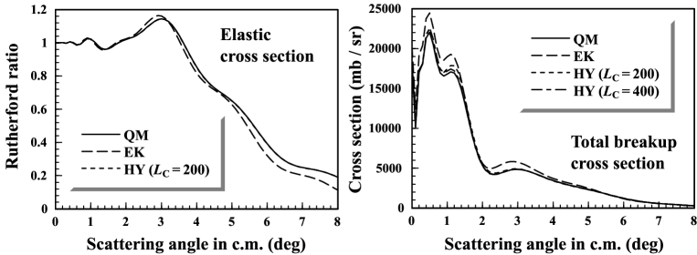
Figure 3: Angular distribution of the elastic (left panel) and total breakup (right panel) cross sections for ⁵⁸Ni(⁸B,⁷Be$+p$)⁵⁸Ni at 240 MeV. The solid and dashed lines show, respectively, the results of the QM and EK calculations. The dotted (dash-dotted) line represents the HY result with $L_{\rm C}=200$ (400).

In the left and right panels in Fig. 3 we show the elastic cross section (Rutherford ratio) and the total breakup one, respectively, as a function of scattering angle in the center-of mass (c.m.) frame. The solid, dashed and dotted lines represent the results of the QM, EK and HY calculations, where $L_{\rm C}$ is taken to be 4000, 0 and 200, respectively. In the right panel the result of the HY calculation with $L_{\rm C}=400$ is also shown by the dash-dotted line. The agreement between the QM and HY calculations with an appropriate value of $L_{\rm C}$ for the latter, namely, 200 (400) for elastic (breakup) cross section, is excellent; the error is only less than 1%. One also sees that difference between the EK and QM results is appreciable. Since the present EK calculation is quite simple, as mentioned in the previous subsection, this does not directly show the fail of EK approximation. However, it seems quite difficult for EK calculation to obtain “perfect” agreement with the result of the QM one. On the contrary, the HY calculation turned out to be applicable to analyses of ⁸B dissociation to extract $S_{17}(0)$, where very high accuracy is required.

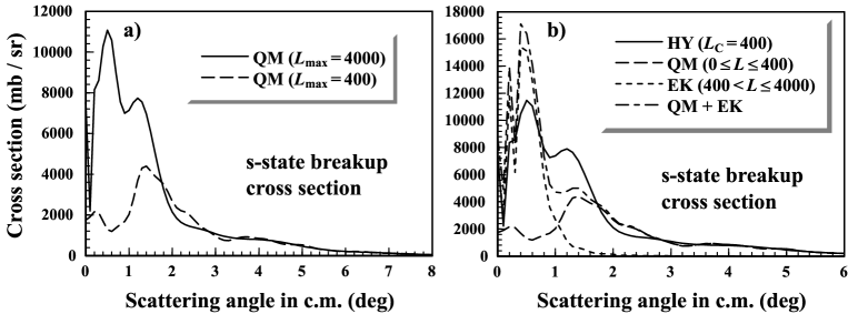
Figure 4: a) QM results for the s-state breakup cross section with $L_{\rm max}=4000$ (solid line) and 400 (dashed line). b) The s-state breakup cross sections by the QM calculation with $0\leq L\leq 400$ (dashed line) and the EK calculation with $400<L\leq 4000$ (dotted line). The dash-dotted line is the incoherent sum of the dashed and dotted lines and the solid line is the HY result with $L_{\rm C}=400$, namely, the coherent sum of the two.

We show in the left panel of Fig. 4 the s-state breakup cross sections by the QM calculation; the solid and dashed lines correspond to the calculation with $L_{\rm max}=4000$ and 400, respectively. One sees big difference between the two, which shows that the partial scattering amplitudes for larger $L$ indeed has an essential contribution to the breakup cross section. In the right panel we show the s-state breakup cross sections by the QM calculation with $0\leq L\leq 400$ (dashed line) and the EK calculation with $400<L\leq 4000$ (dotted lines). The dash-dotted line is the incoherent sum of the two, which deviates from the HY result shown by the solid line. Thus, one sees that the essence of the present HY calculation is the construction of the HY scattering amplitude not the HY cross section.

We show in Fig. 5 the p-state breakup cross sections by the QM calculation with (dashed line) and without (solid line) adiabatic (AD) approximation. One sees that the AD approximation increases the breakup cross section about 10% at forward angles. The oscillation shown by the dashed line seems to indicate the AD calculation is not valid in the present case, probably for higher partial waves. We found just the same features in the EK calculation.

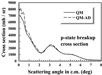
Figure 5: The p-state breakup cross sections by the QM calculation with (dashed line) and without (solid line) AD approximation.

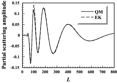
Figure 6: Comparison between $f_{L}^{\rm Q}$ (solid line) and $f_{L}^{\rm E}$ (dashed line) for the {$\ell$, $m$} $=$ {$\ell_{0}$, $m_{0}$} $=$ {1, 0} component.

Comparison between $f_{L}^{\rm Q}$ (solid line) and $f_{L}^{\rm E}$ (dashed line) in Eq. (16), corresponding to the {$\ell$, $m$} $=$ {$\ell_{0}$, $m_{0}$} $=$ {1, 0} component, is made in Fig. 6. One sees that the difference between $f_{L}^{\rm Q}$ and $f_{L}^{\rm E}$ is appreciable for smaller $L$, around 100 in particular, and as the larger $L$ becomes, the better agreement is obtained. For $L\geq 400$, the difference is not visible, which is consistent with the result shown in the right panel of Fig. 3.

Thus, the HY calculation of ⁸B Coulomb dissociation turned out to allow one to make efficient and accurate analysis. The method is expected to be applicable to the experimental data measured at not only RIKEN and MSU (at several tens of MeV/nucleon) but also GSI (at 250 MeV/nucleon), i.e., systematic analysis of ⁸B Coulomb dissociation for wide energy regions can be done.

4 Summary and Conclusions

In the present paper we propose systematic analysis of ⁸B Coulomb dissociation with the Asymptotic Normalization Coefficient (ANC) method. An important advantage of the use of the ANC method is that one can extract the astrophysical factor $S_{17}(0)$ evaluating its uncertainties quantitatively, in contrast to the previous analyses with the Virtual Photon Theory (VPT).

In order to make accurate analysis of the measured spectra in dissociation experiments, we use the method of Continuum-Discretized Coupled-Channels (CDCC), which was developed by Kyushu group. The CDCC + ANC analysis was found to work very well for ⁵⁸Ni(⁸B,⁷Be$+p$)⁵⁸Ni at 25.8 MeV measured at Notre Dame, and we obtained $S_{17}(0)=22.83\pm 0.51({\rm theo})\pm 2.28({\rm expt})$ (eVb), which is consistent with both the latest recommended value $19^{+4}_{-2}$ eVb [22] and recent results of direct measurements [23, 24].

The CDCC + ANC analysis is expected to work well also at intermediate energies. From a practical point of view, however, CDCC calculation for ⁸B Coulomb dissociation at several tens of MeV/nucleon requires extremely large modelspace, typically about 15,000 partial waves are needed. In order to make efficient analysis at intermediate energies, we introduce a new version of CDCC, that is, the Eikonal-CDCC method (E-CDCC). E-CDCC describes the center-of-mass (c.m.) motion between the projectile and the target nucleus by a straight-line and treats the excitation of the projectile explicitly, by constructing discretized-continuum-states same as in CDCC. The resultant E-CDCC equations are easily and safely be solved, since they have a first-order differential form and no huge angular momenta, in contrast to the CDCC equations. Inclusion of the Coulomb distortion can be done with the use of Coulomb wave functions instead of plane waves in eikonal (EK) approximation.

One of the most important features of E-CDCC is that the resultant scattering amplitude $f^{\rm E}$ has a very similar form to the quantum-mechanical (QM) one, i.e., $f^{\rm E}$ is expressed by the sum of partial amplitudes $f_{L}^{\rm E}$, using relation between the angular momentum $L$ and the impact parameter $b$. This allows one to construct the hybrid (HY) amplitude $f^{\rm H}$ rather straightforwardly; $f^{\rm H}$ is given by the sum of the partial amplitudes calculated by CDCC for smaller $L$, $\sum_{L\leq L_{\rm C}}f_{L}^{\rm Q}$, and those by E-CDCC for larger $L$, $\sum_{L>L_{\rm C}}f_{L}^{\rm E}$, where $L_{\rm C}$ is the connecting value. The HY calculation make the CDCC + ANC analysis much simple, retaining its accuracy; all QM effects necessary can be included through $f_{L}^{\rm Q}$.

The validity of the HY calculation is tested for ⁵⁸Ni(⁸B,⁷Be$+p$)⁵⁸Ni at 240 MeV. The HY calculation turned out to “perfectly” reproduce the elastic and total breakup cross sections obtained by the QM one, namely, the error is only less than 1%; the appropriate value of $L_{\rm C}$ is found to be 400 (200) for the total-breakup (elastic) cross section, which is much smaller than the required maximum value of $L$, i.e., $L_{\rm max}=4000$. Calculation with a HY cross section, not HY amplitude, was found to fail to reproduce the corresponding QM result, which shows the importance of the interference between the lower (QM) and higher (EK) regions of $L$.

In conclusion, systematic analysis of ⁸B Coulomb dissociation with the ANC method and the HY Coupled-Channels (CC) calculation is expected to accurately determine $S_{17}(0)$, with reliable evaluation of its uncertainties. An extracted $S_{17}(0)$ from the RIKEN, MSU and GSI data, combined with that from the Notre Dame experiment, will be reported in near future.

References

- [1] J. N. Bahcall et al., Astrophys. J. 555, 990 (2001) and references therein.
- [2] J. N. Bahcall et al., JHEP 0108, 014 (2001) [arXiv:hep-ph/0106258]; JHEP 0302, 009 (2003) [arXiv:hep-ph/0212147].
- [3] H. M. Xu et al., Phys. Rev. Lett. 73, 2027 (1994).
- [4] A. Azhari et al., Phys. Rev. Lett. 82, 3960 (1999).
- [5] A. Azhari et al., Phys. Rev. C 60, 055803 (1999);
- [6] L. Trache et al., Phys. Rev. Lett. 87, 271102 (2001).
- [7] K. Ogata et al., Phys. Rev. C 67, R011602 (2003).
- [8] M. Kamimura et al., Prog. Theor. Phys. Suppl. 89 1 (1986); N. Austern et al., Phys. Rep. 154, 125 (1987).
- [9] T. Motobayashi et al., Phys. Rev. Lett. 73, 2680 (1994); T. Kikuchi et al., Eur. Phys. J. A 3, 209 (1998).
- [10] N. Iwasa et al., Phys. Rev. Lett. 83, 2910 (1999).
- [11] B. Davids et al., Phys. Rev. Lett. 86, 2750 (2001); Phys. Rev. C 63, 065806 (2001).
- [12] J. von Schwarzenberg et al., Phys. Rev. C 53, 2598 (1996); J. J. Kolata et al., Phys. Rev. C 63, 024616 (2001).
- [13] Y. Iseri et al., Prog. Theor. Phys. Suppl. 89, 84 (1986).
- [14] R. A. D. Piyadasa et al., Phys. Rev. C 60, 044611 (1999).
- [15] N. Austern et al., Phys. Rev. Lett. 63, 2649(1989); Phys. Rev. C 53, 314 (1996).
- [16] H. Esbensen and G. F. Bertsch, Phys. Rev. C 59, 3240 (1999).
- [17] F. D. Becchetti and G. W. Greenlees, Phys. Rev. 182, 1190 (1969).
- [18] Z. Moroz et al., Nucl. Phys. A381, 294 (1982).
- [19] K. H. Kim et al., Phys. Rev. C 35, 363 (1987).
- [20] M. Kawai, private communication (2003).
- [21] J. Cook, Nucl. Phys. A388, 153 (1982).
- [22] E. G. Adelberger et al., Rev. Mod. Phys. 70, 1265 (1998).
- [23] A. R. Junghans et al., Phys. Rev. Lett. 88, 041101 (2002).
- [24] L. T. Baby et al., Phys. Rev. C 67, 065805 (2003).