Non-equilibrated post freeze out distributions

Abstract

We discuss freeze out on the hypersurface with time-like normal vector, trying to answer how realistic is to assume thermal post freeze out distributions for measured hadrons. Using simple kinetic models for gradual freeze out we are able to generate thermal post FO distribution, but only in highly simplified situation. In a more advanced model, taking into account rescattering and re-thermalization, the post FO distribution gets more complicated. The resulting particle distributions are in qualitative agreement with the experimentally measured pion spectra. Our study also shows that the obtained post FO distribution functions, although analytically very different from the Jüttner distribution, do look pretty much like thermal distributions in some range of parameters.

1 Introduction

Since the very beginning of heavy ion collision physics fluid dynamical models were widely used for simulation of such reactions. Their advantage is that one can vary flexibly the Equation of State (EoS) of the matter and test its consequences on the reaction dynamics and the outcome. This makes fluid dynamical models a very powerful tool to study possible phase transitions in heavy ion collisions - such as the liquid-gas or the Quark-Gluon Plasma (QGP) phase transition. For highest energies, achieved nowadays at RHIC, hydrodynamic calculations give a good description of the observed radial and elliptic flows Sollfrank-BigHydro ; Schlei-BigHydro ; Kolb-UU ; Kolb-LowDensity ; Kolb-Radial ; Htoh , in contrast to microscopic models, like HIJING Molnar-Elliptic and UrQMD UrQMD-Elliptic .

Freeze out (FO) process is an important and necessary part of the fluid dynamical modeling. Generally saying, fluid dynamical models are determined by the initial state, EoS and the way FO is realized, in addition to well known fluid dynamical equations. FO describes the last stages of the reaction, when the matter becomes so dilute and cold that particles do not interact anymore, their momentum distribution freezes out, and particles stream freely toward the detectors. FO models allow the evaluation of two-particle correlation data, different flow analyzes, transverse momentum and transverse mass spectra and other observables. There are many different theoretical approaches for the freeze out problem. Sometimes these approaches are oversimplified to the extent that conservation of energy and momentum is violated (see Ref. FO2 ; FO3 for an overview).

A basic standard assumption in fluid dynamical modeling of heavy ion collisions is that freeze out happens across a hypersurface in space-time. Such a hypersurface is an idealization of a layer of finite thickness (of the order of at least mean free path or collision time) where the frozen-out particles are formed and the interactions in the matter become negligible. The dynamics of this layer is described in different kinetic models such as Monte Carlo models BB95 ; BB97 or four-volume emission models BC82 ; GH95 ; GH96 ; GH97 ; He97 . Under such an assumption FO can be pictured as a discontinuity in relativistic flow, where the kinetic properties of the matter, such as energy density or flow velocity change suddenly.

It took a long time to develop general theory of discontinuities in the relativistic flow. The story goes like this. In 1948 Taub Ta48 discussed discontinuities across propagating hypersurfaces with space-like normal vectors. If one applies Taub’s formalism to FO hypersurface with time-like normal vector, one gets a usual Taub adiabat, but the equation of the Rayleigh line yields imaginary values for the particle current across the front. Thus, these hypersurfaces were thought unphysical. However more recently, Taub’s approach has been generalized to these hypersurfaces as well Cs87 and the imaginary particle currents arising from the equation of the Rayleigh line were eliminated. Thus, it is possible to take into account conservation laws exactly across any surface of discontinuity in relativistic flow. The corresponding equations are

$$T_{pre}^{\mu\nu}d\sigma_{\nu}=T_{post}^{\mu\nu}d\sigma_{\nu}\,\,,~{}~{}$$ (1)

$$n_{pre}u_{pre}^{\mu}d\sigma_{\mu}=n_{post}u_{post}^{\mu}d\sigma_{\mu}\,\,,$$ (2)

where $d\sigma^{\mu}$ is the unit 4-vector normal to the discontinuity hypersurface,

$$T^{\mu\nu}=(\epsilon+p)u^{\mu}u^{\nu}-pg^{\mu\nu}$$ (3)

is the energy-momentum tensor,

$$N^{\mu}=nu^{\mu}$$ (4)

is a baryon current (usually in heavy ion collision modeling we neglect electric charge current) These consist of local thermodynamical fluid quantities: the energy density $\epsilon$, pressure $p$, baryonic density $n$ and the collective four-velocity $u^{\mu}=\frac{1}{\sqrt{1-\vec{v}^{2}}}(1,\vec{v})$.

Since 1974 people were using the Cooper-Frye formula CF74 to calculate final particle spectra. Much later it was realized that the Cooper-Frye FO description has a conceptual problem of negative contributions, when it is applied to the FO hypersurface with space-like normal vector Bu96 ; FO2 ; FO1 ; FO3 ; FO4 ; FO5 ; ref18 ; bug . This leads to the non-equilibrated cut-off post FO distributions:

$$f_{FO}(\vec{r},p;T,n,u^{\nu},d\sigma^{\mu})=f_{FO}(\vec{r},p;T,n,u^{\nu})\Theta(p^{\mu}\ d\sigma_{\mu})\ .$$ (5)

The simplest example of such cut-off distribution is the cut Jüttner distribution Jutt , proposed in Ref. Bu96 . In Refs. FO1 ; FO3 ; FO4 ; FO5 it was shown that one can obtain cut Jüttner post FO distribution in a oversimplified kinetic model. If one improves this model, taking into account rescattering and re-thermalization, or if one uses more realistic four-volume emission model FO3 , then final distributions have more complicated form, although they are cut-off as required. Unfortunately, so far we do not have good analytical expression to fit post FO distributions for the hypersurface with space-like (or, generally, any type of) normal vector. Therefore in most calculations scientists prefer to model FO based on time-like hypersurfaces. For the ultra-relativistic heavy ion collisions this is justified by the Bjorken model, where the natural choice of FO hypersurface is $\tau=\tau_{FO}$.

In this paper we ask the following question. Well, we know now that FO through the hypersurface with space-like normal vector leads to non-equilibrated post FO distributions, but can we really assume thermal post FO distributions if the FO hypersurface is time-like? This is not restricted by general theory, but how realistic such an assumption is? From the experimental data we know that pion and charged hadron (which are actually pion dominated) transverse mass spectra both at SPS and at RHIC spectra ; summspectra are not the Jüttner type - the slope parameter is decreasing with increasing $p_{t}$.

We generalize the simple model presented in Refs. FO1 ; FO3 ; FO4 ; FO5 for the FO hypersurface with time-like normal vector (the model is also not 1D anymore). The philosophy of this work is also similar - first we will show that in the oversimplified model the obtained post FO spectra are really thermal ones. Then in more realistic model, taking into account rescattering in the still interacting gas, we will obtain post FO distribution in the more complicated non-equilibrated form, which is in qualitative agreement with experimental data, mentioned above. Actually the main goal of this work is not quantitative calculations, but a qualitative understanding of the phenomenon in simple models.

2 Simple freeze out model

As it was mentioned above our basic model is in some sense similar to the one discussed in Refs. FO1 ; FO3 ; FO4 ; FO5 , but on the other hand it is much more realistic and also habitual for the people working in ultra-relativistic heavy ion collision field. Instead of very special geometry (1D, infinitely long tube with particle source on the left end and vacuum on the right one) used in Refs. FO1 ; FO3 ; FO4 ; FO5 , this model can be combined with any relativistic hydrodynamical model. Below we will use proper time coordinate keeping in mind the Bjorken hydrodynamical model, as the simplest but still reliable one, although the similar treatment could be done for any pre FO state.

Let assume that at some moment $\tau=\tau_{0}$ our matter is still completely equilibrated and described by the thermal distribution $f_{Juttner}(\tau_{0},\vec{r},p,T,n,u^{\mu})$. Starting from this moment matter starts to gradually freeze out. At each particular moment $\tau_{i}$ the FO hypersurface will be $\tau=\tau_{i}$, and we will follow this hypersurface, i.e. we will describe our system from the reference frame of the front (RFF), where normal vector is $d\sigma_{\mu}=(1,0,0,0)$. We can describe the FO kinetics of such a system assuming that we have two components of our distribution GH95 ; GH96 ; GH97 ; FO1 ; FO3 ; FO4 ; FO5 : $f_{free}(\tau,\vec{r},p)$, describing frozen out particles, and $f_{int}(\tau,\vec{r},p)$, describing particles, which still interact (below we will use shorter notations, $f_{free}(\tau)$ and $f_{int}(\tau)$, but the meaning is the same). At the initial moment, $\tau=\tau_{0}$, the distribution $f_{free}$ vanishes exactly and $f_{int}(\tau_{0})=f_{Juttner}(\tau_{0},\vec{r},p,T,n,u^{\mu})$. In this work we will use an extended definition of the classical Jüttner distribution Jutt , which is adequate at ultra-relativistic energies and allow for particle creation. Thus the particle density, which depends on $T$, is not the same as the conserved baryon charge density, $n$. Then, $f_{int}$ gradually disappears and $f_{free}$ gradually builds up as $\tau$ increases. The most simple kinetic model describing the evolution of such a system is the following:

$$\partial_{\tau}f_{int}(\tau)=-\frac{1}{\tau_{f}}f_{int}(\tau)\,,$$

(6)

$$\partial_{\tau}f_{free}(\tau)=\frac{1}{\tau_{f}}f_{int}(\tau)\,,$$

where $\tau_{f}$ is a parameter with dimension of time determining how fast particles freeze out. It is of the order of collision time. In general case $\tau_{f}$ may depend on particle density and momentum of the particle, but in our simple model we neglect such effects and consider $\tau_{f}=const$. Our assumption becomes particularly bad for the large times, when the particle density is very low - we will discuss this problem separately in section 2.3. If this approximation is not done, i.e. the relaxation time is assumed to be momentum and density dependent, that would be a large step towards the full solution of the BTE, which is then a much more involved problem, and in most cases cannot be performed analytically. Nevertheless even this strongly simplifying assumption leads to nontrivial results as we shall see later.

The interacting component, $f_{int}$, will gradually freeze out in an exponential rarefaction with time.

$$f_{int}(\tau)=f_{Juttner}(\tau_{0})e^{-\frac{\tau-\tau_{0}}{\tau_{f}}}.$$ (7)

Then

$$f_{free}(\tau)=f_{Juttner}(\tau_{0})\left(1-e^{-\frac{\tau-\tau_{0}}{\tau_{f}}}\right)\,.$$ (8)

At $\tau\longrightarrow\infty$ the distribution $f_{free}$ will tend to the original Jüttner distribution, while $f_{int}$ will vanish. The frozen out particles keep their velocities and consequently the volume occupied by the frozen out matter will gradually increase with time.

This is a highly unrealistic model, similar to the one resulting in the cut Jüttner distribution in Refs. FO1 ; FO3 ; FO4 ; FO5 for the FO hypersurface with space-like normal vector. We can improve this model taking into account rescattering in the interacting component in the same way as it was done in the References above.

2.1 Freeze out model with rescattering

The assumption that the interacting part of the distribution, $f_{int}$, remains after some drain the same Jüttner distribution with decreased amplitude is, of course, highly unrealistic. As suggested in Refs. FO1 ; FO3 ; FO4 ; FO5 rescattering within this component will lead to re-thermalization and re-equilibration of this component. Thus, the evolution of the component $f_{int}$ is determined both by the drain term and the re-equilibration. If we include the collision terms explicitly into the transport equations (6) this in general case leads to a combined set of integro-differential equations. We can, however, take advantage of the relaxation time approximation to simplify the description of the dynamics. In this framework the two components of the momentum distribution develop according to the modified coupled differential equations:

$$\partial_{\tau}f_{int}(\tau)=-\frac{1}{\tau_{f}}f_{int}(\tau)+\left[f_{eq}(\tau)-f_{int}(\tau)\right]\frac{1}{\tau_{r}}\,,$$

(9)

$$\partial_{\tau}f_{free}(\tau)=\frac{1}{\tau_{f}}f_{int}(\tau)\,.$$

Thus, the interacting component of the momentum distribution, described by eq. (9), shows the tendency to approach an equilibrated distribution with a relaxation time $\tau_{r}$. Of course due to the energy, momentum and conserved particle drain, this distribution, $f_{eq}(\tau)$ is not the same as the initial Jüttner distribution, but its parameters, $n_{eq}(\tau)$, $T_{eq}(\tau)$ and $u^{\mu}_{eq}(\tau)$, change as required by the conservation laws.

If we do not have collision or relaxation terms in our transport equation then the conservation laws are trivially satisfied, because the change of the full distribution function is $\partial_{\tau}f=\partial_{\tau}f_{int}(\tau)+\partial_{\tau}f_{free}(\tau)=0$. If, however, collision or relaxation terms are present, these contribute to the change of $T^{\mu\nu}$ and $N^{\mu}$, and this should be considered in the modified distribution function $f_{int}(\tau)$. In this case from the conservation laws we get:

$$dN_{int}^{\mu}=-dN_{free}^{\mu}=-\frac{d\tau}{\tau_{f}}\int\frac{d^{3}p}{p_{0}}p^{\mu}f_{int}(\tau)=-\frac{d\tau}{\tau_{f}}N_{int}^{\mu}$$ (10)

and

$$dT_{int}^{\mu\nu}=-dT_{free}^{\mu\nu}=-\frac{d\tau}{\tau_{f}}\int\frac{d^{3}p}{p_{0}}p^{\mu}p^{\nu}f_{int}(\tau)=-\frac{d\tau}{\tau_{f}}T_{int}^{\mu\nu}\,,$$ (11)

where we used kinetic definitions of $N^{\mu}$ and $T^{\mu\nu}$. The above equations can be easily solved:

$$N_{int}^{\mu}(\tau)=N^{\mu}(\tau_{0})e^{-\frac{\tau-\tau_{0}}{\tau_{f}}}$$ (12)

and

$$T_{int}^{\mu\nu}(\tau)=T^{\mu\nu}(\tau_{0})e^{-\frac{\tau-\tau_{0}}{\tau_{f}}}\,.$$ (13)

2.2 Immediate re-thermalization limit

As a first approximation to this solution let us assume that $\tau_{r}\ll\tau_{f}$, i.e. re-thermalization is much faster than particles freezing out, or much faster than parameters, $n_{eq}(\tau)$, $T_{eq}(\tau)$ and $u^{\mu}_{eq}(\tau)$ change. This leads to

$$f_{int}(\tau)\approx f_{eq}(\tau),\ \ {\rm for}\ \ \tau_{r}\ll\tau_{f}\,.$$ (14)

This assumption may be unrealistic for large times, when particle density becomes very low. We shall discuss the problem of the large times in the next section.

For $f_{eq}(\tau)$ we can assume the usual Jüttner form at any $\tau$ with parameters $n(\tau),\ T(\tau)$ and $u^{\mu}(\tau)$, where $u^{\mu}(\tau)$ is the flow velocity in the RFF frame. Under such an assumption the interacting component is all the time in equilibrium, and therefore baryon current and energy momentum tensor of this component have the usual forms, eqs. (3,4). Thus, we can write eqs. (12,13) in the following forms:

$$n(\tau)u^{\mu}(\tau)=n(\tau_{0})u^{\mu}(\tau_{0})e^{-\frac{\tau-\tau_{0}}{\tau_{f}}}$$ (15)

and

$$(\epsilon(\tau)+p(\tau))u^{\mu}(\tau)u^{\nu}(\tau)-p(\tau)g^{\mu\nu}=$$

$$=\left[(\epsilon(\tau_{0})+p(\tau_{0}))u^{\mu}(\tau_{0})u^{\nu}(\tau_{0})-p(\tau_{0})g^{\mu\nu}\right]e^{-\frac{\tau-\tau_{0}}{\tau_{f}}}\,.$$ (16)

Using the expressions derived in Ref. FO3 we can easily find the solutions for $n(\tau),\ \epsilon(\tau),\ p(\tau)$ and $u^{\mu}(\tau)$. First of all, it is nice to see that now we do not have a problem with the flow velocity definition (for the FO model discussed in Refs.FO1 ; FO3 ; FO4 ; FO5 the Landau and Eckart definitions of the flow velocity were giving different results), because the velocity change vanishes:

$$du^{\mu}_{Eckart}(\tau)=\Delta^{\mu\nu}(\tau)\ \frac{dN_{\nu}(\tau)}{n(\tau)}=$$

$$=du^{\mu}_{Landau}(\tau)=\frac{\Delta^{\mu\nu}(\tau)\ \ dT_{\nu\sigma}(\tau)\ \ u^{\sigma}(\tau)}{\epsilon(\tau)+P(\tau)}=0\,,$$ (17)

where $\Delta^{\mu\nu}(\tau)=g^{\mu\nu}-u^{\mu}(\tau)\,u^{\nu}(\tau)\,$  is a projector to the plane orthogonal to $u^{\mu}(\tau)$. Thus,

$$u^{\mu}(\tau)=u^{\mu}(\tau_{0})=u^{\mu}=const\,.$$ (18)

Then,

$$d\epsilon(\tau)=u_{\mu}\ dT^{\mu\nu}_{int}(\tau)\ u_{\nu}\,\rightarrow\epsilon(\tau)=\epsilon(\tau_{0})e^{-\frac{\tau-\tau_{0}}{\tau_{f}}}\,.$$ (19)

From eqs. (15,18) we obtain the expression for the baryon density

$$n(\tau)=n(\tau_{0})e^{-\frac{\tau-\tau_{0}}{\tau_{f}}}\,.$$ (20)

Similarly, from eqs. (16,18,19) we obtain

$$p(\tau)=p(\tau_{0})e^{-\frac{\tau-\tau_{0}}{\tau_{f}}}\,.$$ (21)

This last expression means that from the moment our gradual FO has started the pressure in the interacting component is fixed by the model and conservation laws, and one does not need in addition the EoS as usual. The EoS during FO looks like:

$$p(\tau)=\frac{p(\tau_{0})}{\epsilon(\tau_{0})}\epsilon(\tau)\,.$$ (22)

2.3 Freeze out of massless pion gas

To proceed further we need to make some assumptions about the type of matter we are dealing with. First of all we assume that our system is homogeneous (this assumption will be used for the next sections as well). Let us take the simplest case of massless pion gas. Then, EoS is

$$\epsilon=\sigma_{SB}T^{4}\,,$$ (23)

$$p=\frac{1}{3}\epsilon\,,$$ (24)

and it will stay like this during all the FO process. Using eq. (19) we find temperature as a function of $\tau$:

$$T(\tau)=T(\tau_{0})e^{-\frac{\tau-\tau_{0}}{4\tau_{f}}}\,.$$ (25)

Thus, we can write the expression for the Maxwell-Boltzmann (MB) distribution function of the interacting component (we are working in the system, where $\hbar=c=1$ and assume for simplicity only one type of pions. i.e. degeneracy $g=1$):

$$f_{int}(\tau)=\frac{1}{(2\pi)^{3}}e^{-\frac{p^{\mu}u_{\mu}}{T(\tau)}}=\frac{1}{(2\pi)^{3}}e^{-\frac{p^{\mu}u_{\mu}}{T(\tau_{0})e^{-\frac{\tau-\tau_{0}}{4\tau_{f}}}}}\,.$$ (26)

$$f_{int}(\tau)|_{\tau\rightarrow\infty}\rightarrow 0\,,$$ (27)

as it should. For such a distribution

$$\sigma_{SB}=\frac{3}{\pi^{2}}\,.$$ (28)

Now, based on the second equation in system (9), we can find the distribution function of the frozen out particles.

$$f_{free}(\tau)=\frac{4}{(2\pi)^{3}}\left[Ei\left(-\frac{p^{\mu}u_{\mu}}{T(\tau_{0})}e^{\frac{\tau-\tau_{0}}{4\tau_{f}}}\right)-Ei\left(-\frac{p^{\mu}u_{\mu}}{T(\tau_{0})}\right)\right]\,,$$ (29)

where

$$Ei(y)=\int_{-\infty}^{y}\frac{e^{y}}{y}dy\,,$$ (30)

is the Exponential integral function.

$$f_{free}(\tau)|_{\tau\rightarrow\infty}\rightarrow-\frac{4}{(2\pi)^{3}}Ei\left(-\frac{p^{\mu}u_{\mu}}{T(\tau_{0})}\right)\,,$$ (31)

Figure 1 shows the evolution of the $f_{int}$ (upper subplot) and $f_{free}$ (lower subplot) with time, $\bigtriangleup\tau=(\tau-\tau_{0})/\tau_{f}$. The initial flow velocity (which is actually kept constant all the time) is $v=0$ (inspired by Bjorken model). $T(\tau_{0})=170\ MeV$ - we want to start our simulation right after hadronization. We present the distribution functions vs. absolute value of the momentum, as for zero flow velocity all the directions are equivalent.

We would like to underline the following points about these graphs. One may notice that for the small times $\tau$ ($\bigtriangleup\tau\leq 3$) $f_{free}$ looks pretty similar to some thermal distribution - a straight line in the logarithmic scale in our case - although the analytical expression is very different. For larger $\bigtriangleup\tau$ values $f_{free}$ starts to show clear deviations from the thermal-like distribution. Its non-thermal behaviour, namely the decrease of the slope with increasing momentum, is in qualitative agreement with the experimentally measured pion and charged hadrons spectra spectra ; summspectra .

For the very large times our distribution becomes very strongly peaked at low momenta. This is not a surprise, since our temperature is going down exponentially and for large times we keep only particles with very low momenta in our interacting component, which keeps gradually freezing out and cooling down.

As it was mentioned before our model becomes unrealistic for large times, but there is staightforward way to solve this problem. After some time the particle density will be so low that the particles will have no chance for further interaction. So, we have to stop at some moment and transfer the rest of still ”interacting” particles (probably a few percents) to frozen out component. In any case, since our FO is a very fast exponential process, the uncertainty generated at large times will be rather small.

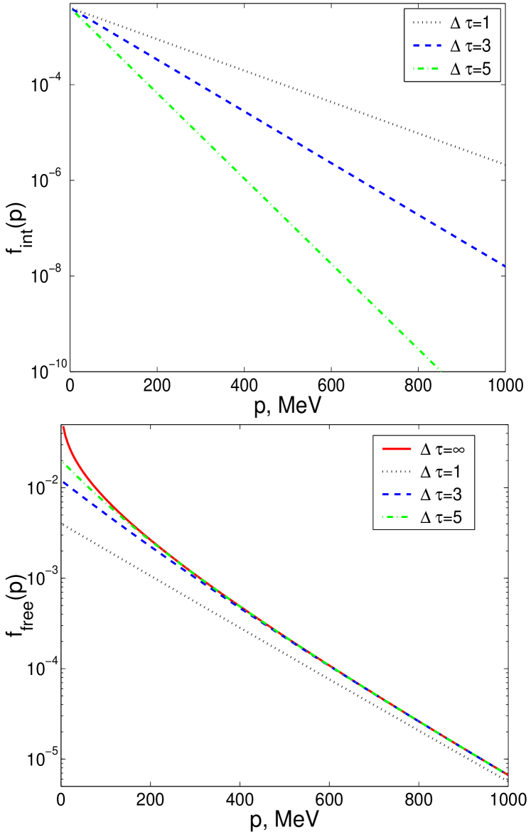
Figure 1: Figure shows the evolution of the $f_{int}$ (upper subplot) and $f_{free}$ (lower subplot) with time, $\bigtriangleup\tau=(\tau-\tau_{0})/\tau_{f}$. The initial flow velocity (which is actually kept all the time) is $v=0$, $T(\tau_{0})=170\ MeV$. We present distribution functions vs. absolute value of the momentum, since for zero flow velocity all the directions are equivalent.

2.4 Entropy condition

To obtain a physically realizable result, we have to check the condition for entropy increase:

$$S_{\tau}-S_{\tau_{0}}\geq 0\,,$$ (32)

where, for both the equilibrium and the non-equilibrium distributions the entropy current is given as

$$S^{\mu}=su^{\mu}=-\int\frac{d^{3}p}{p^{0}}\ p^{\mu}\ f(\tau)\ \left[\ln\left\{\left(2\pi\right)^{3}\ f(\tau)\right\}-1\right]\,.$$ (33)

This condition is not necessary to obtain a solution of the freeze out problem, but it should always be checked to exclude non-physical solutions.

In our case the original entropy density is given by the well known expression for the Maxwell-Boltzmann gas:

$$s(\tau_{0})=\frac{4}{3}\frac{\epsilon(\tau_{0})}{T(\tau_{0})}=\frac{4}{\pi^{2}}T^{3}(\tau_{0})\,,$$ (34)

where we have used eq. (28). The entropy density for $\tau=\infty$, when all the particles are frozen out, can be calculated through eq. (33) using the distribution function given by expression (31). We have done this integration numerically and obtained for the ratio of entropy densities:

$$R=\frac{s(\tau=\infty)}{s(\tau_{0})}=0.9449\,,$$ (35)

for any initial temperature, $T(\tau_{0})$.

Thus, we see that the entropy density is slightly decreasing during our FO process. Since we have a gradual FO this means, that in order to avoid a decrease of total entropy, our FO model has to be accompanied by an expansion, which is natural, as mentioned before, and which should lead to a volume increase by at least $6\%$ during FO. This does not sound unrealistic.

2.5 Freeze out of nucleons

Now we would like to study the situation for baryon rich matter - in this case the distribution functions will be different, since we have to take care about baryon density conservation in addition. If our system contains some nucleons in addition to pions (for simplicity we assume that there are no other mesons in the system), then the situation is the following. The EoS at the pre FO state was more complicated then eq. (24), but for the FO times it is fixed by the eq. (22). We assume that the temperature is high and the chemical potential is not too large - such that our system is pion dominated (this is reasonable assumption for ultra-relativistic heavy ion collisions). For such a system the temperature will be still basically defined by pions and we can connect $\epsilon$ and $T$ through equation (23) and correspondingly eq. (25) is also valid.

The expression for the distribution function of the interacting component now becomes (see for example Csbook ):

$$f_{int}(\tau)=\frac{1}{2\pi m^{2}TK_{2}(m/T)}\ n(\tau)e^{-\frac{p^{\mu}u_{\mu}}{T(\tau)}}\,,$$ (39)

where $m$ is the mass of the nucleon, $K_{2}(x)$ is the Bessel function of the second kind. Of course, for the proper treatment of the nucleons we would have to use Fermi statistics, but in this work we restrict ourselves to MB distributions first of all to get an analytical/semianalytical results, and secondly because MB distributions are nevertheless frequently used to fit experimental data, see for example summspectra . Since for the FO in heavy ion collisions $T\ll m$, we can use the expansion of the Bessel function:

$$K_{n}(z)|_{z\rightarrow\infty}=\sqrt{\frac{\pi}{4z}}e^{-z}\left(1+O\left({1\over z}\right)\right)\,.$$

Thus we obtain

$$f_{int}(\tau)=CT^{-3/2}(\tau)n(\tau)e^{-\frac{p^{\mu}u_{\mu}-m}{T(\tau)}}=$$

$$=C\ T^{-3/2}(\tau_{0})n(\tau_{0})e^{-{5\over 8}\frac{\tau-\tau_{0}}{\tau_{f}}}e^{-\frac{p^{\mu}u_{\mu}-m}{T(\tau_{0})e^{-\frac{\tau-\tau_{0}}{4\tau_{f}}}}}\,,$$ (40)

where $C=\frac{1}{(2m\pi)^{3/2}}$. Again we see that $f_{int}(\tau)|_{\tau\rightarrow\infty}\rightarrow 0\,.$

Now, based on the second equation in system (9), we can calculate the distribution function of the frozen out particles.

$$f_{free}(\tau)=4CT^{-3/2}(\tau_{0})n(\tau_{0})\left(p^{\mu}u_{\mu}-m\right)^{5/2}\times$$

$$\times\left[\Gamma\left(-\frac{5}{2},p^{\mu}u_{\mu}-m\right)-\Gamma\left(-\frac{5}{2},(p^{\mu}u_{\mu}-m)e^{\frac{\tau-\tau_{0}}{4\tau_{f}}}\right)\right]\,,$$ (41)

where

$$\Gamma(\alpha,x)=\int_{x}^{\infty}e^{-x}x^{\alpha-1}dx$$ (42)

is the incomplete gamma function.

$$f_{free}(\tau)|_{\tau\rightarrow\infty}\rightarrow$$

$$4CT^{-3/2}(\tau_{0})n(\tau_{0})\left(p^{\mu}u_{\mu}-m\right)^{5/2}\Gamma\left(-\frac{5}{2},p^{\mu}u_{\mu}-m\right)\,.$$ (43)

The nucleon distribution functions are presented in Figure 2. We choose the initial baryon density much smaller than normal nuclear density, $n(\tau_{0})=0.0025\ fm^{-3}$, to justify our approach Csbook –

$$\mu(\tau_{0})=T(\tau_{0})\ln\left(\left(\frac{2\pi}{mT(\tau_{0})}\right)^{3/2}ne^{m/T(\tau_{0}}\right)=$$

$$=31\ MeV\ll T(\tau_{0})=170\ MeV\,.$$

Again $f_{free}$ looks similar to some thermal distribution. In this case $f_{free}$ is saturating very fast - already the $f_{free}$ $(\bigtriangleup\tau=3)$ is a good approximation of the final $f_{free}(\bigtriangleup\tau=\infty)$. This is due to the fact that $f_{int}$ is freezing out much faster for baryons since, in addition to the exponentially decreasing temperature, it now has the baryon density, $n(\tau)$, in front, which drops down even faster than $T$.

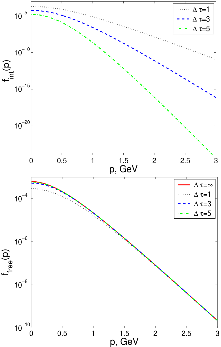
Figure 2: The same as Fig. 1, but for the nucleon distribution functions. Calculations are done for $n(\tau_{0})=0.0025\ fm^{-3}$.

3 Freeze Out of dynamically expanding system

As it was shown in section 2.4 we have to apply our FO model to the expanding system, what is natural in heavy ion collisions. The simplest, but still nontrivial, choice we kept in mind from the very beginning is the Bjorken hydrodynamical model.

Combination of this FO scenario with Bjorken scenario is straightforward. Let us, for example, concentrate on the energy density. The initial state is given at some $\tau_{in}$: $\epsilon=\epsilon(\tau_{in})$. From this moment energy density can be calculated in the Bjorken hydrodynamical model from the equation:

$$\frac{\partial\epsilon}{\partial\tau}=-\frac{\epsilon+p}{\tau}\,.$$ (44)

For the ideal ultra-relativistic gas with EoS $p=\epsilon/3$ we obtain:

$$\epsilon(\tau)=\epsilon(\tau_{in})\left(\frac{\tau_{in}}{\tau}\right)^{4/3}\,.$$ (45)

Eq. (45) is valid until moment $\tau=\tau_{0}$, when FO starts. Then during FO process energy density is given by the expression:

$$\epsilon(\tau)=\epsilon(\tau_{0})e^{-\frac{\tau-\tau_{0}}{\tau_{f}}}=\epsilon(\tau_{in})\left(\frac{\tau_{in}}{\tau_{0}}\right)^{4/3}e^{-\frac{\tau-\tau_{0}}{\tau_{f}}}\,.$$ (46)

4 Conclusions

Our analysis shows that, although the thermal post FO distributions are not restricted by general theory for the FO hypersurface with time-like normal vector, it may be too optimistic to fit particle spectra with thermal distributions. In our simple kinetic models we are able to calculate post FO distributions analytically, and we may indeed reproduce thermal post FO distribution, but only in highly simplified situation. If we take into account rescattering and consequently re-thermalization in the interacting component, the post FO distribution gets a more complicated, non-thermal form. The resulting particle distributions are in qualitative agreement with the experimentally measured pions spectra.

To clarify the principal place of our work in the field we shall make a comparison with the cut Jüttner approach of Bugaev Bu96 , eq. 5, which is the only other post FO distribution published up to recently, which satisfies the FO requirements for space-like FO surfaces. Afterwards, Bugaev’s approach was improved for space-like surfaces in Refs. FO1 ; FO3 and in subsequent publications by this research group. The present work completes this improvement work and extends it to time-like FO hypersurfaces also. Thus, more precisely, this approach is an improvement compared to Ref. Bu96 just as the works FO1 ; FO3 . This work actually completes the approach introduced in FO1 ; FO3 by extending them to time-like freeze-out surfaces. The approach is not the best of all possible approaches, it includes a few simplifying assumptions for the more transparent presentation, but it is an important advance compared to the cut Jüttner approach.

Another important point one can learn from our study is that although our post FO distribution functions are analytically very different from the Jüttner distribution, they do look pretty much like thermal distributions in some range of their parameters. Thus, observed spectra may easily be misinterpreted.

References

- (1) Josef Sollfrank et al., Phys. Rev. C 55, (1997) 392.
- (2) U. Ornik, M. Pluemer, B.R. Schlei, D. Strottman, R. M. Weiner Phys. Rev. C 54, (1996) 1381.
- (3) P.F. Kolb, J. Sollfrank, U. Heinz, Phys. Rev. C 62, (2000) 054909.
- (4) P.F. Kolb, P.Huovinen, U. Heinz, H. Heiselberg, Phys. Lett B500, (2001) 232.
- (5) P. Huovinen, P.F. Kolb, U. Heinz, H. Heiselberg, Phys. Lett B503, (2001) 58.
- (6) D. Teaney, J. Lauret, and E.V. Shuryak, Phys. Rev. Lett. 86,(2001) 4783 .
- (7) D. Molnar and M. Gyulassy, nucl-th/0104073.
- (8) M. Bleicher and H. Stocker, hep-ph/0006147.
- (9) L.V. Bravina, I.N. Mishustin, N.S. Amelin, J.P. Bondorf and L.P. Csernai, Phys. Lett. B354, (1995) 196.
- (10) L.V. Bravina, I.N. Mishustin, J.P. Bondorf and L.P. Csernai, Heavy Ion Phys. 5, (1997) 455.
- (11) H.W. Barz, L.P. Csernai and W. Greiner, Phys. Rev. C 26, (1982) 740.
- (12) F. Grassi, Y. Hama and T. Kodama, Phys. Lett. B 355, (1995) 9.
- (13) F. Grassi, Y. Hama and T. Kodama, Z. Phys. C 73, (1996) 153.
- (14) F. Grassi, Y. Hama, T. Kodama and O. Socolowski, Heavy Ion Phys. 5, (1997) 417.
- (15) H. Heiselberg, Heavy Ion Phys. 5, (1997) 435.
- (16) A.H. Taub, Phys. Rev. 74, (1948) 328.
- (17) L.P. Csernai, Sov. JETP 65, (1987) 216; Zh. Eksp. Theor. Fiz. 92, (1987) 379.
- (18) F. Cooper and G. Frye, Phys. Rev. D 10, (1974) 186.
- (19) K.A. Bugaev, Nucl. Phys. A606, (1996) 559.
- (20) Cs. Anderlik, L.P. Csernai, F. Grassi, W. Greiner, Y. Hama, T. Kodama, Zs. Lazar, V. Magas and H. Stöcker, Phys. Rev. C 59, (1999) 3309.
- (21) Cs. Anderlik, Z.I. Lázár, V.K. Magas, L.P. Csernai, H. Stöcker and W. Greiner, Phys. Rev. C 59, (1999) 388.
- (22) V.K. Magas, Cs. Anderlik, L.P. Csernai, F. Grassi, W. Greiner, Y. Hama, T. Kodama, Zs. Lázár and H. Stöcker, Heavy Ion Phys. 9, (1999) 193.
- (23) Cs. Anderlik, L.P. Csernai, F. Grassi, W. Greiner, Y. Hama, T. Kodama, Zs. Lazar, V. Magas and H. Stöcker, Phys. Lett. B459, (1999) 33.
- (24) V.K. Magas, Cs. Anderlik, L.P. Csernai, F. Grassi, W. Greiner, Y. Hama, T. Kodama, Zs. Lázár and H. Stöcker, Nucl. Phys. A661, (1999) 596.
- (25) K.A. Bugaev and M.I. Gorenstein, nucl-th/9903072.
- (26) K.A. Bugaev, nucl-th/0210087.
- (27) Yu.M. Sinyukov, Sov. Nucl. Phys. 50, (1989) 228; and Z. Phys. C 43, (1989) 401.
- (28) F. Jüttner, Ann. Physik u. Chemie 34, (1911) 865.
-
(29)
SPS data:
Nu Xu, et al., (NA44), Nucl. Phys. A 610, (1997) 175;
P.G. Jones, et al., (NA49), Nucl. Phys. A 610, (1997) 188;
RHIC data:
T. Chujo et al., (PHENIX), nucl-ex/0209027;
C. Roland et al., (PHOBOS), nucl-ex/0212006. - (30) T. Ullrich, nucl-ex/0211004.
- (31) L.P. Csernai: Introduction to Relativistic Heavy Ion Collisions (Wiley, 1994) pp. 61-63.