Genuine collective flow from Lee-Yang zeroes

Abstract

We propose to use Lee-Yang theory of phase transitions as a practical tool to analyze experimentally anisotropic flow in nucleus-nucleus collisions. We argue that this method is more reliable than any other method, and that it is the natural way to analyze collective effects.

Fifty years ago, Yang and Lee Yang:be showed that phase transitions can be characterized by the locations of the zeroes of the grand partition function in the complex plane. Since then, their theory has been extensively used, in particular, to study phase transitions in finite-size systems, via numerical simulations Chen : in lattice calculations, it has been applied to the electroweak Csikor:1998eu and QCD phase transitions Fodor:2001au .

In this Letter, we propose to apply Lee-Yang theory for the first time to the analysis of experimental data. More specifically, we show that it is the most natural way to study anisotropic flow in nucleus-nucleus collisions. Anisotropic flow is defined as a correlation between the azimuthal angle $\phi$ of an outgoing particle and the azimuthal angle $\Phi_{R}$ of the impact parameter (see Fig. 1; $\Phi_{R}$ is also called the orientation of the reaction plane), which is best characterized by the Fourier coefficients of the single-particle distribution Voloshin:1996mz :

$$v_{n}\equiv\left\langle\cos n(\phi-\Phi_{R})\right\rangle.$$ (1)

In this expression, $n$ is a positive integer and angular brackets denote an average over many particles belonging to some phase-space region, and over many collisions having approximately the same impact parameter. In particular, the so-called elliptic flow Ollitrault:bk $v_{2}$ is a sensitive probe of the dense matter produced in a nucleus-nucleus collision at ultrarelativistic energies Ackermann:2000tr .

While $v_{n}$, defined by Eq. (1), is a trivial one-particle observable which can easily be computed in a model or an event generator, the experimental situation is quite different. Indeed, the reference direction $\Phi_{R}$ is unknown experimentally, and $v_{n}$ can only be measured indirectly, from the azimuthal correlations between the detected particles. Furthermore, $\Phi_{R}$ varies randomly from one event to the other, which has a remarkable consequence: anisotropic flow appears as a truly collective motion, in the sense that all outgoing particles in a given event seem to be attracted towards some arbitrary direction.

The standard method for analyzing anisotropic flow is to correlate particles with an estimate of $\Phi_{R}$ Danielewicz:hn . However, this estimate is itself obtained from the outgoing particles, and one essentially measures a two-particle correlation Wang:1991qh . Intuitively, two-body correlations are not the appropriate tool to probe collective behaviour. Indeed, these two-particle methods were shown to be inadequate due to various “nonflow” correlations from quantum statistics Dinh:1999mn , resonance decays, minijet production Kovchegov:2002nf , etc., which are neglected and bias the analysis. Recently, new methods were developed, based on higher-order (typically, four-particle) correlations, together with a cumulant expansion which eliminates low-order nonflow correlations Borghini:2000sa . However, it was argued that experimental results Adler:2002pu could still be biased by nonflow effects Kovchegov:2002cd at this order. In this paper, $v_{n}$ will be analyzed directly from the correlation between a large number of particles. It will be shown that the results are perfectly stable with respect to nonflow correlations, which involve a smaller number of particles.

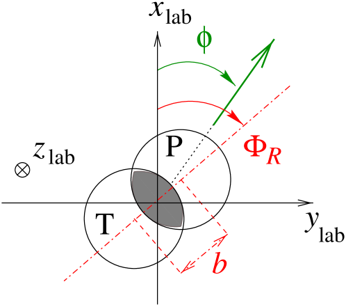
Figure 1: Schematic picture of a nucleus-nucleus collision viewed in the plane transverse to the collision axis $z$. $b$ is the impact parameter, $\Phi_{R}$ its azimuthal angle. $\phi$ is the azimuthal angle of an outgoing particle.

Our new method is based on the following global observable, which is defined for each event:

$$Q^{\theta}=\sum_{j=1}^{M}\cos n(\phi_{j}-\theta),$$ (2)

where $n$ is the Fourier harmonic under study ($n=1$ for directed flow $v_{1}$, $n=2$ for elliptic flow), the sum runs over all $M$ detected particles, $\phi_{j}$ are their azimuthal angles, and $\theta$ is an arbitrary reference direction. This quantity is nothing but a projection of the “event flow-vector,” used in other methods to estimate the orientation of the reaction plane Danielewicz:hn , on the transverse direction making an angle $n\theta$ with respect to the $x$-axis. In practice, the sum in Eq. (2) is often weighted: weights depending on the particle mass, transverse momentum and rapidity are used in order to reduce statistical errors and increase the flow signal. They are omitted here for the sake of simplicity, but should be included in the actual analysis.

The central object in the method is the moment generating function vanKampen

$$G(z)\equiv\left\langle e^{zQ^{\theta}}\right\rangle,$$ (3)

where $z$ is a complex variable, and angular brackets now denote an average over a large number of events with the same impact parameter. The procedure to obtain $v_{n}$ (as will be shown below) is the following: choose a value of $\theta$; construct $Q^{\theta}$ for each event, evaluate $G({\rm i}r)$ for real, positive $r$; plot $|G({\rm i}r)|$ as a function of $r$; determine the first minimum $r_{0}$. The flow is given by $v_{n}\simeq 2.405/Mr_{0}$.

Let us now justify the procedure. We first introduce the cumulants $c_{k}$, which are defined as vanKampen

$$\ln G(z)\equiv\sum_{k=1}^{+\infty}\frac{c_{k}}{k!}z^{k}.$$ (4)

The first two terms in this power-series expansion correspond to the average value of $Q^{\theta}$, and the square of its standard deviation, respectively:

$$c_{1}=\left\langle Q^{\theta}\right\rangle,\ \ \ c_{2}=\left\langle(Q^{\theta})^{2}\right\rangle-\left\langle Q^{\theta}\right\rangle^{2}.$$ (5)

Note that $c_{1}$ vanishes by symmetry if the detector has uniform azimuthal coverage.

The order of magnitude of the cumulants differs depending on whether or not there are collective effects in the system. Since $Q^{\theta}$ is the sum of $M$ terms of order unity, and $c_{k}$ involves $(Q^{\theta})^{k}$, the naive expectation is that $c_{k}$ should be of order $M^{k}$ or, more generally, scale with $M$ like $M^{k}$. As we shall see later, this is precisely the case when anisotropic flow is present. When no collective effect is present, however, cumulants are much smaller: one can view the system as made of independent clusters of particles. $G(z)$ then factorizes into the product of the contributions of each cluster, which is converted into a sum by the logarithm. Hence $c_{k}$ scales only linearly with $M$. For particles emitted with uncorrelated, randomly distributed azimuthal angles, for instance, Eq. (5) gives $c_{2}=M/2$.

This shows that the value of $c_{k}$ for large $k$ is the natural observable to characterize collective effects: the larger $k$, the larger the contribution of collective effects, relative to other contributions, which scale like $M$. The asymptotic behaviour of $c_{k}$ for large $k$ therefore provides a cleaner separation between collective effects and few-body correlations than finite-order cumulants Borghini:2000sa . This can be easily understood physically: the cumulant $c_{k}$ essentially isolates the contribution of genuine $k$-particle correlations, by subtracting out most contributions from lower-order correlations. In order to study collective effects, which by definition involve a large number of particles, $k$ should be as large as possible.

The asymptotic behaviour of $c_{k}$ for large $k$ is determined by the radius of convergence of the power-series expansion, Eq. (4), i.e., by the singularity of $\ln G(z)$ which lies closest to the origin in the complex plane. Since $G(z)$ has no singularity, the only possible singularities of $\ln G(z)$ are the zeroes of $G(z)$. If $z_{0}$ denotes the zero closest to the origin, $c_{k}$ scales typically like $z_{0}^{-k}$ for large $k$. Therefore, if $c_{k}$ scales like $M^{k}$ (collective effects), $z_{0}$ scales like $1/M$. If there is no collective effect, $G(z)$ is the product of contributions of small clusters, and the zeroes of $G(z)$ are the zeroes of the individual contributions: $z_{0}$ does not depend on $M$.

We are now in a position to explain how our approach relates to the theory of phase transitions of Yang and Lee Yang:be . The starting point is the grand partition function:

$${\cal G}(\mu)=\sum_{N=0}^{+\infty}Z_{N}e^{\mu N/kT},$$ (6)

where $Z_{N}$ is the canonical partition function for $N$ particles at temperature $T$ in a volume $V$ (both $T$ and $V$ are fixed). Let $\mu_{c}$ denote a reference value of the chemical potential $\mu$. The probability $P_{N}$ to have $N$ particles in the system at $\mu=\mu_{c}$ is

$$P_{N}\equiv\frac{Z_{N}e^{\mu_{c}N/kT}}{{\cal G}(\mu_{c})}.$$ (7)

The moment generating function of this probability distribution can be simply expressed in terms of the grand partition function, Eq. (6)

$$G(z)\equiv\sum_{N=0}^{+\infty}P_{N}e^{zN}=\frac{{\cal G}(\mu_{c}+kTz)}{{\cal G}(\mu_{c})}.$$ (8)

This function is analogous to our generating function, Eq. (3), with the number of particles $N$ instead of $Q^{\theta}$, and the volume $V$ instead of the multiplicity $M$. We can repeat the previous discussions: if particles are correlated only within small clusters, $z_{0}$ (the zero of $G(z)$ closest to the origin) is independent of $V$. This is the case when no phase transition occurs at $\mu=\mu_{c}$. Now assume that a first-order transition, say, a liquid-gas transition, occurs at $\mu=\mu_{c}$. Then, the system can be any mixture of the low-density gas phase and the high-density liquid phase. The probability distribution $P_{N}$ in Eq. (8) is widely spread between two values $N_{\rm min}$ (gas) and $N_{\rm max}$ (liquid) which both scale like the volume $V$. Then, the partition function $G(z)$ depends on the volume $V$ essentially through the combination $zV$, and consequently its zeroes scale with the volume like $1/V$. The general result of Lee and Yang is precisely that a phase transition occurs at $\mu=\mu_{c}$ if the zeroes of $G(z)$ come closer and closer to the origin $z=0$ as the volume of the system, $V$, increases (note, however, that Ref. Yang:be is written in terms of the variable $y=e^{z}$ instead of $z$).

Let us come back to heavy ion collisions. So far, our analysis has been general, and $Q^{\theta}$ could be replaced by any extensive variable in Eq. (3). We are now going to specify what happens when there is anisotropic flow in the system. We can repeat the discussion of Eqs. (3-5), but with all average values taken for a fixed orientation of the reaction plane $\Phi_{R}$. Such averages will be denoted by $\left\langle\cdots|\Phi_{R}\right\rangle$. Using the definition of $v_{n}$, Eq. (1), and symmetry with respect to the reaction plane (which implies $\langle\sin n(\phi-\Phi_{R})\rangle=0$), and assuming for simplicity that the multiplicity $M$ is the same for all events, one obtains from Eq. (2):

$$c_{1}=\left\langle Q^{\theta}|\Phi_{R}\right\rangle=Mv_{n}\,\cos(n(\Phi_{R}-\theta)).$$ (9)

We neglect terms $c_{3}$ and higher in Eq. (4). This amounts to assuming that the probability distribution of $Q^{\theta}$ is gaussian for a fixed $\Phi_{R}$: this is the central limit theorem, which holds if $M$ is large enough, and if there is no other collective effect in the system. We further neglect the $\Phi_{R}$-dependence of $c_{2}$. Finally, averaging over $\Phi_{R}$, one obtains the following theoretical expression of $G(z)$, which we denote by $G_{\rm c.l.}(z)$ since it corresponds to the central limit approximation:

$$G_{\rm c.l.}(z)=e^{c_{2}z^{2}/2}\,I_{0}(Mv_{n}z),$$ (10)

where $I_{0}$ is a modified Bessel function. Taking the logarithm and expanding in powers of $z$, one checks that the cumulant $c_{k}$ in Eq.(4) scales with $M$ like $M^{k}$, as anticipated.

The first zeroes of $G_{\rm c.l.}(z)$ lie on the imaginary axis at

$$z_{0}={\rm i}r_{0}=\frac{{\rm i}j_{01}}{Mv_{n}},$$ (11)

and at $-z_{0}$, where $j_{01}\simeq 2.405$ is the first positive root of the Bessel function $J_{0}(x)$. As expected from the general discussion above, anisotropic flow $v_{n}$, being a collective effect, is completely determined by $z_{0}$. The situation is analogous to a first-order phase transition, in the sense that the position of the zero scales like $1/M$, and the multiplicity $M$ is the analogue of the volume $V$ in Lee-Yang’s theory. The important difference with statistical physics is that the system size is much smaller. As a consequence, zeroes never come very close to the origin, but the physics involved is essentially the same.

In a second paper Lee:1952ig , Lee and Yang further showed that all zeroes lie on the imaginary axis of the variable $z$ (or, equivalently, on the unit circle for $y=e^{z}$) for a general class of models. It is interesting to note that our theoretical estimate, Eq. (10), has the same property.

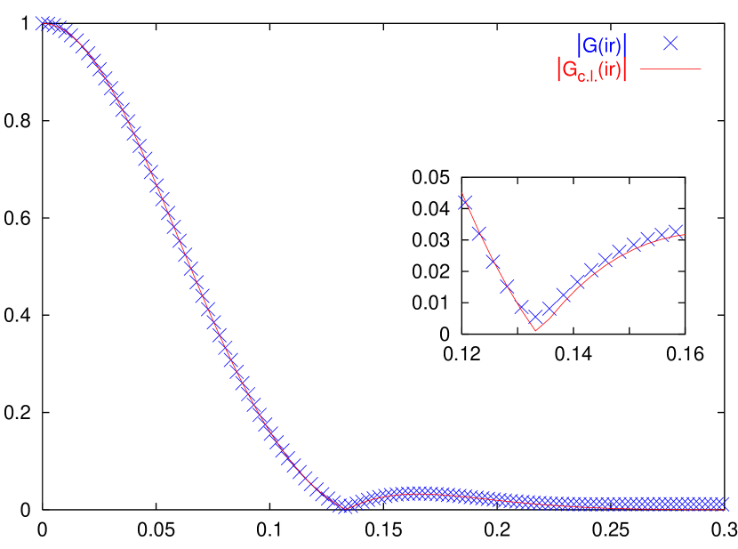
Figure 2: Variation of $\left|G(ir)\right|$ with $r$. The crosses are the values of $|G({\rm i}r)|$. The solid line displays the expected value $|G_{\rm c.l.}({\rm i}r)|$ defined by Eq. (10).

Figure 2 displays the variation of $\left|G({\rm i}r)\right|$ as a function of $r$ for simulated data. The data set contained $N_{\rm evts}=20000$ events. In each event, $M=300$ particles are emitted independently with an azimuthal distribution $dN/d\phi\propto 1+2v_{2}\cos(2(\phi-\Phi_{R}))$, where $v_{2}=6\%$, and the azimuth of the reaction plane, $\Phi_{R}$, is randomly chosen. These numbers are typical values for a mid-central Au+Au collision at $\sqrt{s_{{}_{\rm NN}}}=130$ GeV, as analyzed by the STAR Collaboration Ackermann:2000tr . The global observable $Q^{\theta}$ in Eq. (2) was constructed for each event with $n=2$ and various values of $\theta$. Figure 2 corresponds to $\theta=0$. The numerical results are compared with the theoretical estimate, Eq. (10), where we have taken $c_{2}=M/2$ (the expected value for independent particles). The excellent agreement justifies the approximations made in deriving Eq. (10). However, a closer look at the numerical results (inlay in Fig. 2) shows that unlike the theoretical estimate, $|G({\rm i}r)|$ does not strictly vanish: due to statistical fluctuations, the zeroes of $G(z)$ are slightly off the imaginary axis. This small deviation is physically irrelevant, and we choose to investigate the minima of $|G(z)|$, rather than the zeroes of $G(z)$. We denote by $r_{0}^{\theta}$ the first minimum of $|G({\rm i}r)|$, where the superscript $\theta$ recalls that it may depend on the reference angle $\theta$ in Eq. (2). Identifying $G(z)$ with the theoretical estimate $G_{\rm c.l.}(z)$, and using Eq. (11), we obtain the following estimate of $v_{n}$, which may also depend on $\theta$:

$$v_{n}^{\theta}\equiv\frac{j_{01}}{Mr_{0}^{\theta}}.$$ (12)

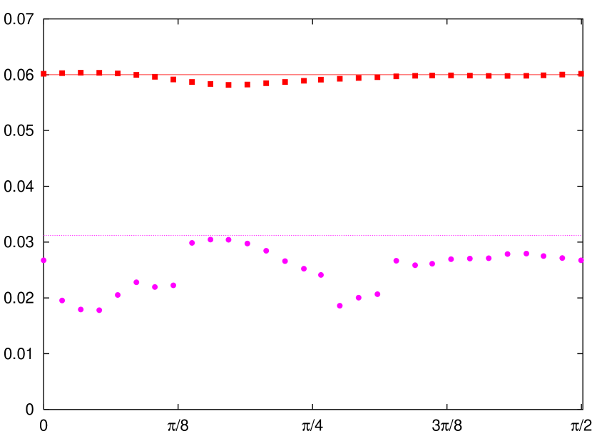
Figure 3: The reconstructed value $v_{2}^{\theta}$ as a function of $\theta$. Squares: simulated data with input $v_{2}=6\%$ (same data as in Fig. 2). Circles: simulated data with input $v_{2}=0$.

This procedure was applied to the simulated data. The result is shown in Fig. 3. $v_{2}^{\theta}$ coincides with the input value $v_{2}=6\%$, up to statistical fluctuations. Performing the analysis for several values of $\theta$, and averaging $v_{2}^{\theta}$ over $\theta$, reduces this statistical error. We finally obtain $5.95\%$: $v_{2}$ is reconstructed with great accuracy.

For the sake of illustration, we also applied the same procedure to simulated data with no flow. The procedure yields a spurious flow, due to statistical fluctuations, which is also shown in Fig. 3. The magnitude of this spurious flow can easily be understood. The average in Eq. (3) is evaluated over a finite number of events, $N_{\rm evts}$. As a consequence, $G({\rm i}r)$ has statistical fluctuations, whose typical magnitude is $1/\sqrt{N_{\rm evts}}$. For large enough $r$, they become as large as the expectation value given by Eq. (10), in which we set $v_{n}=0$ and $c_{2}=M/2$. This occurs when

$$e^{-Mr^{2}/4}\sim\frac{1}{\sqrt{N_{\rm evts}}}.$$ (13)

As soon as $r$ is larger than this value, fluctuations can produce a minimum of $|G({\rm i}r)|$. The corresponding “spurious flow” given by the analysis, Eq. (12), satisfies

$$v_{n}^{\theta}\lesssim\frac{j_{01}}{\sqrt{2M\ln N_{\rm evts}}}.$$ (14)

For our simulated data, the right-hand side (rhs) is about $3.1\%$, which is depicted as the dashed line in Fig. 3. As expected, the values of $v_{2}^{\theta}$ lie below this value, but only slightly. This is the main limitation of our method: $v_{n}$ can be safely reconstructed only if it is larger than the rhs of Eq. (14).

Since no “nonflow” correlation between the particles was simulated, standard methods of flow analysis would have worked well too. However, the unique feature of the present method is its absolute stability with respect to such correlations. As an illustration, assume that instead of emitting $M$ particles in each event, we emit $M$ clusters, each cluster containing $q$ collinear particles. Then, $Q^{\theta}$ is increased by a factor of $q$. As a consequence, the position of the first minimum, $r_{0}^{\theta}$, is smaller by a factor of $q$. Since the event multiplicity is now $qM$, one must replace $M$ with $qM$ in the denominator of Eq. (12), so that the flow estimate $v_{n}^{\theta}$ is strictly the same, as it should. On the other hand, estimates of $v_{2}$ from 2-particle or 4-particle methods Borghini:2000sa are generally increased by such correlations. With the numerical values above, the increase would be significant for 2-particle methods (one obtains $v_{2}=7.3\%$ instead of $6\%$), but very small for 4-particle cumulants: in most cases of interest, these cumulants will give results very similar to those obtained with the present method, but the latter is the most systematic one to disentangle collective motion from other effects.

The method can be extended to the analysis of differential flow, i.e., the analysis of $v_{n}$ as a function of transverse momentum and rapidity. This is explained in detail in Ref. bbo , where we also discuss in detail errors due to nonflow correlations, statistical fluctuations, and show that the method is remarkably insensitive to azimuthal asymmetries in the detector acceptance.

We have shown that Lee-Yang theory of phase transitions can be used as a practical means of analyzing anisotropic flow experimentally. The method is expected to give results similar to cumulant methods, but is significantly simpler to implement, and formally elegant. It does not require the knowledge of the reaction plane and there is no need to construct correlation functions and cumulants. More generally, Lee-Yang zeroes provide a natural probe of collective behaviour. It would be interesting to extend the present approach to other observables, in order to look for critical fluctuations which may occur in the vicinity of a phase transition. Jeon:2003gk

References

- (1) C. N. Yang, T. D. Lee, Phys. Rev. 87 (1952) 404.
- (2) C.-N. Chen, C.-K. Hu, F. Y. Wu, Phys. Rev. Lett. 76 (1996) 169.
- (3) F. Csikor, Z. Fodor, J. Heitger, Phys. Rev. Lett. 82 (1999) 21.
- (4) Z. Fodor, S. D. Katz, Phys. Lett. B 534 (2002) 87.
- (5) T. C. Brooks, K. L. Kowalski, C. C. Taylor, Phys. Rev. D 56 (1997) 5857.
- (6) S. Voloshin, Y. Zhang, Z. Phys. C 70 (1996) 665.
- (7) J.-Y. Ollitrault, Phys. Rev. D 46 (1992) 229.
- (8) STAR Collaboration, K. H. Ackermann, et al., Phys. Rev. Lett. 86 (2001) 402.
- (9) P. Danielewicz, G. Odyniec, Phys. Lett. B 157 (1985) 146; A. M. Poskanzer, S. A. Voloshin, Phys. Rev. C 58 (1998) 1671.
- (10) S. Wang, et al., Phys. Rev. C 44 (1991) 1091.
- (11) P. M. Dinh, N. Borghini, J.-Y. Ollitrault, Phys. Lett. B 477 (2000) 51; N. Borghini, P. M. Dinh, J.-Y. Ollitrault, Phys. Rev. C 62 (2000) 034902.
- (12) Y. V. Kovchegov, K. L. Tuchin, Nucl. Phys. A 708 (2002) 413.
- (13) N. Borghini, P. M. Dinh, J.-Y. Ollitrault, Phys. Rev. C 63 (2001) 054906; Phys. Rev. C 64 (2001) 054901.
- (14) STAR Collaboration, C. Adler, et al., Phys. Rev. C 66 (2002) 034904.
- (15) Y. V. Kovchegov, K. L. Tuchin, Nucl. Phys. A 717 (2003) 249.
- (16) N. G. van Kampen, Stochastic Processes in Physics and Chemistry (North-Holland, Amsterdam, 1981).
- (17) T. D. Lee, C. N. Yang, Phys. Rev. 87 (1952) 410.
- (18) R. S. Bhalerao, N. Borghini, J.-Y. Ollitrault, Nucl. Phys. A 727 (2003) 373.
- (19) S. Jeon, V. Koch, hep-ph/0304012.