Effect of Resonant Continuum on Pairing Correlations in the Relativistic Approach

Abstract

A proper treatment of the resonant continuum is to take account of not only the energy of the resonant state, but also its width. The effect of resonant states on pairing correlations is presented in the framework of the relativistic mean field theory plus Bardeen-Cooper-Schrieffer (BCS) approximation with a constant pairing strength. The study is performed in an effective Lagrangian with the parameter set NL3 for neutron rich even-even Ni isotopes. Results show that the contribution of the proper treatment of the resonant continuum to pairing correlations for those nuclei close to neutron drip line is important. The pairing gaps, Fermi energies, pairing correlation energies, and binding energies are considerably affected with a proper consideration of the width of resonant states. The problem of unphysical particle gas, which may appear in the calculation of the traditional mean field plus BCS method for nuclei in the vicinity of drip line could be well overcome when the pairing correlation is performed by using the resonant states instead of the discretized states in the continuum.

I introduction

The study of properties of exotic nuclei, in particular the structure of nuclei far from the $\beta$-stability line, has recently attracted wide interest both experimentally and theoretically. In those nuclei, the presence of nucleons, which have separation energies appreciably smaller than those in ${\beta}$-stable nuclei and have a far extending nucleon distribution, leads to various interesting physical phenomena. Due to the closeness of the Fermi surface to the particle continuum in exotic nuclei the coupling between bound states and the continuum become important. The description of exotic nuclei has to explicitly include the coupling between bound states and the continuum. There exist several extensive studies of exotic nuclei in relativistic and non-relativistic microscopic approachesRing96 ; Dob98 ; Kuo97 ; Dob96 . A key ingredient of those models is how to properly treat the pairing correlations which have an important influence on physical properties in exotic nuclei. In general, pairing correlations in open shell nuclei can be treated by the Bardeen-Cooper-Schrieffer (BCS) theory or through the Bogoliubov transformationRing80 . The main feature of the Bogoliubov transformation, compared with the simple BCS theory, is that the Hartree-Fock equation or Dirac equation and the gap equations are solved simultaneously with self-consistent fields. Both of them could give a good description of the pairing correlation if the nucleus is not too far away from the $\beta$-stable lineLi02 . The simple BCS method may not be reliable near the drip line because the continuous states were not correctly treatedLi02 ; Dob84 . The contribution of the coupling to the continuum would be prominent when the nucleus close to the drip line, therefore a proper treatment of the continuum becomes more important. Single particle resonant states in the continuum, which differ from bound states, are metastable states with life times due to a sufficiently high centrifugal barrier (for neutrons and protons) and Coulomb barrier (for protons). The effect of the widths of resonant states on pairing correlations was not estimated by the usual non-relativistic Hartree-Fock-Bogoliubov (HFB)Dob96 ; Ring80 or the relativistic Hartree-Bogoliubov (RHB)Ring91 . The effect of a proper treatment of the resonant continuum on the pairing in the non-relativistic approach has been investigatedSan97 ; San00 ; Kru01 . The investigation in the relativistic approach is reported very recentlySan032 .

In this paper, we aim at the investigation on the effect of the resonant continuum on pairing correlations of neutron rich nuclei in the relativistic mean field theory plus BCS (RMF+BCS) approximation. Particularly we shall focus our attention on the effect of widths of single particle resonant states in the description of neutron rich nuclei. It has been pointed out that pairing correlations could be well described by the simple BCS theory if single particle states in the continuum are properly treatedSan97 ; San00 ; Kru01 . It is known that narrow resonant states in the continuum are well localized inside the nucleus due to a sufficiently high centrifugal barrier and Coulomb barrier (for proton only). In our previous workCao02 , we have shown that the nuclear dynamical processes can also be well described by the simple method where the continuum was replaced by only a few single particle resonant states. Therefore, we may expect that using a few single particle resonant states instead of the discretized continuum, the pairing space would be large enough in order to give a good description on the ground state properties of neutron rich nuclei in the RMF, even within the BCS approximation.

Usually pairing correlations in the BCS approximation are treated in a phenomenological way based on empirical pairing gaps deduced from odd-even mass differences. This procedure works well in the valley of $\beta$-stability, where experimental masses are known. The predictive power for pairing gaps for nuclei far from the $\beta$-stability line is thus limited due to the unknown masses of such nuclei. Therefore, a constant pairing strength is usually employed in the BCS calculationEst01 . We shall investigate the pairing effect in the RMF with the parameter set NL3Lal97 , which give a good description of not only the ground state propertiesLas99 but also the collective giant resonanceMa01 ; Ma02 ; Ring01 ; Cao03 . To investigate the width effect of single particle resonant states on pairing correlations, we compare the results in three types of calculations: (a) the RMF+BCS approach where quasi-particle wave functions are obtained by a box boundary condition; (b) the extended RMF+BCS approximation where wave functions of resonant states are calculated by imposing a proper scattering boundary condition for the continuous spectrum but the width of resonant states is not considered, which is denoted as RMF+BCSR; (c) the full RMF+BCS (RMF+BCSRW) calculation where widths of single particle resonant states are taken into account explicitly.

The paper is arranged as the follows. In Sec.II and Sec.III the relativistic mean field theory and the BCS approximation with explicitly considering the widths of the resonant continuum are presented. The effect of the resonant continuum on pairing correlations is formulated by introducing a continuum level density into the gap equations. The results calculated by different models mentioned above for neutron rich even-even Ni isotopes are given and discussed in Sec.IV. Finally we give a brief summary in Sec.V.

II Relativistic Mean Field Theory

The RMF theory Ring96 ; Hor81 ; Ser86 is based on the effective Lagrangian density which includes the nucleon field ($\psi$), the isoscalar scalar meson field ($\sigma$), the isoscalar vector meson field ($\omega$), the isovector vector meson field ($\rho$), and electromagnetic field ($A$). The Lagrangian density is expressed as the following:

$$\cal{L} = \overline{\psi}(i\gamma^{\mu}\partial_{\mu}-M)\psi+\frac{1}{2}\partial_{\mu}\sigma\partial^{\mu}\sigma-U(\sigma)-\frac{1}{4}\Omega_{\mu\nu}\Omega^{\mu\nu}$$ (1)

$$+\frac{1}{2}m_{\omega}^{2}\omega_{\mu}\omega^{\mu}-\frac{1}{4}{{\mbox{\boldmath$R$}}}_{\mu\nu}{{\mbox{\boldmath$R$}}}^{\mu\nu}+\frac{1}{2}m_{\rho}^{2}{{\mbox{\boldmath$\rho$}}}_{\mu}{{\mbox{\boldmath$\rho$}}}^{\mu}-\frac{1}{4}F_{\mu\nu}F^{\mu\nu}$$

$$-g_{\sigma}\overline{\psi}\sigma\psi-g_{\omega}\overline{\psi}\gamma^{\mu}\omega_{\mu}\psi-g_{\rho}\overline{\psi}\gamma^{\mu}{{\mbox{\boldmath$\rho$}}}_{\mu}\cdot{{\mbox{\boldmath$\tau$}}}\psi$$

$$-e\overline{\psi}\gamma^{\mu}A_{\mu}\left(\frac{1-\tau_{3}}{2}\right)\psi~{},$$

where $M$, $m_{\sigma}$, $m_{\omega}$, and $m_{\rho}$ denote the nucleon, $\sigma$, $\omega$, and $\rho$ mesons masses, respectively, while $g_{\sigma}$, $g_{\omega}$ and $g_{\rho}$ are the corresponding coupling constants for the mesons, respectively. The vectors in isospin space are denoted by bold-faced symbols. $\Omega^{\mu\nu}$, ${{\mbox{\boldmath$R$}}}^{\mu\nu}$ and $F^{\mu\nu}$ are the field tensors of the vector fields $\omega$, $\rho$ and of the photon, respectively, they are defined as:

$$\Omega^{\mu\nu}=\partial^{\mu}\omega^{\nu}-\partial^{\nu}\omega^{\mu}~{},$$ (2)

$${{\mbox{\boldmath$R$}}}^{\mu\nu}=\partial^{\mu}{{\mbox{\boldmath$\rho$}}}^{\nu}-\partial^{\nu}{{\mbox{\boldmath$\rho$}}}^{\mu}~{},$$ (3)

$$F^{\mu\nu}=\partial^{\mu}A^{\nu}-\partial^{\nu}A^{\mu}~{},$$ (4)

In the Eq.(1), a non-linear scalar self-interaction termBog77 $U(\sigma)$ of the $\sigma$ meson has been taken into account:

$$U(\sigma)=\frac{1}{2}m_{\sigma}^{2}\sigma^{2}+\frac{1}{3}g_{2}\sigma^{3}+\frac{1}{4}g_{3}\sigma^{4}~{},$$ (5)

The Dirac equation of a single-particle state in the RMF approximation can be expressed as following:

$$\left[{{\mbox{\boldmath$\alpha$}}}\cdot{{\mbox{\boldmath$p$}}}+V(r)+\beta\left(M-S(r)\right)\right]\psi_{\alpha}=E_{\alpha}\psi_{\alpha}~{},$$ (6)

where $E_{\alpha}$ and $\psi_{\alpha}$ are the single-particle energy and wave function, respectively. $S(r)$ and $V(r)$ are an attractive scalar and repulsive vector potential, respectively. In the RMF approximation, scalar and vector potentials are produced by the classical meson fields: isoscalar $\sigma$, $\omega$ and isovector $\rho$ mesons as well as the photon, which are obtained in a self-consistent calculation for the nuclear ground stateRing96 ; Hor81 ; Ser86 . The nucleon spinor $\psi_{\alpha}$ in the Dirac equation is expressed as:

$$\psi_{\alpha}({{\mbox{\boldmath$r$}}})=\frac{1}{r}\left(\begin{array}[]{c}iG_{a}(r)\\ F_{a}(r){{\mbox{\boldmath$\sigma$}}}\cdot{{\mbox{\boldmath$\hat{r}$}}}\end{array}\right)\Phi_{\kappa,m}(\hat{r})\chi_{\frac{1}{2}}~{},$$ (7)

where $G_{a}$ and $F_{a}$ are upper and lower components of nucleon wave function, $\chi_{\frac{1}{2}}$ is the isospinor and $\Phi_{\kappa,m}$ is a spherical harmonics function. $\alpha$ is a set of quantum numbers $\alpha=(n,l,j,m,\tau_{3})\equiv(a,m,\tau_{3})$. $\kappa$ is the Dirac quantum number given by:

$$\kappa=\left\{\begin{array}[]{lll}-(j+\frac{1}{2}),&\text{for}&j=l+\frac{1}{2}\\ +(j+\frac{1}{2}),&\text{for}&j=l-\frac{1}{2}\\ \end{array}\right.~{}.$$ (10)

For spherical nuclei, the Dirac equation can be reduced to coupled equations of the radial part for $G_{a}(r)$ and $F_{a}(r)$:

$$\frac{d}{dr}\left(\begin{array}[]{c}G_{a}(r)\\ F_{a}(r)\end{array}\right)=\left(\begin{array}[]{cc}-\frac{\kappa}{r}&M+E_{a}-S(r)-V(r))\\ M-E_{a}-S(r)+V(r)&\frac{\kappa}{r}\end{array}\right)\left(\begin{array}[]{c}G_{a}(r)\\ F_{a}(r)\end{array}\right)~{},$$ (11)

where $S(r)$ is the scalar potential:

$$S(r)=g_{\sigma}\sigma(r)~{},$$ (12)

and $V(r)$ denotes the vector potential:

$$V(r)=g_{\omega}\omega_{0}(r)+g_{\rho}\tau_{3}\rho_{0}(r)+e\frac{1-\tau_{3}}{2}A_{0}(r)~{},$$ (13)

The meson and electromagnetic fields obey the radial Laplace equations:

$$\frac{d^{2}}{dr^{2}}\sigma(r)+\frac{2}{r}\frac{d}{dr}\sigma(r)-m_{\sigma}^{2}\sigma(r)=-g_{\sigma}\rho_{s}(r)-g_{2}\sigma^{2}(r)-g_{3}\sigma^{3}(r)~{},$$ (14)

$$\frac{d^{2}}{dr^{2}}\omega_{0}(r)+\frac{2}{r}\frac{d}{dr}\omega_{0}(r)-m_{\omega}^{2}\omega_{0}(r)=-g_{\omega}\rho_{v}(r)~{},$$ (15)

$$\frac{d^{2}}{dr^{2}}\rho_{0}(r)+\frac{2}{r}\frac{d}{dr}\rho_{0}(r)-m_{\rho}^{2}\rho_{0}(r)=-g_{\rho}\rho_{3}(r)~{},$$ (16)

$$\frac{d^{2}}{dr^{2}}A_{0}(r)+\frac{2}{r}\frac{d}{dr}A_{0}(r)=-e\rho_{c}(r)~{},$$ (17)

with

$$\rho_{s}(r)=\sum_{a}^{occ}\frac{2j_{a}+1}{4\pi}(|G_{a}(r)|^{2}-|F_{a}(r)|^{2})~{},$$ (18)

$$\rho_{v}(r)=\sum_{a}^{occ}\frac{2j_{a}+1}{4\pi}(|G_{a}(r)|^{2}+|F_{a}(r)|^{2})~{},$$ (19)

$$\rho_{3}(r)=\sum_{a}^{occ}\frac{2j_{a}+1}{4\pi}\tau_{3}(|G_{a}(r)|^{2}+|F_{a}(r)|^{2})~{},$$ (20)

$$\rho_{c}(r)=\sum_{a}^{occ}\frac{2j_{a}+1}{4\pi}\left(\frac{1-\tau_{3}}{2}\right)(|G_{a}(r)|^{2}+|F_{a}(r)|^{2})~{},$$ (21)

The sums $a$ run over all occupied states. The Dirac equation Eq.(9) and the corresponding meson field functions Eq.(12 - 14) as well as the photon field function Eq.(15) with expressions for source terms (16 - 19) can be solved self-consistently. More details on the relativistic mean-field theory can be found in Refs.Ring96 ; Hor81 ; Ser86 .

III BCS Approximation with Resonant Continuum

It is well known that the pairing correlation plays an important role in describing the ground state properties of open shell nuclei. The non-relativistic HFBDob96 ; Ring80 or RHBRing91 theory can provide a unified description on the mean field and pairing correlations, but they require much more numerical effort than the simple BCS theory. However, the width effect of resonant states in the gap equation is missing in most previous works of the BCS theory or the Bogoliubov transformation. Recently, properly treating the contribution of resonant continuum to pairing correlations has been investigated in the non-relativistic HF+BCS as well as HFB in Refs.San97 ; San00 ; Kru01 ; Gra01 . It has been pointed outGra01 that the resonant continuum HF+BCS approximation with a proper treatment of resonant continuum can reproduce the pairing correlation energies predicted by the continuum HFB approach up to the drip line. In this paper, we investigate the width effect of single particle resonant states on the pairing correlations in the relativistic approach. The pairing correlations of open shell nuclei are treated based on the RMF within the BCS approximation. A constant pairing strength is adopted in the BCS theory. Although the extended RMF+BCS theory formulated with correct boundary conditions for the continuous spectrum is available in the literatureSan032 , in the following we briefly summarize the essential points together with our model. From Ref.Ring80 , assuming constant pairing matrix elements in the vicinity of Fermi level, one can obtain the so-called gap equations:

$$\sum_{a}\left(j_{a}+\frac{1}{2}\right)\frac{1}{\sqrt{(\varepsilon_{a}-\lambda)^{2}+\Delta^{2}}}=\frac{2}{G}~{},$$ (22)

$$\sum_{a}\left(j_{a}+\frac{1}{2}\right)\left[1-\frac{\varepsilon_{a}-\lambda}{\sqrt{(\varepsilon_{a}-\lambda)^{2}+\Delta^{2}}}\right]=N~{},$$ (23)

where $\lambda$, $\Delta$, and $G$ represent the Fermi energy, pairing gap, and the pairing force constant, respectively. $N$ is the number of neutrons or protons involved in the pairing correlations. The solution of those two coupled equations, Eq.(20) and (21) allows one to find $\lambda$ and $\Delta$. The contribution of the pairing interaction to the total energy can be expressed as following:

$$E_{pair}=-G\left[\sum_{a}\left(j_{a}+\frac{1}{2}\right)v_{a}u_{a}\right]^{2}~{},$$ (24)

where $v_{a}^{2}$ is the occupation probability of a state with quantum numbers $\alpha=(n,l,j,m,\tau_{3})\equiv(a,m,\tau_{3})$ and $u_{a}^{2}=1-v_{a}^{2}$. For spherical nuclei, the eigenvalues of Dirac equations are of degeneracy for magnetic quantum numbers $m$ within the same $(n,l,j)$. One has:

$$\left(\begin{array}[]{c}v_{a}^{2}\\ u_{a}^{2}\end{array}\right)=\frac{1}{2}\left(1\mp\frac{\varepsilon_{a}-\lambda}{\sqrt{(\varepsilon_{a}-\lambda)^{2}+\Delta^{2}}}\right)~{},$$ (25)

In principle, the continuous spectrum is also the solution of Dirac Eq.(9), both continuous and bound states constitute a complete set of basis. In most previous theoretical nuclear structure calculations, single particle states in the continuum are usually treated in a discretization procedure by expanding wave functions in a set of harmonic oscillator basis or setting a box. This approximation, however, can be justified for very narrow resonances and gives a global description of the contributions from the continuum. In this work we introduce single particle resonant states into the pairing gap equations instead of the discretized continuous states in order to investigate the width effect of resonances on pairing correlations. The resonant state wave function are obtained by imposing a scattering boundary condition. At the distance R where the nuclear potentials vanish, the upper component of the neutron radial wave function has the following asymptotic behavior:

$$G_{\nu}(kr)=A_{\nu}\left[j_{l_{\nu}}(kr)-\tan\delta_{\nu}n_{l_{\nu}}(kr)\right]~{},~{}~{}~{}~{}~{}{\textrm{for}}~{}~{}r\geq R~{}.$$ (26)

where $j_{l_{\nu}}$ and $n_{l_{\nu}}$ are spherical Bessel and Neumann functions, respectively, and $\delta_{\nu}$ is the phase shift corresponding to the angular momentum $(l_{\nu},j_{\nu})$, $k^{2}=E^{2}-M^{2}$. For the case of proton, the asymptotic behavior can be obtained by replacing the spherical Bessel and Neumann functions in Eq.(24) with the relativistic regular and irregular Coulomb wave functionsGre90 , respectively. The energy of a resonant state is determined when the phase shift of the scattering state reaches $\pi/2$. The wave function of scattering state is normalized to a delta function of energy $\delta(E-E^{\prime})$. This condition fixes the normalization constant $A_{\nu}$, it can be obtained as:

$$A_{\nu}=\cos\delta_{\nu}\sqrt{\frac{1}{\pi}\frac{M+E}{2k}}~{},$$ (27)

In order to take into account the width effect of resonant states in the continuum we introduce a level density of the continuumBon84 into the gap equations. When we introduce single particle resonant states with widths into the pairing correlations, the gap equations can be expressed as:

$$\sum_{a}\left(j_{a}+\frac{1}{2}\right)\frac{1}{\sqrt{(\varepsilon_{a}-\lambda)^{2}+\Delta^{2}}}+\sum_{\nu}\left(j_{\nu}+\frac{1}{2}\right)\int_{I_{\nu}}\frac{g_{\nu}(\varepsilon_{\nu})}{\sqrt{(\varepsilon_{\nu}-\lambda)^{2}+\Delta^{2}}}d\varepsilon_{\nu}=\frac{2}{G}~{},$$ (28)

$$\sum_{a}\left(j_{a}+\frac{1}{2}\right)\left[1-\frac{\varepsilon_{a}-\lambda}{\sqrt{(\varepsilon_{a}-\lambda)^{2}+\Delta^{2}}}\right]+\sum_{\nu}\left(j_{\nu}+\frac{1}{2}\right)\int_{I_{\nu}}g_{\nu}(\varepsilon_{\nu})\left[1-\frac{\varepsilon_{\nu}-\lambda}{\sqrt{(\varepsilon_{\nu}-\lambda)^{2}+\Delta^{2}}}\right]d\varepsilon_{\nu}=N~{}.$$ (29)

The sums $a$ and $\nu$ run over the bound states and resonant states involved in the pairing calculation, respectively, and $I_{\nu}$ is an energy interval associated with each partial wave $(l_{\nu},j_{\nu})$. The factor $g_{\nu}$ is defined as:

$$g_{\nu}(\varepsilon_{\nu})=\frac{1}{\pi}\frac{d\delta_{\nu}}{d\varepsilon_{\nu}}~{},$$ (30)

which is the so-called continuum level density and $\delta_{\nu}$ is the phase shift of the scattering state with angular momentum $\nu=(l_{\nu},j_{\nu})$. The factor $g_{\nu}$ represents the variation of the localization of scattering states in the energy region of a resonance, in other words, it reflects the widths effect of the resonant states. For a very narrow resonant state, the factor $g_{\nu}$ becomes a delta function.

Taking account of those resonant continuum in the gap equations, the expressions of various densities in Eq.(16 - 19) have to be modified. They can be expressed as:

$$\rho_{s}(r) = \sum_{a}\frac{2j_{a}+1}{4\pi}v_{a}^{2}(|G_{a}(r)|^{2}-|F_{a}(r)|^{2})$$ (31)

$$+\sum_{\nu}\frac{2j_{\nu}+1}{4\pi}\int_{I_{\nu}}(|G_{\nu}(r)|^{2}-|F_{\nu}(r)|^{2})g_{\nu}(\varepsilon_{\nu})v_{\nu}^{2}(\varepsilon_{\nu})d\varepsilon_{\nu}~{},$$

$$\rho_{v}(r) = \sum_{a}\frac{2j_{a}+1}{4\pi}v_{a}^{2}(|G_{a}(r)|^{2}+|F_{a}(r)|^{2})$$ (32)

$$+\sum_{\nu}\frac{2j_{\nu}+1}{4\pi}\int_{I_{\nu}}(|G_{\nu}(r)|^{2}+|F_{\nu}(r)|^{2})g_{\nu}(\varepsilon_{\nu})v_{\nu}^{2}(\varepsilon_{\nu})d\varepsilon_{\nu}~{},$$

$$\rho_{3}(r) = \sum_{a}\frac{2j_{a}+1}{4\pi}\tau_{3}v_{a}^{2}(|G_{a}(r)|^{2}+|F_{a}(r)|^{2})$$ (33)

$$+\sum_{\nu}\frac{2j_{\nu}+1}{4\pi}\tau_{3}\int_{I_{\nu}}(|G_{\nu}(r)|^{2}+|F_{\nu}(r)|^{2})g_{\nu}(\varepsilon_{\nu})v_{\nu}^{2}(\varepsilon_{\nu})d\varepsilon_{\nu}~{},$$

$$\rho_{c}(r) = \sum_{a}\frac{2j_{a}+1}{4\pi}\left(\frac{1-\tau_{3}}{2}\right)v_{a}^{2}(|G_{a}(r)|^{2}+|F_{a}(r)|^{2})$$ (34)

$$+\sum_{\nu}\frac{2j_{\nu}+1}{4\pi}\left(\frac{1-\tau_{3}}{2}\right)\int_{I_{\nu}}(|G_{\nu}(r)|^{2}+|F_{\nu}(r)|^{2})g_{\nu}(\varepsilon_{\nu})v_{\nu}^{2}(\varepsilon_{\nu})d\varepsilon_{\nu}~{},$$

The Dirac equation Eq.(9) and meson field functions (12 - 14) as well as the photon field function (15) with corresponding densities (29 - 32) are solved self-consistently in an iterative way. Therefore, the total binding energy can be written as:

$$E = \sum_{a}\left(2j_{a}+1\right)v_{a}^{2}E_{a}+\sum_{\nu}\left(2j_{\nu}+1\right)\int_{I_{\nu}}g_{\nu}(\varepsilon_{\nu})v_{\nu}^{2}(\varepsilon_{\nu})\varepsilon_{\nu}d\varepsilon_{\nu}$$ (35)

$$-\frac{1}{2}\int\left(g_{\sigma}\rho_{s}\sigma_{0}+g_{\omega}\rho_{\nu}\omega_{0}+g_{\rho}\rho_{3}\rho^{3}_{0}+e\rho_{c}A_{0}\right)d^{3}r$$

$$-\int\left(\frac{1}{3}g_{2}\sigma_{0}^{3}+\frac{1}{4}g_{3}\sigma_{0}^{4}\right)d^{3}r$$

$$-G\left[\sum_{a}\left(j_{a}+\frac{1}{2}\right)v_{a}u_{a}+\sum_{\nu}\left(j_{\nu}+\frac{1}{2}\right)\int_{I_{\nu}}g_{\nu}(\varepsilon_{\nu})v_{\nu}(\varepsilon_{\nu})u_{\nu}(\varepsilon_{\nu})d\varepsilon_{\nu}\right]^{2}$$

$$-\frac{3}{4}\cdot 41\cdot A^{-1/3}~{},$$

Where the last two terms are the pairing energy and the correction for the spurious center of mass motion, respectively.

IV Properties of neutron rich even-even Ni isotopes

In this work we investigate the ground state properties of neutron rich even-even Ni isotopes in the RMF+BCS model and explicitly take account of the continuum. Particularly we shall focus our attention on the effect of single particle resonant states on the pairing correlation in those neutron rich nuclei. Calculations are carried out in the RMF with the parameter set NL3. Three types of calculations: RMF+BCS, RMF+BCSR and RMF+BCSRW are performed. The effect of single particle states in the continuum on the ground state properties is investigated.

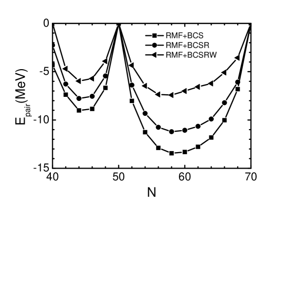
Figure 1: The pairing energies for neutron rich even-even Ni isotopes with $N=40-70$. The solid squares, circles and left-triangles denote the results calculated in the RMF+BCS, RMF+BCSR and RMF+BCSRW approaches, respectively. All calculations are performed with the parameter set NL3.

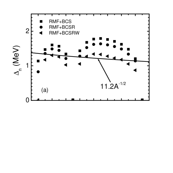
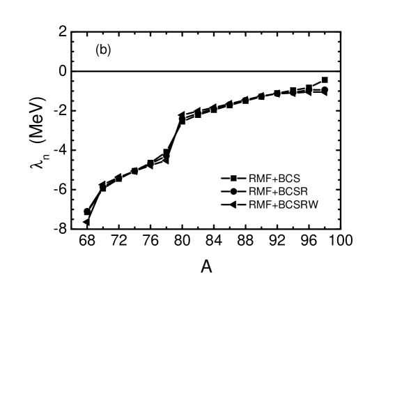
Figure 2: The neutron pairing gap (a) and Fermi energy (b) as a function of the atomic number $A$. The notations are same as in Fig.1.

In our investigation, the proton number of Ni isotopes is $Z=28$, which is a closed shell. Therefore, the proton pairing gap is taken to be zero. For the neutron case, we use a state-independent pairing strength $G=C/A$, where the constant $C=20.5$ MeV is adopted from Ref.Est01 . It could also provide a best fit to reproduce experimental binding energies of known Ni-isotopes. In practical calculations, we restrict the pairing space to about one harmonic oscillator shell above and below the Fermi surface in the RMF+BCS model. The levels include $1f_{5/2}$, $2p_{3/2}$, $2p_{1/2}$,$1g_{9/2}$, $2d_{5/2}$, $3s_{1/2}$, $2d_{3/2}$, $1g_{7/2}$, $1h_{11/2}$ and $2f_{7/2}$, some of them, such as $2d_{5/2},~{}2d_{3/2},~{}1g_{7/2},~{}2f_{7/2}$, and $1h_{11/2}$ are single particle resonant states, depending on the isotopes. Highly excited resonant states with large widths, such as $1h_{9/2}$ and $1i_{13/2}$, are ignored in our calculations. Obviously, an enlarged pairing space in the normal BCS calculation would change the pairing contribution due to a constant pairing interaction. Therefore the results in cases of RMF+BCS and RMF+BCSR in Fig.1 and Fig.2 would be different if one includes more states in the pairing active space. It is found that the pairing properties are not affected too much if one includes the resonant states $1h_{9/2}$ and $1i_{13/2}$ with wide widths in the RMF+BCSRW calculation.

The single particle energies and wave functions are first carried out by solving the Dirac equation Eq.(9) self-consistently. Using those single particle states we can solve the BCS gap equations in the three approaches. The Fermi energy and gap as well as the occupation probabilities of quasi-particle states are obtained simultaneously. The nuclear densities composed of quasi-particle states and potentials are recalculated. Then we solve Dirac equation again by an iterative way until the convergence is reached. The pairing correlation energies can be obtained in the Eq.(22) in the three approaches, which are shown in Fig.1 for neutron rich even-even Ni isotopes of $N=40$ to 70. Pronounced differences of the pairing energies performed in various RMF+BCS approaches are observed for open shell nuclei, where the behavior of pairing energies is similar to those obtained by the RHB in Refs.Meng98 . The usual RMF+BCS approach produces the largest pairing energies, due to some non-resonant scattering states in the continuum are included. It can be seen in Fig.1 that the pairing energies are reduced largely when the widths of single particle resonant states are taken into account in the RMF+BCSRW calculation.

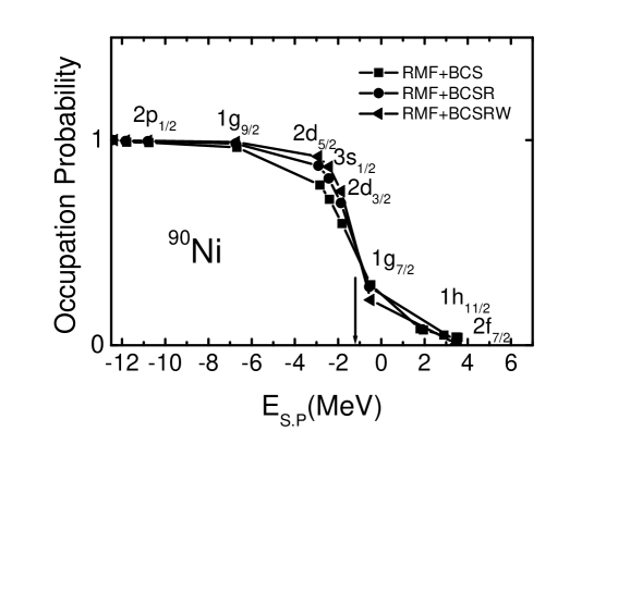
Figure 3: The occupation probabilities for ⁹⁰Ni as a function of the single particle energy around the threshold. The results are performed in RMF+BCS, RMF+BCSR and RMF+BCSRW approaches with the effective nonlinear interaction NL3. The notations are same as in Fig.1.

In order to understand the difference presented by different treatments on pairing correlations, we plot the results of pairing gaps and Fermi energies for neutron rich even-even Ni isotopes with masses from 68 to 98 in Fig.2(a) and Fig.2(b). The curve in Fig.2 (a) is the empirical pairing gap given by $11.2/\sqrt{A}$. It is observed that pairing gaps are largely decreased when the width effect of single particle resonant states is taken in account in pairing correlation calculations, while the Fermi energies remain unchanged for three approaches. This feature agrees with the case in the non-relativistic HF+BCS calculationsSan00 . It is found that the pairing gaps in the RMF+BCSR calculation are close to those obtained in the box RMF+BCS approximation. As an example, for the neutron rich nucleus ⁹⁰Ni, the pairing gap and Fermi energy are $\Delta_{n}$ =1.558 MeV and $\lambda_{n}$=-1.278 MeV in the RMF+BCSR approach, whereas, they are reduced to 1.223 MeV and -1.256 MeV, respectively when we perform the pairing correlation calculations by considering the width effect of resonances explicitly. The reduced pairing gap and Fermi energy could change the occupation probability of neutrons at each single particle orbit near the Fermi surface. In Fig.3 we show the occupation probabilities of neutron single particle levels in ⁹⁰Ni as a function of corresponding energies. The arrow is the position of the neutron Fermi surface. In ⁹⁰Ni the Fermi energy is very close to the continuum, therefore the continuum becomes important in the pairing correlations. Some scattering states in the continuum, such as states 3$p_{3/2}$ and 3$p_{1/2}$, which are not resonance states due to the low centrifugal barrier, are included in the RMF+BCS calculation. Therefore the RMF+BCS approach overestimates the pairing correlation and produces large pairing energies and pairing gaps. It is found that the width effect on the pairing is to reduce the pairing correlations, therefore occupation probabilities of low-lying states below the Fermi surface in the case of RMF+BCSRW are slightly larger than those without the width effect, and vice versa for states above Fermi surface.

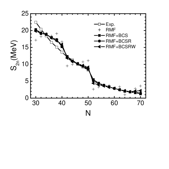
Figure 4: Two-neutron separation energies for neutron rich even-even Ni isotopes calculated in the RMF, RMF+BCS, RMF+BCSR, and RMF+BCSRW approaches with parameter set NL3. The cross signs are the results calculated in the RMF. The experimental data denoted by open squares are taken from Ref.Audi95 . Other notations are same as in Fig.1.

In Fig.4 we display the two-neutron separation energy $S_{2n}$:

$$S_{2n}=B(Z,N)-B(Z,N-2)~{}.$$ (36)

We calculate two-neutron separation energies for Ni isotopes till the neutron drip line in three approaches, RMF+BCS, RMF+BCSR and RMF+BCSRW. The two-neutron separation energies calculated in the RMF without pairings are also plotted in Fig.4, which are denoted by crosses. The empirical data of $S_{2n}$ are obtained by Eq.(34), where the experimental binding energies of the Ni isotopes for $N\leq$50 are taken from the Ref.Audi95 . The theoretical binding energies for Ni isotopes are listed in Table I. The position of the neutron drip line may be determined by the signature where the two-neutron separation energy changes its sign or the Fermi energy becomes positive. It is found that the position of the neutron drip line predicted by various RMF+BCS models is located between ⁹⁸Ni and ¹⁰⁰Ni, the same result is also obtained in RHB calculationsMeng98 . It is found that the two-neutron separation energies calculated in various RMF+BCS approaches are very close to each other, which can well reproduce the experimental data in the region of $N=42$ to $N=50$. In contrast, the results without pairing considerably deviate from the others. It indicates that the pairing is responsible to a reasonable description of the two-neutron separation energy. Some disagreements with experimental data are found for $N=38$ and $N=40$ isotopes, which were also observed in the RHB calculation with the parameter set NL3Lal98 ; Sha00 . Although pairing energies obtained in these three approaches with different treatment of pairings differ significantly, two-neutron separation energies are consistent with each other. This is because that differences, which appear in the pairing correlation energy are largely cancelled in the $S_{2n}$.

In table I, it is shown that the binding energies produced in the three RMF+BCS approaches scatter when nuclei are far away from the $\beta$ stable line. To clearly illustrate the width effect of the resonant states on the pairings we define a new quantity, which characterizes the pairing correlations energy:

$$E_{BCS}=E(RMF)-E(RMF+BCS)~{}.$$ (37)

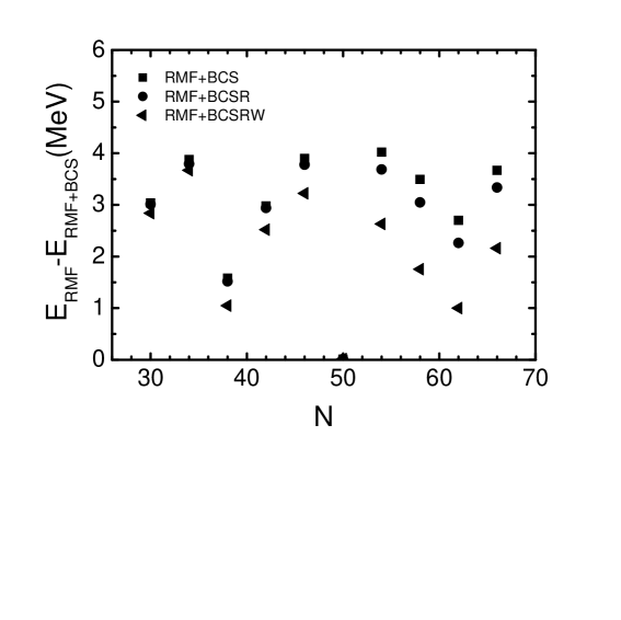
Figure 5: The pairing correlation energies $E_{BCS}$ calculated in Eq.(35) in the RMF+BCS, RMF+BCSR and RMF+BCSRW approaches. The notations are same as in Fig.1.

The $E_{BCS}$ of Ni isotopes calculated in various approaches are plotted in Fig.5. It is shown that the results produced in the three approaches are very close to each other for those isotopes not far away from the $\beta$ stable-line. It implies that the width of the resonance in the pairing correlation could be neglected at $N\leq 34$. The RMF+BCS and RMF+BCSR give more or less similar values of $E_{BCS}$, even near the drip line. The width effect gets more and more pronounced as the neutron number increases, especially near the drip line. Therefore a proper treatment of the resonant continuum including its width might be necessary for the nuclei near the drip line.

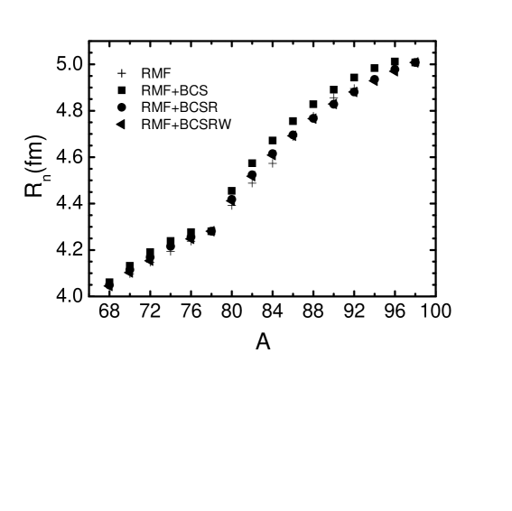
Figure 6: Neutron rms radii for neutron rich even-even Ni isotopes calculated in the RMF, RMF+BCS, RMF+BCSR, and RMF+BCSRW approaches with parameter set NL3. The notations are same as in Fig.4

Neutron rms radii of neutron rich even-even Ni isotopes are further calculated in the three approaches, which are plotted in Fig.6. The rms radii calculated in the RMF are also shown in Fig.6 and displayed by cross. It is seen that neutron rms radii of Ni isotopes at $A<80$ calculated in all approaches are very close to each other, which is similar to what was observed in the binding energy. The neutron rms radii calculated in the RMF+BCS with a box become larger at $A>80$ in comparison with those produced in other approaches. This is due to the fact that the contribution of the pairing correlation from the scattering states $3p_{3/2}$ and $3p_{1/2}$ is included in the RMF+BCS calculations. They are not resonant states and their wave functions are not well localized inside the nucleus. The neutron rms radius for ⁸⁴Ni given in the RMF is slightly smaller than that obtained in the other approaches. Actually this is a natural result when the pairing correlation is switched on. The neutron rms radius in the RMF+BCS is increased because the pairing interaction scatters some neutrons from $2d_{5/2}$ to the loosely bound state $3s_{1/2}$ which is a state less localized. In contrast, in the case of ⁹⁰Ni the states $3s_{1/2}$ and $2d_{3/2}$, which are completely occupied in the RMF approximation are scattered to states $1g_{7/2}$ and $1h_{11/2}$ due to the pairing interaction. Although the states $1g_{7/2}$ and $1h_{11/2}$ are close to or buried in the continuum, their wave functions are more localized inside the nucleus than those for the $3s_{1/2}$ and $2d_{3/2}$ states due to a high centrifugal barrier. Therefore the rms radius of ⁹⁰Ni calculated in the RMF is larger than that produced in calculations including the pairing correlation.

We plot the neutron density of ⁸⁴Ni in Fig.7, where the dash-dotted curve is obtained in the RMF, the short-dotted, dashed and solid curves are produced in the RMF+BCS, RMF+BCSR and RMF+BCSRW approaches, respectively. The tail of the density distribution gets larger when the pairing correlation is considered. The width effect on the density distribution is very small, which is consistent to the calculated neutron rms radii. In order to show the effect of the box size on the density in the box RMF+BCS approximation we also plot the neutron density with various values of the box size R${}_{\text{box}}$ = 15, 20, 25 fm in Fig.7. It is observed that the tail of the density strongly depends on the box size, where unphysical particle gas may appear in the exotic nucleus. In the RMF+BCS calculation non-resonant discretized states in the continuum are included in pairing correlation, such as $3p_{3/2}$ and $3p_{1/2}$ states. Their wave functions have a long tail strongly depending on the box size. It is found that this problem is well overcome when one performs the pairing correlation calculation with only a few narrow resonant states in stead of those discretized states in the continuum.

V Summary

In this paper, we have investigated the pairing correlation for neutron-rich Ni isotopes in the relativistic mean field theory and Bardeen-Cooper-Schrieffer approximation with a constant pairing strength. A proper treatment of the single particle resonant state in the continuum on pairing correlations has to include not only its energy, but also its width. The inclusion of the width of the resonant state in the pairings can be performed by introducing a level density in the continuum into the pairing gap equation. The resonant continuum is solved by imposing a proper scattering boundary condition. The investigation is performed in three approaches: RMF+BCS, RMF+BCSR and RMF+BCSRW with the effective Lagrangian parameter set NL3. A special attention is paid on the width effect of resonant states in the continuum on the pairing correlation for nuclei close to the drip line. We have studied the width effect of the resonant continuum on pairings: pairing gap, Fermi energy and occupation probability, as well as nuclear ground state properties, such as binding energy, two-neutron separation energy, neutron rms radius and neutron density. The results show that a proper treatment of the resonant continuum in pairing correlations, which explicitly includes the width of the single particle resonant state is important for nuclei close to neutron drip line. They could affect the pairing gaps, Fermi energies, pairing energies, and binding energies considerably. Various RMF+BCS approaches could give a similar description on the ground state properties for nuclei not far away from the $\beta$ stable line. It is observed that unphysical particle gas, which may appear in the traditional mean field plus BCS calculation for nuclei in the vicinity of drip line can be well overcome when one performs pairing correlation calculations with only resonant states instead of discretized states in the continuum. It might be concluded that the simple BCS method works well in describing the pairing correlations for neutron rich nuclei provided the continuum is properly treated.

Table 1: The binding energies of Ni isotopes near the neutron drip line calculated in the RMF+BCS, RMF+BCSR, and RMF+BCSRW approaches with parameter set NL3. The available experimental binding energies of the Ni isotopes for $N\leq$50 from Ref.Audi95 are also shown. All energy values in the table are in unit of MeV.

	RMF+BCS	RMF+BCSR	RMF+BCSRW	Exp.
58Ni	502.347	502.275	502.104	506.453
60Ni	521.655	521.448	521.363	526.841
62Ni	540.458	540.374	540.251	545.258
64Ni	558.361	558.273	558.055	561.754
66Ni	575.642	575.579	575.009	576.830
68Ni	590.892	590.960	590.930	590.430
70Ni	603.233	603.195	602.775	602.600
72Ni	614.246	614.116	613.567	613.900
74Ni	624.428	624.307	623.752	623.900
76Ni	633.840	633.816	633.414	633.100
78Ni	642.352	642.555	642.555	641.400
80Ni	647.837	647.659	646.964
82Ni	652.279	651.943	650.888
84Ni	656.092	655.678	654.472
86Ni	659.422	658.975	657.682
88Ni	662.284	661.863	660.582
90Ni	664.756	664.319	663.047
92Ni	667.756	666.456	665.254
94Ni	668.562	668.319	667.144
96Ni	670.133	670.183	669.332
98Ni	671.382	671.605	671.605

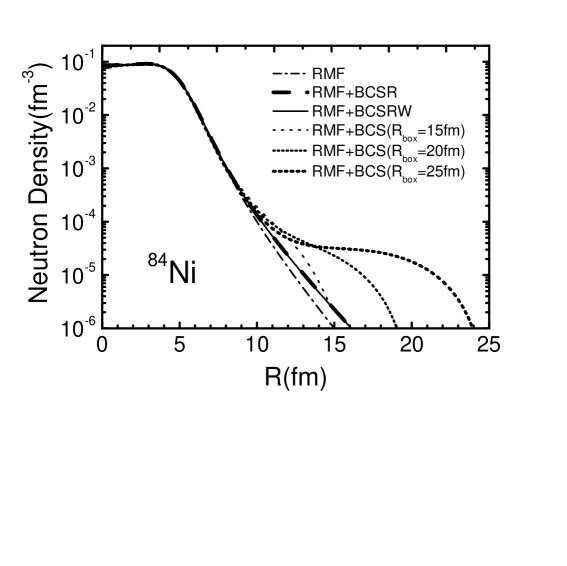
Figure 7: Neutron density distribution for ⁸⁴Ni calculated in the RMF, RMF+BCS, RMF+BCSR, and RMF+BCSRW approaches, where the RMF+BCS results calculated with various values of the box size R${}_{\text{box}}$ = 15, 20, 25 fm are also plotted.