Thermal analysis of production of resonances in relativistic heavy-ion collisions

Abstract

Production of resonances is considered in the framework of the single-freeze-out model of ultra-relativistic heavy ion collisions. The formalism involves the virial expansion, where the probability to form a resonance in a two-body channel is proportional to the derivative of the phase-shift with respect to the invariant mass. The thermal model incorporates longitudinal and transverse flow, as well as kinematic cuts of the STAR experiment at RHIC. We find that the shape of the $\pi^{+}\pi^{-}$ spectral line qualitatively reproduces the preliminary experimental data when the position of the $\rho$ peak is lowered. This confirms the need to include the medium effects in the description of the RHIC data. We also analyze the transverse-momentum spectra of $\rho$, $K^{*}(892)^{0}$, and $f_{0}(980)$, and find that the slopes agree with the observed values. Predictions are made for $\eta$, $\eta^{\prime}$, $\omega$, $\phi$, $\Lambda(1520)$, and $\Sigma(1385)$.

I Introduction

With the help of the mixed-event technique the STAR Collaboration has managed to obtain preliminary results on the production of hadronic resonances. The data were presented for $K^{*}(892)^{0}$ starKstar1 ; starKstar2 , $\rho(770)^{0}$ patricia1 ; patricia2 , $f_{0}(980)$ patricia1 ; patricia2 , and $\Lambda(1520)$ christelle ; markert ; ludovic . The invariant-mass distribution of the particles produced in the decays of the resonances may be used to get the information on the possible in-medium modifications of hadron masses. Such modifications are predicted by various theoretical models of dense and hot hadronic matter BR ; hatlee , as well as hinted by the enhancement of the dilepton production in the low-mass region CERES ; HELIOS . Most interestingly, the measured invariant-mass distribution of the $\pi^{+}\pi^{-}$ pairs patricia1 ; patricia2 also suggests a drop of the effective mass of the $\rho$ meson by several tens of MeV patricia1 . This effect was recently discussed by Shuryak and Brown shuryakbrown , Kolb and Prakash KolbP , and Rapp Rapp , with the conclusion drawn that it is a genuine dynamical effect induced by the interaction of the $\rho$ meson with the hadronic matter. On the other hand, the measurement of the invariant-mass distributions of the $\pi K$ pairs indicates that the effective mass of the $K^{*}(892)^{0}$ remains unchanged starKstar2 .

Since one measures the properties of stable hadrons which move freely to detectors, the experimentally obtained correlations may bring us information only about the final stages of the evolution of the hadronic matter, i.e., about the conditions at freeze-out. From this point of view it is interesting to analyze the production of resonances in the framework of the thermal approach (the single-freeze-out model of Refs. wbwf ; str ; zakop ) which turned out to be very successful in reproducing the yields and spectra of stable hadrons. In particular, the thermal model can be naturally used to study the impact of the possible in-medium modification of the $\rho$-meson mass on different physical observables, e.g., on the correlation in the invariant mass of the $\pi^{+}\pi^{-}$ pairs, the ratios of the resonance abundances, or their transverse-momentum spectra.

The paper is organized as follows: In the next Section we outline the Dashen-Ma-Bernstein formalism used to describe a gas of hadronic resonances. In Sec. III we present the invariant-mass correlations of $\pi^{+}\pi^{-}$ pairs emitted from a static thermal source, and in Sec. IV we discuss the effect of the temperature of such a source on the shape of the spectral $\pi^{+}\pi^{-}$ line. In Sec. V we present the main assumptions of the single-freeze-out model. With the knowledge of both the experimental kinematic cuts (Sec. VI) and the feeding from the decays of higher resonances (Sec. VII), the model is then used to compute the invariant mass spectrum of the $\pi^{+}\pi^{-}$ pairs (Sec. VIII). In Sec. IX and X we present the model results for the ratios of the resonance yields and for the resonance transverse-momentum spectra (wherever it is possible we compare the model results with the preliminary data). The paper contains three Appendices which give the parameters for the $\pi^{+}\pi^{-}$ phase shifts and explain in simple terms the implementation of the experimental kinematic cuts in our calculations of two- and three-body decays.

II Production of resonances and the phase-shifts

The formalism for the treatment of resonances in a hadronic gas in thermal equilibrium has been developed by Dashen, Ma, and Bernstein Da1 , and Dashen and Rajaraman Da2 , and in the context of heavy-ion physics has been recalled and further elaborated by Weinhold, Friman, and Nörenberg Wmsc ; WFNapp ; WFNnote ; WFNplb ; Wphd (see also denis ; larionov ; pelaez ). The basic formula following from the formalism is that density of the resonance per volume and per unit invariant mass, $M$, produced in the two-body channel of particles 1 and 2 in thermal equilibrium is given by the formula

$$\frac{dn}{dM}=f\int\frac{d^{3}p}{(2\pi)^{3}}\frac{1}{\pi}\frac{d\delta_{12}(M)}{dM}\frac{1}{\exp\left(\frac{\sqrt{M^{2}+{\bm{p}}^{2}}}{T}\right)\pm 1},$$ (1)

where $\delta_{12}(M)$ is the phase shift for the scattering of particles 1 and 2, $f$ is a spin-isospin factor, $T$ is the temperature, and the sign in the distribution function depends on the statistics. In practice, one may replace the distribution function by the Boltzmann factor, since the effects of the quantum statistics are numerically small.

As pointed out by the authors of Ref. WFNnote , in many works the spectral function of the resonance is used ad hoc as the weight in Eq. (1) instead of the derivative of the phase shift, which is the correct thing to do. For narrow resonances this does not make a difference, since then both the spectral function and the derivative of the phase shift peak very sharply at the resonance position, $m_{R}$, i.e., $d\delta_{12}(M)/dM\simeq\pi\delta(M-m_{R})$, and then one recovers the narrow-resonance limit

$$n^{\rm(narrow)}=f\int\frac{d^{3}p}{(2\pi)^{3}}\frac{1}{\exp\left(\frac{\sqrt{m_{R}^{2}+{\bm{p}}^{2}}}{T}\right)\pm 1}.$$ (2)

However, for wide resonances, or for effects of tails, the difference between the correct formula (1) and the one with the spectral function is very significant, not only conceptually but also numerically.

We first focus on the $\pi^{+}\pi^{-}$ scattering. We use the experimental phase shifts, which can be parameterized with simple formulas of Ref. pipipar :

$$\tan\left(\delta^{I}_{l}(M)\right)=\sqrt{1-m_{\pi}^{2}/M^{2}}\;q^{2l}$$ (3)

$$\times\frac{(A^{I}_{l}+B^{I}_{l}q^{2}+C^{I}_{l}q^{4}+D^{I}_{l}q^{6})(4m_{\pi}^{2}-s^{I}_{l})}{M^{2}-s^{I}_{l}},$$

where $q=\sqrt{M^{2}-4m_{\pi}^{2}}/2$, $m_{\pi}=139.57$ MeV is the mass of the charged pion, and the remaining parameters are listed in App. A. The relevant channels are $I=1$, $l=1$ ($\rho$), $I=0$, $l=0$ ($f_{0}$/$\sigma$), and $I=2$, $l=0$.

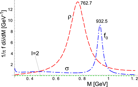
Figure 1: The weight functions, $1/\pi f\,d\delta/dM$, in the isoscalar, isovector, and isotensor channels, plotted as a function of the $\pi^{+}\pi^{-}$ invariant mass. The phase shifts are taken from the parameterization of the experimental data pipipar . Numerical labels indicate the peak positions (in MeV) which correspond to inflection points in the phase shifts as functions of $M$. The $I=2$ channel is negligible.

Figure 1 shows the weights in Eq. (1), i.e., the quantities $fd\delta(M)/(\pi dM)$, plotted as functions of $M$. The factor $f$ consists of the spin degeneracy, $2l+1$, and the isospin Clebsch-Gordan coefficient, equal $2/3$ for the isosinglet, $1$ for the isovector, and $1/2$ for the $I=2$ channel. In the isovector channel the peak of the weight function is found at $762.7$ MeV, which corresponds to the inflection point in $\delta(M)$, and not the point where $\delta(M)=\pi/2$, which is at $773.6$ MeV (note a 10 MeV “dropping” of the $\rho$-meson “mass”). For the isoscalar channel the corresponding curve in Fig. 1 peaks at 932.5 MeV. We note that in this channel the weight function $fd\delta/(\pi dM)$ is significantly different from the spectral function. The latter one appears in the calculation of the production rate (see for instance KolbP ; Rapp ), whereas our study concerns the invariant-mass spectra, where formula (1) holds. As a result of the use of the phase-shifts, there is a very small contribution from the $\sigma$ meson, since the strength of the scalar channel, as seen in Fig. 1, is small. It is worthwhile to notice that it peaks at the two-pion threshold pipipar , which is an immediate consequence of Eq. (3) for $l=0$. The contribution of the $I=2$ channel is tiny (also note that it is negative since the phase shift in this channel is a decreasing function of $M$, cf. Da2 ).

For three-body decays formulas analogous to Eq. (1) may be given, cf. Ref. Da1 ; Da2 . They would involve the detailed dynamical information on the decay process. For our purpose this is not necessary (the three-body decays feed the range of rather low invariant $\pi^{+}\pi^{-}$ masses) and also not practical, since the detailed information on the dynamical dependences of the appropriate transition matrices is not easy to extract from the experimental data. In our calculations we include the resonances decaying into three-body channels which are very narrow ($\omega$, $\eta$, and $\eta^{\prime}$). Thus, as is customary in similar applications, we only account for the phase-space dependence on the invariant mass $M$, and do not consider dynamical effects of the transition matrix.

III Resonances in the static source

First, in order to gain some experience, we consider the simplest case of the emission of particles from a static source. We will come back to a more realistic description incorporating the flow in Sec. V. We also assume in this Section the single-freeze-out hypothesis wbwf ; str ; zakop , hence no effects of rescattering are incorporated after the chemical freeze-out. We thus assume the chemical freeze-out temperature to be wfwbmm ; BM4 ; review

$$T_{\rm chem}=165~{}{\rm MeV},$$ (4)

and, as we have said, the thermal freeze-out occurs at the same temperature, $T_{\rm therm}=T_{\rm chem}$. In the next Section we will lift this assumption.

We now simply use Eq. (1) with $T=T_{\rm chem}$, and include the following resonances that couple to the $\pi^{+}\pi^{-}$ channel: $\rho$, $f_{0}$/$\sigma$, $\omega$, $\eta$, $\eta^{\prime}$, $K_{S}$, and $f_{2}(1270)$. For the omega, both the three-body mode, $\omega\to\pi^{+}\pi^{-}\pi^{0}$, and the two-body mode, $\omega\to\pi^{+}\pi^{-}$, are incorporated. The appropriate branching ratios are included in the constant $f$ in Eq. (1). For channels other than those of Fig. 1, where the experimental phase shifts are included, we use the simple Breit-Wigner parameterization, which is good for the narrow resonances. For the width of $K_{S}$ we take the experimental resolution of the STAR experiment, which is about $10$ MeV FachPriv . The width of the $\omega$ is also increased by the same value.

We compute the spectra at mid-rapidity, hence we use

$$\left.\frac{dn}{dMdy}\right|_{y=0} = \sum_{i}f_{i}\int_{p_{\perp}^{\rm low}}^{p_{\perp}^{\rm high}}\frac{p_{\perp}dp_{\perp}}{(2\pi)^{2}}\frac{1}{\pi}\frac{d\delta_{i}(M)}{dM}$$

$$\times\frac{\sqrt{M^{2}+p_{\perp}^{2}}}{\exp\left(\frac{\sqrt{M^{2}+{\bm{p}_{\perp}}^{2}}}{T}\right)-1},$$

where $i$ labels the channel, $n$ is the volume density of the $\pi^{+}\pi^{-}$ pairs, and $M$ is the invariant mass of the $\pi^{+}\pi^{-}$ system. The above formula, written for two-body decays, is supplemented in the actual calculation with the three-body reactions. The limits for the transverse-momentum integration are taken at the upper and lower cuts for the STAR experiment patricia2 , $p_{\perp}^{\rm low}=0.2~{}{\rm GeV}$ and $p_{\perp}^{\rm high}=2.2~{}{\rm GeV}$.

The results of the calculation are shown in Fig. 2(a). The two-body resonances lead to well-visible peaks, while the three-body channels of the $\omega$, $\eta$ and $\eta^{\prime}$ produce typical broad structures at lower values of $M$. Note that the scalar-isoscalar channel generates the resonance, $f_{0}$, and a smooth background, $\sigma$. This background increases with the decreasing $M$, and peaks at the threshold.

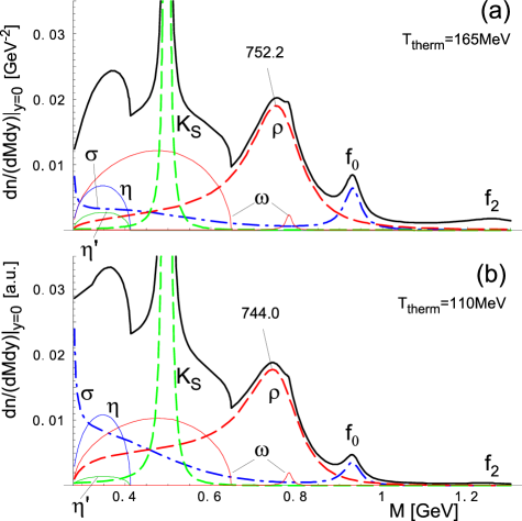
Figure 2: The volume density of the $\pi^{+}\pi^{-}$ pairs plotted as a function of the invariant mass, obtained from the thermal model with a static source, Eq. (III). (a) The case of $T_{\rm therm}=T_{\rm chem}=165~{}{\rm MeV}$. (b) The case of $T_{\rm therm}=110~{}{\rm MeV}$. The numbers indicate the position of the $\rho$ peak (in MeV). The labels indicate the decays included, with the two-body $\pi^{+}\pi^{-}$ channels and the three-body channels, $\omega\to\pi^{0}\pi^{+}\pi^{-}$, $\eta\to\pi^{0}\pi^{+}\pi^{-}$, and $\eta^{\prime}\to\eta\pi^{+}\pi^{-}$. The relative contributions from the resonances are fixed by the value of the temperature.

IV Chemical vs. kinetic freeze-out

In this section we analyze in simple terms the effects of possible lower temperature of the thermal freeze-out on the shape of the $\pi^{+}\pi^{-}$ invariant-mass correlations. To this end we simply use Eq. (III) at a lower value of $T$.

Consider, for brevity of notation, the gas consisting only of $\pi^{+}$, $\pi^{-}$, and $\rho^{0}$. We assume isospin symmetry for the system, which works very well for RHIC brahmsy . The pions rescatter elastically through the $\rho$-channel. The total number of pions that are observed in the detectors is equal to

$$N_{\pi} = V^{\rm chem}\left(2\times n_{\pi}(T_{\rm chem},\mu=0)\right.$$ (6)

$$+ \left.2\times 3\times n_{\rho}(T_{\rm chem},\mu=0)\right),$$

where

$$n_{i}(T,\mu)=\int\frac{d^{3}p}{(2\pi)^{3}}\exp\left(\frac{-\sqrt{m_{i}^{2}+{\bm{p}}^{2}}+\mu}{T}\right).$$ (7)

The factor of 2 in front of $n_{\pi}$ in Eq. (6) comes from the $\pi^{+}$-$\pi^{-}$ degeneracy, the factor of 2 in front of $n_{\rho}$ comes from the fact that rho decays into two pions, and the factor of 3 is the spin degeneracy of the $\rho$. The chemical potential, $\mu$, vanishes at the chemical freeze-out. The volume at the chemical freeze-out is denoted by $V^{\rm chem}$.

The chemical freeze-out is defined as the stage in the evolution when the abundances of stable (with respect to the strong interaction) particles have been fixed. Next, the system expands, and while it progresses in its evolution, the elastic scattering may occur. This scattering proceeds through the formation of unstable resonances, until the system is too dilute for the scattering to be effective and the thermal freeze-out occurs. At the moment of the thermal freeze-out the total number of pions in our example is

$$N_{\pi} = V^{\rm therm}\left(2\times n_{\pi}(T_{\rm therm},\mu_{\pi})\right.$$ (8)

$$+ \left.2\times 3\times n_{\rho}(T_{\rm therm},\mu_{\rho})\right),$$

where $V^{\rm therm}$ is the volume at the thermal freeze-out, $\mu_{\pi}$ and $\mu_{\rho}=2\mu_{\pi}$ (the reaction $\rho^{0}\leftrightarrow\pi^{+}\pi^{-}$ is in equilibrium) are the chemical potentials which ensure that $N_{\pi}$ is conserved, as requested by the fact that the system had frozen chemically. Knowing the ratio $V^{\rm therm}/V^{\rm chem}$ we could compute $\mu_{\pi}$ comparing the right-hand sides of Eqs. (6) and (8). However, for the present purpose, where we are only interested in the shape of the correlation function in $M$ and not the absolute values, this is not necessary. The chemical potential enters in Eq. (8) as a multiplicative constant, $V^{\rm therm}\exp(2\mu_{\pi}/T_{\rm therm})$. Since we do not control in the present calculation the volume, we can remove the normalization constant from our consideration. The argument holds if more reaction channels are present.

Thus, we redo the calculation of the previous Section, based on Eq. (III), but now with a lower temperature and an arbitrary normalization constant. The results for $T_{\rm therm}=110$ MeV are shown in Fig. 2 (b). We note a prominent difference from the case of Fig. 2 (a), where the temperature was significantly higher: the high-$M$ spectrum is suppressed, while the low-$M$ spectrum is enhanced. Beginning from the high-mass end, we notice that the $f_{2}$ resonance has practically disappeared, the relative strength of the $f_{0}$ to the $\rho$ peak is only about 1/5 compared to 1/3 in Fig. 2 (a), finally, left to the $K_{s}$ peak we note a significantly larger background from the $\sigma$ tail, the shoulder of the $\rho$, and the $\eta$ decays. While for $T=165$ MeV the hight of this background is only slightly above the hight of the $\rho$ peak, for $T=110$ MeV it rises to about two times the hight of the $\rho$ peak.

We also remark that due to the presence of the thermal function in Eq. (III), the position of the peak is shifted downwards from the original vacuum value to 752.2 MeV for $T_{\rm therm}=165$ MeV, and to 744.0 MeV for $T_{\rm therm}=110$ MeV.

To conclude this Section, we state that the very simple thermal analysis shows that the shape of the “spectral line” of the $\pi^{+}\pi^{-}$ system depends strongly on the temperature of the thermal freeze-out, which, when compared to accurate data, may be used to determine $T_{\rm therm}$ in an independent manner. In the next sections we elaborate on this observation by incorporating other important effects.

V Flow and the single-freeze-out model

The medium produced at mid-rapidity in ultra-relativistic heavy-ion collisions undergoes a rapid expansion, characterized by the longitudinal and transverse flow. Although flow has no effect on the invariant mass of a pair of particles produced in a resonance decay, since the quantity is Lorentz-invariant, it nevertheless affects the results, since the kinematic cuts imposed in the experiment in an obvious manner break this invariance. In Ref. wbwf ; str we have constructed a thermal model which includes the flow effects. The model has the following main ingredients:

1. There is one universal freeze-out, occurring at the temperature

   $$T_{\rm chem}=T_{\rm therm}\equiv T\simeq 165~{}{\rm MeV}.$$ (9)

   In wfwbmm ; wbwf ; str ; zakop we have demonstrated that with the inclusion of all hadronic resonances the distinction between the traditionally considered chemical and thermal freeze-outs is not necessary, at least for RHIC.

2. To describe the geometry and flow at the freeze-out we adopt the approach of Refs. bjorken ; baym ; Kolya ; siemens ; SSH ; BL ; cs1 ; Rischke ; SH ; cs2 . The freeze-out hypersurface is defined by the condition

   $$\tau=\sqrt{t^{2}-r^{2}_{x}-r^{2}_{y}-r^{2}_{z}}={\rm const},$$ (10)

   while the transverse size of the fire-cylinder is made finite by requesting that

   $$\rho\equiv\sqrt{r_{x}^{2}+r_{y}^{2}}<\rho_{\rm max}.$$ (11)

   In addition, we assume that the four-velocity of the expansion at freeze-out is proportional to the coordinate, namely

   $$u^{\mu}=\frac{x^{\mu}}{\tau}=\frac{t}{\tau}\left(1,\frac{r_{x}}{t},\frac{r_{y}}{t},\frac{r_{z}}{t}\right).$$ (12)

   The model is explicitly boost-invariant, which in view of the recent data delivered by BRAHMS brahmsy is justified for the description of particle production in the rapidity range $-1<y<1$.

3. All resonances from the Particle Data Tables PDG are included in the calculation, which is important due to the Hagedorn-like behavior of the resonance mass spectrum hagedorn ; myhag ; bled ; rafhag .

The model has altogether four parameters: two thermal parameters, $T$, and the baryon chemical potential, $\mu_{B}$, which are fitted to the available particle ratios, and two geometric parameters, $\tau$ and $\rho_{\rm max}$, fitted to the transverse-momentum spectra. The details of the model can be found in Ref. zakop . The model works very well and economically for the particle ratios wfwbmm , transverse-momentum spectra wbwf , as well as strange-particle production str .

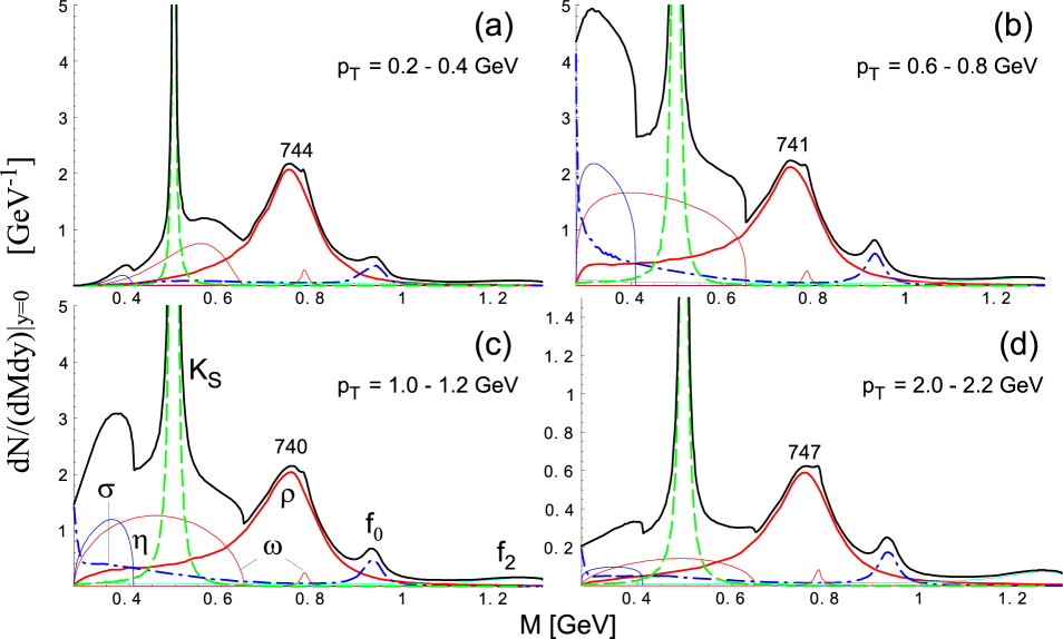
Figure 3: The invariant $\pi^{+}\pi^{-}$ mass spectra in the single-freeze-out model for four sample bins in the transverse momentum of the pair, $p_{T}$, plotted as a function of $M$. The contribution of various resonances are labeled in Fig. (c), with $\eta$ indicating the joint contribution of $\eta$ and $\eta^{\prime}$. The kinematic cuts of the STAR experiment are incorporated. The labels at the $\rho$ peak indicate its position in MeV, lowered as compared to the vacuum value due to thermal effects.

VI Kinematic cuts

The next important effect is related to the experimental cuts and traditionally has been the domain of experimentalists. However, in the present application the inclusion of all relevant kinematic cuts of the STAR analysis patricia1 ; patricia2 ; FachPriv can be included straightforwardly. Needless to say that the proper inclusion of kinematic constraints is frequently crucial when comparing theoretical models to the data.

For two-body decays, the relevant formula for the number of pairs of particles $1$ and $2$, derived in App. B, has the form

$$\frac{dN_{12}}{dM} = \frac{d\delta_{12}}{dM}{\frac{bm}{p_{1}^{\ast}}}\int_{p_{1,\rm{low}}^{\perp}}^{p_{1,{\rm high}}^{\perp}}\!\!\!\!\!dp_{1}^{\perp}\int_{y_{1,{\rm low}}}^{y_{1,{\rm high}}}\!\!\!\!\!dy_{1}\int_{p_{\rm low}^{\perp}}^{p_{\rm high}^{\perp}}\!\!\!\!\!dp^{\perp}\int_{y_{\rm low}}^{y_{\rm high}}\!\!\!\!\!dy$$ (13)

$$\times C_{2}^{0}C^{\eta}_{1}C^{\eta}_{2}\,\frac{\theta(1-\cos^{2}\gamma_{0})}{|\sin\gamma_{0}|}S(p^{\perp}),$$

with all quantities defined in App. B.

For the case of three-body decays we have

$$\frac{dN_{12}}{dM} = b\int_{0}^{\infty}2\pi p^{\perp}dp^{\perp}\int_{-\infty}^{\infty}dy\frac{dN_{12}({\bm{p}}^{\perp},y)}{dM}S(p^{\perp}),$$

(14)

where $b$ is the branching ratio and $dN_{12}({\bm{p}}^{\perp},y)/dM$ has been evaluated in App. C, with full inclusion of all cuts relevant in the STAR experiment.

The cuts in the STAR analysis of the $\pi^{+}\pi^{-}$ invariant-mass spectra have the following form patricia1 ; patricia2 ; FachPriv :

$$|y_{\pi}| \leq 1,$$

$$|\eta_{\pi}| \leq 0.8,$$ (15)

$$p^{\perp}_{\pi} \geq 0.2~{}{\rm GeV},$$

while the bins in $p_{T}\equiv|{\bm{p}}_{\pi}^{\perp}+{\bm{p}}_{\pi}^{\perp}|$ start from the range $0.2-0.4$ GeV, and step up by $0.2$ GeV until the range $2.2-2.4$ GeV. These conditions are implemented in the calculation shown below.

VII Decays of higher resonances

An important ingredient and, in fact, the key to the success of the thermal models in both reproducing the particle ratios and the transverse-momentum spectra wfwbmm ; wbwf ; str ; zakop , is the inclusion of resonances. Although the thermal distribution suppresses the high-mass particles, their abundance grows exponentially according to the Hagedorn hypothesis hagedorn ; myhag ; bled ; rafhag , and in practice one needs to go very high up in the mass of the resonances in order to obtain stable results mm . We include all resonances from the Particle Data Tables PDG . The high-lying resonances decay in cascades, eventually producing stable particles.

The resonances considered in this paper, in particular the $\rho$, also acquire substantial contributions from the higher resonances, e.g., $\eta^{\prime}\to\rho^{0}\gamma$, or $\phi(1020)\to\rho\pi$. Such effects, entering at the level of a few tens of %, are difficult to account for accurately in our formalism. This is due to the dynamics characterized by the parameters that are not well known. For instance, the decay of $\eta^{\prime}$ may proceed through the $\rho^{0}\gamma$ channel, as well as directly into the uncorrelated three-pion state, $\pi^{+}\pi^{-}\pi^{0}$, which forms a smooth background around the $\rho$ peak. In other words, the feeding of the $\rho$ from the higher resonance need not reproduce the shape of the $\rho$ peak from Fig. 1, and the resulting dependence on $M$ may be altered to some extent. This important but, due to experimental uncertainties, not easy issue is left for later studies. At the moment we take the simplest way, and assume that the shape of the spectral line in Fig. 1 is not altered. This amounts to including a multiplicative factor, $d$, for each considered resonance. These factors are obtained from the thermal model as discussed in Ref. wfwbmm ; zakop . The thermal parameters for the full RHIC energy of $\sqrt{s_{NN}}=200$ GeV are abwbwf

$$T = 165.6{\rm~{}MeV},$$

$$\mu_{B} = 28.5{\rm~{}MeV},$$

$$\mu_{S} = 6.9{\rm~{}MeV},$$

$$\mu_{I} = -0.9{\rm~{}MeV}.$$ (16)

The calculation leads to the following enhancement factors coming from the decays of higher resonances: $d_{K_{S}}=1.98$, $d_{\eta}=1.74$, $d_{\sigma}=1.13$, $d_{\rho}=1.42$, $d_{\omega}=1.43$, $d_{\eta^{\prime}}=1.08$, $d_{f_{0}}=1.01$, and $d_{f_{2}}=1.28$. Thus, the effects is strongest for light particles, $K_{S}$, $\eta$, $\rho$, and $\omega$, while it is weaker for the heavier $\eta^{\prime}$ and scalar mesons.

VIII Results of the single-freeze-out model

We may finally come to presenting the results of the calculation in the framework of the single-freeze-out model. The calculation includes the kinematic cuts described in App. B and C, and the enhancement factors from the higher resonances, $d_{i}$, described in Sec. VII. The expansion parameters are taken to be $\tau=5$ fm and $\rho_{\rm max}=4.2$ fm, which according to the fits of the $p_{\perp}$ spectra, corresponds to the centrality 40-80% abwbwf . In Fig. 3 we show the results obtained with the help of Eqs. (13,14) with the STAR kinematic cuts (15), for four sample bins in the transverse momentum of the pair, $p_{T}$, with the lowest $p_{T}$ in Fig. 3(a) and highest in Fig. 3(d). The contributions of various resonances are clearly visible. We note that the shape of the spectrum changes with the assumed $p_{T}$ bin. For both the lowest and the highest $p_{T}$ the low-$M$ region is suppressed, while at intermediate $p_{T}$ the spectrum has large contributions at low $M$. In our calculation the relative contributions form various resonances is fixed, as given by the model. Also, the relative normalization between Figs. (a-d) is preserved. The labels at the $\rho$ peak indicate its position in MeV. We observe that it is lowered compared to the vacuum value, due to the thermal effects, and assumes values between 740 and 747 MeV. This fall is not as large as that observed in the preliminary STAR data patricia1 ; patricia2 , where the position of the peak resulting from fitting the data is much lower, about 700 MeV. Our single-freeze-out model with the vacuum $\rho$ meson is not capable of producing this result.

This is perhaps the most important outcome of our analysis: both the naive thermal approach, cf. Fig. 2, and the full-fledged single-freeze-out model with expansion and kinematic cuts, are unable to reproduce the (preliminary) STAR data if the vacuum value of the $I=1$ $\pi\pi$ phase shift (3) is used. This confirms the earlier conclusions of Shuryak and Brown shuryakbrown and Rapp Rapp . The model with the vacuum $\rho$ can bring the peak down to $\sim 740$ MeV, calling for about additional 40 MeV from other effects, such as the medium modifications.

Figure 4: Same as Fig. 3(c) with the $\rho$ meson scaled down by 9%. Now the peak of the $\rho$ has moved to the preliminary value observed in the STAR experiment patricia1 ; patricia2 .

In order to show how the medium modifications will show up in the $\pi^{+}\pi^{-}$ spectrum, we have scaled the $\pi\pi$ phase shift in the $\rho$ channel, according to the simple law

$$\delta^{1}_{1}(M)_{\rm scaled}=\delta^{1}_{1}(s^{-1}M)_{\rm vacuum},$$ (17)

where $s$ is the scale factor. We use $s=0.91$, which places the peak at 700 MeV. The result of this calculation is shown in Fig. 4. Now, with the lowered $\rho$ position, the calculation looks very similar to the preliminary data of Ref. patricia1 ; patricia2 . With the $\rho$ peak moved to the left the dip between the $\rho$ and $K_{S}$ peaks is largely reduced, as seen in the preliminary data. Also, the background on the left side of the $K_{S}$ peak, coming from other resonances, is, for the considered $p_{T}$ bin, significantly higher than the hight of the $\rho$ peak.

We also remark that the shape of the the curves obtained in the single-freeze-out model for intermediate values of $p_{T}$ is closer to the naive thermal-model calculation of Fig. 2 with $T_{\rm therm}=110$ MeV rather than $T_{\rm therm}=165$ MeV. This is reminiscent of the “cooling” effect of the resonance decays, cf. Ref. wfwbmm . Indeed, the enhancement factors $d_{i}$, higher for low mass $M$ and lower for high mass $M$, connected with the feeding of the resonances by even higher excited states, lead to the modification of the spectral line such that it resembles a lower temperature spectrum obtained without the resonance feeding.

	Model $m^{*}_{\rho}=770$ MeV	Model $m^{*}_{\rho}=700$ MeV	Experiment
$T$ [MeV]	$T=165.6\pm 4.5$	$T=167.6\pm 4.6$
$\mu_{B}$ [MeV]	$\mu_{B}=28.5\pm 3.7$	$\mu_{B}=28.9\pm 3.8$
$\eta/\pi^{-}$	$0.120\pm 0.001$	$0.112\pm 0.001$
$\rho^{0}/\pi^{-}$	$0.114\pm 0.002$	$0.135\pm 0.001$	$0.183\pm 0.028$ patricia2 (40-80%)
$\omega/\pi^{-}$	$0.108\pm 0.002$	$0.102\pm 0.002$
$K^{*}(892)/\pi^{-}$	$0.057\pm 0.002$	$0.054\pm 0.002$
$\phi/\pi^{-}$	$0.025\pm 0.001$	$0.024\pm 0.001$
$\eta^{\prime}/\pi^{-}$	$0.0121\pm 0.0004$	$0.0115\pm 0.0003$
$f_{0}(980)/\pi^{-}$	$0.0102\pm 0.0003$	$0.0097\pm 0.0003$	$0.042\pm 0.021$ patricia2 (40-80%)
$K^{*}(892)/K^{-}$	$0.33\pm 0.01$	$0.33\pm 0.01$	$0.205\pm 0.033$ patricia2 (0-10%) $0.219\pm 0.040$ patricia2 (10-30%) $0.255\pm 0.046$ patricia2 (30-50%) $0.269\pm 0.047$ patricia2 (50-80%)
$\phi/K^{*}(892)$	$0.446\pm 0.003$	$0.448\pm 0.002$	$0.595\pm 0.123$ patricia2 (0-10%) $0.633\pm 0.138$ patricia2 (10-30%) $0.584\pm 0.132$ patricia2 (30-50%) $0.528\pm 0.106$ patricia2 (50-80%)
$\Lambda(1520)/\Lambda$	$0.061\pm 0.002$	$0.062\pm 0.002$	$0.022\pm 0.010$ ludovic (0-7%) $0.025\pm 0.021$ ludovic (40-60%) $0.062\pm 0.027$ ludovic (60-80%)
$\Sigma(1385)/\Sigma$	$0.484\pm 0.004$	$0.485\pm 0.004$

Table 1: Predictions of the thermal model for the ratios of hadronic resonances measured at RHIC at $\sqrt{s_{NN}}=200$ GeV. In the two model calculations, the two different effective masses of the $\rho$ meson have been assumed. In the first case (second column) $m^{*}_{\rho}=770$ MeV, whereas in the second case (third column) $m^{*}_{\rho}=700$ MeV. The two thermodynamic parameters have been fitted only to the ratios of stable hadrons. In the first case they are the same as those discussed in Sec. 2. The preliminary experimental data are taken from patricia2 ; ludovic . Both the experimental and the theoretical pion yields are corrected for the weak decays.

IX Ratios of the resonance yields

In this and the next Section we present the results of the single-freeze-out model for the ratios of the resonance yields and the resonance transverse-momentum spectra. In our analysis we shall consider two cases: in the first (standard) case we assume that the masses of hadrons are not changed by the in-medium effects, whereas in the second case we assume that the mass of the $\rho$ meson at freeze-out is smaller than its vacuum mass. Inspired by the preliminary STAR results patricia1 ; patricia2 , we shall use for this purpose a rather low value of $m^{*}_{\rho}=700$ MeV. In these two cases the values of the thermodynamic parameters are determined from the experimental ratios of the yields of stable hadrons (those listed in Table 1 of Ref. abwbwf ). This gives $T=165.6\pm 4.5$ MeV and $\mu_{B}=28.5\pm 3.7$ MeV for the standard case abwbwf , and $T=167.6\pm 4.6$ MeV and $\mu_{B}=28.9\pm 3.8$ MeV for the case with the modified mass of the $\rho$ meson. The reason for not including the ratios of the resonance yields as the input in our appraoch is twofold: firstly, the data describing the production of the resonances are preliminary; secondly, there are no measurements of the resonance spectra in the central events. For example, the data on $\rho^{0}$ production were collected for the centrality class 40-80%.

We take into consideration the modification of the mass of the $\rho$ meson only, since at the moment there are no experimental hints concerning the behaviour of the masses of other resonances (except for the mass of $K^{*}(892)^{0}$ which is not changed). In Ref. mmwfwb-inmedium we studied the effect of the in-medium mass and width modifications on the outcome of the thermal analysis in the situation where a common scaling of baryon and meson masses with the temperature or the density was assumed (only the masses of the pseudo-Goldstone bosons were kept constant). The results of Ref. mmwfwb-inmedium showed that moderate modification particle masses are admissible. A satisfactory description of the ratios of hadron abundances measured at CERN SPS may be obtained in a thermal approach with the modified masses of hadronic resonances, however, the changes of the masses affect the values of the optimum thermodynamic parameters. Similar results were obtained from the analysis of the first RHIC data mm . The effects of the in-medium mass and width modifications on the outcome of the thermal analysis were also studied in Refs. wfwb-inmedium ; hirschegg-inmedium ; zschiesche1 ; zschiesche2 ; renk .

Our predicitions for the ratios of the resonance yields are presented in Table 1. The most interesting are the results for the $\rho^{0}/\pi^{-}$ ratio which is 0.11 for the case without the in-medium modifications and 0.14 for the case with the modified rho mass. The first value is in a good agreement with a theoretical number presented recently by Rapp Rapp . We can see that the effect of the dropping $\rho$-meson mass helps us to get closer to the preliminary experimental result of 0.18, however the theoretical and the experimental values still differ by more than one standard deviation. Our model value for the ratio $f_{0}(982)/\pi^{-}$ is a factor of four smaller than central value of the preliminary experimental result. On the other hand, our results for $K^{*}(892)/K^{-}$ and $\Lambda(1520)/\Lambda$ are larger than the preliminary experimental values, whereas the $\phi/K^{*}(892)$ ratio agrees rather well with the experiment (cf. Table 1).

A comparison of the theoretical and experimental results for the ratios involving resonances is interesting from the point of view of the discussion on the decoupling temperature, $T_{\rm therm}$, i.e., the temperature characterizing the thermal freeze-out. If $T_{\rm therm}$ is significantly smaller than $T_{\rm chem}$ one expects rt1 ; rt2 ; heinzqgp that the measured ratios such as $K^{*}/K$ or $\rho^{0}/\pi^{-}$ are smaller than the values determined at the chemical freeze-out. This behavior is due to the readjustment of the resonance abundances (formed in elastic collisions) to the decreasing temperature on the path the system follows from $T_{\rm chem}$ down to $T_{\rm therm}$. Our results shown in Table 1 indicate that certain experimental ratios are indeed smaller (such as $K^{*}(892)/K^{-}$ or $\Lambda(1520)/\Lambda$ for central collisions), whereas some are larger ($\rho^{0}/\pi^{-}$ and $f_{0}(982)/\pi^{-}$). Consequently, from the comparison of the theoretical and experimental ratios, at the moment, it is hard to draw a definite conclusion about the difference between the two freeze-outs. The study gets even more involved in view of possible in-medium modifications of the masses, which affect the ratios and may complicate the overall thermodynamic picture.

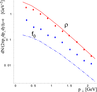
Figure 5: The mid-rapidity transverse-momentum spectra of the $\rho^{0}$ and $f_{0}(980)$ mesons, as obtained from the single-freeze-out model. The model parameters, $\tau=5$ fm and $\rho_{\rm max}=4.2$ fm, correspond to centralities $40-80$ % abwbwf . The data points are taken from Ref. patricia2 . The vacuum value of the $\pi\pi$ phase shift is used in the model calculation, with the scaled phase shift yielding very similar results.

X Transverse-momentum spectra

In this Section we present the single-freeze-out model results for the transverse-momentum spectra of various hadronic resonances. The method of the calculation is the same as that used in the calculation of the spectra of stable hadrons wbwf ; str ; zakop . In particular, the feeding of the resonance states from all known higher excited states is included, which leads to the enhancement of the resonance production characterized by the factors $d_{i}$. As usual, the two thermodynamic parameters and the two geometric parameters (fitted separately for different centrality windows) are taken from Ref. abwbwf . Knowing the centrality dependence of $\tau$ and $\rho_{\rm max}$ we may analyze the resonance production at different centralities and compare it to the existing data (note that the data on $\rho$ production are collected only for rather peripheral collisions corresponding to the centrality window 40-80%).

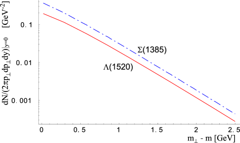
Figure 6: The single-freeze-out model predictions for the mid-rapidity transverse-mass spectra of $\Lambda(1520)$ and $\Sigma(1385)$. The model parameters, $\tau=8.7$ fm and $\rho_{\rm max}=7.2$ fm, correspond to the most central events, $c=0-20$% abwbwf .

In Fig. 5 we show our results for the transverse-momentum spectra of $\rho^{0}$ and $f_{0}(892)$, and compare them to the preliminary data obtained by the STAR Collaboration patricia2 . The expansion parameters are $\tau=5$ fm and $\rho_{\rm max}=4.2$ fm, which corresponds to the centrality of 40-80% abwbwf . In the presented calculation the vacuum value of the $\pi\pi$ phase shift has been used. We have checked that the scaled phase shift gives very similar results, and the small change of the thermodynamic parameters due to the drop of the rho mass affects the spectrum very little. The results shown in Fig. 5 indicate that our model can quite well reproduce the experimental spectrum of the rho meson and the slope of the $f_{0}(980)$ spectrum. We find, however, the discrepancy in the normalization between the model and the preliminary experimental data for the $f_{0}(980)$ spectrum, which reflects the result of Table 1. In Fig.  6 we show our predictions for the spectra of $\Lambda(1520)$ and $\Sigma(1350)$. Since $\Lambda(1520)$ is currently measured in the central collisions ludovic , in this case we used the values of the geometric parameters corresponding to the most central collisions, namely $\tau=8.7$ fm and $\rho_{\rm max}=7.2$ fm, which corresponds to centrality of $0-20$% abwbwf . In Fig. 6 we also show the spectrum of $\Sigma(1385)$ which might be measured by STAR in the near future christelle . In Fig. 7 we compare our predictions for the spectrum of $K^{\ast}(892)$ to the preliminary experimental results starKstar1 . To complete our discussion, we also show our predictions for other resonances for the most-central case, namely $\eta$, $\rho$, $\omega$, $\phi$, and $\eta^{\prime}$ and $f_{0}$.

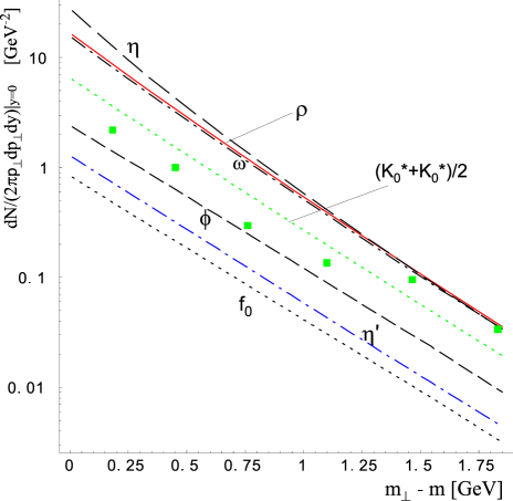
Figure 7: The mid-rapidity transverse-momentum spectra of the various resonances, as obtained from the single-freeze-out model. The preliminary data for the $K^{\ast}$ are taken from Ref. starKstar1 . The model parameters, $\tau=8.7$ fm and $\rho_{\rm max}=7.2$ fm, correspond to centralities $0-20$ % abwbwf .

XI Conclusion

In this paper we have presented a comprehensive analysis of resonance production at RHIC in the thermal approach. We have studied the $\pi^{+}\pi^{-}$ invariant mass spectra, the ratios of the resonances, and their transverse-momentum spectra.

Our calculation of the invariant mass distribution of the $\pi^{+}\pi^{-}$ pairs, performed in the framework of the single-freeze-out model, has been done with the use of the derivatives of the experimental phase shifts (and not the spectral function), which guarantees the thermodynamic consistency of our approach. Decays of higher resonances have been included in a complete fashion. Moreover, we have taken carefully into account the realistic kinematic cuts corresponding to the STAR experimental acceptance. We find that the preliminary STAR result indicating a drop of the rho meson mass down to 700 MeV cannot be reproduced in our model when the vacuum properties of the $\rho$ are used. A good qualitative agreement is found, however, when the mass of the $\rho$ is lowered. Therefore our calculation confirms the dropping-mass scenario for the $\rho$, induced by the medium effects.

We stress that the shape of the $\pi^{+}\pi^{-}$ spectrum is very sensitive to the freeze-out temperature. In a sense, it can be used as a “termometer”, independent of other methods of determining the temperature, such as the study of the ratios of the stable particles, or the slopes of the transverse momenta. We have shown that at small $T$ the contributions from the low lying resonances are enhanced, and the contributions at high mass are suppressed. On the contrary, at large $T$ the contributions from the high lying states are enhanced and become visible (like, e.g., the contribution from $f_{2}(1270)$), while the low mass contributions are reduced. In the single-freeze-out model, although the freeze-out process takes place at relatively high temperature $T\sim$ 165 MeV, the decays of the resonances lead to an effective “cooling” of the spectrum, with low-mass resonances acquiring more feeding from the higher states than the high-mass resonances. This would be equivalent to taking a lower temperature in a naive calculation without the resonance decays. Such effects, seen initially in the shape of the transverse-momentum spectra, are therefore also seen in the invariant mass $\pi^{+}\pi^{-}$ distributions.

The experimental information on the resonance production is crucial for our understanding of the freeze-out process. In particular, it may be used to distinguish between the scenario with the two freeze-outs, separate for the elastic and inelastic processes, and the scenario with a single freeze-out. For example, in the scenario with the two distinct freeze-outs the ratios involving the resonace yield in the numerator and the stable-hadron yield in the denominator (e.g., $\rho/\pi$, $K^{*}/K$, or $\Lambda(1520)/\Lambda$) should be smaller than the analogous ratio calculated at the chemical freeze-out. By comparing the preliminary STAR data to the predictions of the thermal model we have pointed out that certain ratios of this type are indeed somewhat smaller, while other are larger. Consequently, at the present time one cannot exclude which approximation, the one with two or the one with one freeze-out, is more appropriate in the thermal approach. More acurate data would be highly desired in that regard.

Appendix A Parameters for the $\pi\pi$ phase shifts

The following parameterization is used for the $\pi\pi$ phase shifts of Eq. (3) pipipar (all in units of $m_{\pi^{+}}=139.57$ MeV):

$$A_{0}^{0} = 0.220,\;A^{1}_{1}=0.379\cdot 10^{-1},\;A^{2}_{0}=-0.444\cdot 10^{-1},$$

$$B_{0}^{0} = 0.268,\;B^{1}_{1}=0.140\cdot 10^{-4},\;B^{2}_{0}=-0.857\cdot 10^{-1},$$

$$C_{0}^{0} = -0.0139,\;C^{1}_{1}=-0.673\cdot 10^{-4},\;C^{2}_{0}=-0.00221,$$

$$D_{0}^{0} = -0.00139,D^{1}_{1}=0.163\cdot 10^{-7},D^{2}_{0}=-0.129\cdot 10^{-3},$$

$$s_{0}^{0} = 36.77,\;s^{1}_{1}=30.72,\;s^{2}_{0}=-21.62.$$ (18)

Appendix B Kinematic cuts for two-body decays

Let the unlabeled quantities refer to the decaying resonance, and labels $1$ and $2$ to the decay products. The number of pairs coming from the decays of the resonance formed on the freeze-out hypersurface is ornik ; zakop

$${N}_{12}=\int\frac{d^{3}p_{1}}{E_{1}}C_{1}\int\frac{d^{3}p}{E}CC_{2}B\left(p,p_{1}\right)S(p),$$ (19)

where the symbols $C$, $C_{1}$, and $C_{2}$ denote kinematic cuts, and the source function of the decaying resonance is obtained from the Cooper-Frye formula CF1 ; CF2 ,

$$S(p)=\int d\Sigma_{\mu}\left(x\right)\,p^{\mu}\,\,f\left[p\cdot u\left(x\right)\right].$$ (20)

The quantity $f$ is the thermal distribution of the particle decaying at the hypersurface $\Sigma$, with the collective flow described by the four-velocity $u$. We pass to rapidity and transverse momentum variables in the laboratory frame, and have explicitly

$$B(p,p_{1})={\frac{b}{4\pi p_{1}^{\ast}}}\delta\left({\frac{p\cdot p_{1}}{m}}-E_{1}^{\ast}\right)$$ (21)

$$={\frac{b}{4\pi p_{1}^{\ast}}}\delta\left({\frac{m^{\perp}m_{1}^{\perp}\cosh(y-y_{1})-p^{\perp}p_{1}^{\perp}\cos\gamma}{m}}-E_{1}^{\ast}\right),$$

where $p_{1}^{\ast}$ and $E_{1}^{\ast}$ denote the momentum and energy of particle $1$ in the rest frame of the decaying resonance, $\gamma$ is the angle between ${\bm{p}}^{\perp}$ and ${\bm{p}}_{1}^{\perp}$ in the laboratory frame, and $b$ is the branching ratio for the considered decay channel.

In general, for the considered cylindrical symmetry, we have

$$C = \theta(p_{\rm low}^{\perp}\leq p^{\perp}\leq p_{\rm high}^{\perp})\theta(y_{\rm low}\leq y\leq y_{\rm high}),$$ (22)

$$C_{i} = \theta(p_{i,{\rm low}}^{\perp}\leq p_{i}^{\perp}\leq p_{i,{\rm high}}^{\perp})\theta(y_{i,{\rm low}}\leq y\leq y_{i,{\rm high}}),$$

with $i=1,2$ and $\theta(a\leq x\leq b)=1$ if the condition is satisfied, and $0$ otherwise. Due to momentum conservation we should use in (22)

$$p^{\perp}_{2} = \sqrt{\left(p^{\perp}\right)^{2}+\left(p_{1}^{\perp}\right)^{2}-2p^{\perp}p_{1}^{\perp}\cos\gamma}$$

$$y_{2} = \sinh^{-1}\left[\frac{m^{\perp}\sinh y-m_{1}^{\perp}\sinh y_{1}}{m_{\perp}}\right].$$ (23)

Next, we perform the integration over $\gamma$ in Eq. (19,21). The $\delta$ function gives the condition $\cos\gamma=\cos\gamma_{0}$, with

$$\cos\gamma_{0}=\frac{m^{\perp}m_{1}^{\perp}\cosh(y-y_{1})-mE_{1}^{\ast}}{p^{\perp}p_{1}^{\perp}},$$ (24)

which takes effect only if $-1\leq\cos\gamma_{0}\leq 1$. A factor of $2$ follows from the two solutions of $\gamma=\arccos(\cos\gamma_{0})$ for $\gamma\in[0,2\pi)$. The final result is

$${N}_{12} = {\frac{bm}{p_{1}^{\ast}}}\int_{p_{1,\rm{low}}^{\perp}}^{p_{1,{\rm high}}^{\perp}}\!\!dp_{1}^{\perp}\int_{y_{1,{\rm low}}}^{y_{1,{\rm high}}}\!\!dy_{1}\int_{p_{\rm low}^{\perp}}^{p_{\rm high}^{\perp}}\!\!dp^{\perp}\int_{y_{\rm low}}^{y_{\rm high}}\!\!dy$$ (25)

$$\times C_{2}^{0}\,\frac{\theta(-1\leq\cos\gamma_{0}\leq 1)}{\sin\gamma_{0}}S(p^{\perp}),$$

where we have introduced

$$C_{2}^{0}=\left.C_{2}\right|_{\cos\gamma=\cos\gamma_{0}},$$ (26)

with the substitution (23) understood.

The experimental cuts frequently involve cuts on pseudo-rapidity of particles. This amount to adding extra conditions of the form

$$\eta_{i}^{\rm low}\leq{1\over 2}\log\left(\frac{\sqrt{p_{i}^{\perp 2}+m_{i}^{\perp 2}{\rm sinh}^{2}y_{i}}+m_{i}^{\perp 2}{\rm sinh}^{2}y_{i}}{\sqrt{p_{i}^{\perp 2}+m_{i}^{\perp 2}{\rm sinh}^{2}y_{i}}-m_{i}^{\perp 2}{\rm sinh}^{2}y_{i}}\right)$$

$$\;\;\;\;\;\leq\eta_{i}^{\rm high},$$ (27)

which may be implemented in Eq. (25) in the form of $\theta$ functions, denoted by $C^{\eta}_{i}$.

The above formulas have been written for a sharp resonance. For a wide resonance, according to Eq. (1), the generalization assumes the form (13).

Appendix C Kinematic cuts for three-body decays

The three-body decay is usually considered in the rest frame of the resonance of mass $m$. Here, since the cuts are defined in the laboratory frame, we need to consider the kinematics in this frame. The phase-space integral for the decay of particle of mass $m$ and momentum ${\bm{p}}$ into products $1$, $2$, and $3$ is proportional to

$$\int\frac{d^{3}p_{1}}{E_{1}}\frac{d^{3}p_{2}}{E_{2}}\frac{d^{3}p_{3}}{E_{3}}C\delta\left(E-E_{1}-E_{2}-E_{3}\right)$$

$$\times\delta^{(3)}\left({\bm{p}}-{\bm{p}}_{1}-{\bm{p}}_{2}-{\bm{p}}_{3}\right)\left|\cal{M}\right|^{2},$$ (28)

where we have introduced $E=\sqrt{m^{2}+{\bm{p}}^{2}}$, etc, and $C$ denotes a generic cut in the kinematic variables, to be specified later. For simplicity we assume that $\cal{M}$ can be approximated by a constant, i.e. only the phase-space effect is included. This condition can be relaxed at no difficulty, if needed. We are interested in the invariant-mass distribution of particles $1$ and $2$, hence we introduce the $\delta[M-\sqrt{(E_{1}+E_{2})^{2}-({\bm{p}}_{1}+{\bm{p}}_{2})^{2}}]$ function in Eq. (28) and obtain the expression for the probability of emitting a pair of invariant mass $M$ from a particle moving with momentum ${\bm{p}}$:

$$\frac{dN_{12}({\bm{p}})}{dM} = a\int\frac{d^{3}p_{1}}{E_{{1}}}\frac{d^{3}p_{2}}{E_{{2}}}\frac{d^{3}p_{3}}{E_{{3}}}C\delta\left(E-E_{{1}}-E_{{2}}-E_{{3}}\right)$$ (29)

$$\times \delta\left(M-\sqrt{(E_{1}+E_{2})^{2}-({\bm{p}}_{1}+{\bm{p}}_{2})^{2}}\right)$$

$$\times \delta^{(3)}\left(\mathbf{p}-\mathbf{p}_{1}-\mathbf{p}_{2}-\mathbf{p}_{3}\right),$$

where $a$ is a normalization constant. First, we trivially carry the integration over ${\bm{p}}_{3}$ through the use of the last $\delta$ in Eq. (29). Next, we pass to the rapidity and transverse-momentum variables, and carry the integration over the angle between momenta ${\bm{p}}^{\perp}_{1}$ and ${\bm{p}}^{\perp}_{2}$, denoted as $\gamma$. This yields

$$\frac{dN_{12}({\bm{p}}^{\perp},y)}{dM} = 2\pi a\sum_{\epsilon}\int p_{1}^{\perp}dp_{1}^{\perp}dy_{1}d\alpha\int p_{2}^{\perp}dp_{2}^{\perp}dy_{2}C$$ (30)

$$\times \frac{1}{A}\frac{M}{p_{1}^{\perp}p_{2}^{\perp}|\sin\gamma_{0}|}\delta\left(A-E_{{3}}\right),$$

where $\alpha$ is the angle between ${\bm{p}}^{\perp}$ and ${\bm{p}}^{\perp}_{1}$,

$$\cos\gamma_{0}=\frac{-M^{2}+m_{1}^{2}+m_{2}^{2}+2m_{1}^{\perp}m_{2}^{\perp}{\rm cosh}(y_{1}-y_{2})}{2p_{1}^{\perp}p_{2}^{\perp}},$$

(31)

and the sum over $\epsilon$ results from the two solutions for $\gamma_{0}$, i.e. $\sin\gamma_{0}=\epsilon\sqrt{1+\cos^{2}\gamma_{0}}$. Next,

$$A=m^{\perp}{\rm cosh}y-m_{1}^{\perp}{\rm cosh}y_{1}-m_{2}^{\perp}{\rm cosh}y_{2},$$ (32)

and, finally,

$$E_{3} = \left[B-2p^{\perp}p^{\perp}_{1}\cos\alpha\right.$$

$$\left.-2p^{\perp}p^{\perp}_{2}\cos(\alpha-\gamma_{0})+2p_{1}^{\perp}p^{\perp}_{2}\cos\gamma_{0}\right]^{1/2},$$

with

$$B = m_{3}^{2}+(m^{\perp}{\rm sinh}y-m^{\perp}_{1}{\rm sinh}y_{1}-m^{\perp}_{2}{\rm sinh}y_{2})^{2}$$ (34)

$$+p^{\perp 2}+p_{1}^{\perp 2}+p_{1}^{\perp 2}.$$

We need still to carry the integration over the angle $\alpha$. We square the expression under the $\delta$ function in Eq. (30), obtaining

$$A^{2}=B-2p^{\perp}p^{\perp}_{1}\cos\alpha$$ (35)

$$-2p^{\perp}p^{\perp}_{2}(\cos\alpha\cos\gamma_{0}-\sin\alpha\sin\gamma_{0})+2p_{1}^{\perp}p^{\perp}_{2}\cos\gamma_{0}.$$

The squaring imposes the condition

$$A\geq 0.$$ (36)

This equation can be solved straightforwardly by introducing $t=\tan(\alpha/2)$,

$$\cos\alpha = \frac{1-t^{2}}{1+t^{2}},$$

$$\sin\alpha = \frac{2t}{1+t^{2}},$$ (37)

and the notation

$$G = \frac{-A^{2}+B+2\cos\gamma_{0}p_{1}^{\perp}p_{2}^{\perp}}{p^{\perp}p^{\perp}_{2}},$$

$$H = \cos\gamma_{0}+\frac{p^{\perp}_{1}}{p^{\perp}_{2}}.$$ (38)

Now Eq. (C) acquires the simple quadratic form

$$(1+t^{2})G=2t\epsilon\sqrt{1-\cos^{2}\gamma_{0}}+(1-t^{2})H,$$ (39)

with the solutions

$$t_{0}(\epsilon,\epsilon^{\prime}) = \tan(\alpha_{0}(\epsilon,\epsilon^{\prime})/2)$$

$$= \frac{\epsilon\sqrt{1-\cos^{2}\gamma_{0}}+\epsilon^{\prime}\sqrt{H^{2}-G^{2}+\sin^{2}\gamma_{0}}}{G+H},$$

with $\epsilon^{\prime}=\pm 1$. The solutions make sense under the condition

$$H^{2}-G^{2}+\sin^{2}\gamma_{0}\geq 0.$$ (41)

From the derivative of the delta function we obtain the factor

$$\frac{A}{p^{\perp}p_{2}^{\perp}|H\sin\alpha_{0}(\epsilon,\epsilon^{\prime})-\epsilon\sin\gamma_{0}\cos\alpha_{0}(\epsilon,\epsilon^{\prime})|}.$$ (42)

It is easy to check that this factor is independent of $\epsilon$ and $\epsilon^{\prime}$. Thus, to the extent that the cut function $C$ does not involve azimuthal angles, we may use one combination of these signs and put a factor of four. The final result is

$$\frac{dN_{12}({p}^{\perp},y)}{dM} = 8\pi a\int dp_{1}^{\perp}dy_{1}\int dp_{2}^{\perp}dy_{2}C$$

$$\times \theta(A)\theta(H^{2}-G^{2}+\sin\gamma_{0}^{2})$$

$$\times \frac{M}{|\sin\gamma_{0}|}\frac{1}{p^{\perp}p_{2}^{\perp}|H\sin\alpha_{0}-\sin\gamma_{0}\cos\alpha_{0}|},$$

where $\alpha_{0}$ is any of the angles (C), and all the necessary substitutions are understood. The normalization constant $a$ can be obtained from the condition

$$\int dM\frac{dN_{12}({p}^{\perp},y)}{dM}=1,$$ (44)

with no cuts present, i.e. with the cut function set to unity, $C=1$.

The form of the cut function $C$ involves the ranges in the integration variables $p_{1}^{\perp}$, $y_{1}$, $p_{2}^{\perp}$, $y_{2}$, the cuts on the pseudo-rapidity of particles $1$ and $2$, as well as cuts on the rapidity and the transverse momentum of the pair of particles $1$ and $2$ FachPriv . These cuts assume a simple form of products of the $\theta$ functions. Then, Monte Carlo methods are appropriate to compute Eq. (C).

References

- (1) P. Fachini, STAR Collaboration, J. Phys. G 28, 1599 (2002).
- (2) C. Adler et al., STAR Collaboration, Phys. Rev. C 66, 061901 (2002).
- (3) P. Fachini, STAR Collaboration, Nucl. Phys. A 715, 462c (2003).
- (4) P. Fachini, STAR Collaboration, nucl-ex/0305034 and private communication.
- (5) C. Roy, nucl-ex/0303004.
- (6) C. Markert, Proceedings of the 19th Winter Workshop on Nuclear Dynamics, Breckenridge, Colorado (USA) (2003).
- (7) L. Gaudichet, Proceedings of the 7th International on Strangeness in Quark Matter, North California (USA) (2003), and private communication.
- (8) G. Brown and M. Rho, Phys. Rev. Lett. 66, 2720 (1991).
- (9) T. Hatsuda and S. H. Lee, Phys. Rev. C 46, R34 (1993).
- (10) CERES Collaboration, G. Agakichiev et al., Phys. Rev. Lett. 75 (1995) 1272.
- (11) HELIOS/3 Collaboration, M. Masera et al., Nucl. Phys. A A590 (1995) 93c.
- (12) E. V. Shuryak and G. E. Brown, Nucl. Phys. A 717, 322 (2003).
- (13) P. F. Kolb and M. Prakash, Phys. Rev. C 67, 044902 (2003).
- (14) R. Rapp, hep-ph/0305011.
- (15) W. Broniowski and W. Florkowski, Phys. Rev. Lett. 87, 272302 (2001).
- (16) W. Broniowski and W. Florkowski, Phys. Rev. C 65, 064905 (2002).
- (17) W. Broniowski, A. Baran, and W. Florkowski, Acta. Phys. Pol. B 33, 4235 (2002).
- (18) R. Dashen, S. Ma, and H. J. Bernstein, Phys. Rev. 187, 345 (1969).
- (19) R. F. Dashen and R. Rajaraman, Phys. Rev. D 10, 694 (1974); R. F. Dashen and R. Rajaraman, Phys. Rev. D 10, 708 (1974).
- (20) W. Weinhold, Zur Thermodynamik des Pion-Nukleon-Systems, Diplomarbeit, TH Darmstadt, Sept. 1995.
- (21) W. Weinhold, B. L. Friman, and W. Nörenberg, Acta Phys. Pol. B 27, 3249 (1996).
- (22) W. Weinhold, B. L. Friman, and W. Nörenberg, Thermodynamics with resonance states, GSI report 96-1, p. 67.
- (23) W. Weinhold, B. L. Friman, and W. Nörenberg, Phys. Lett. B 433, 236 (1998).
- (24) W. Weinhold, Thermodynamik mit Resonanzzuständen, Dissertation, TU Darmstadt, 1998.
- (25) K. G. Denisenko and St. Mrówczyński, Phys. Rev. C 35, 1932 (1987).
- (26) A. B. Larionov, W. Cassing, M. Effenberger, and U. Mosel, Eur. Phys. J. A 7, 507 (2000).
- (27) J. R. Peláez, Phys. Rev. D 66, 096007 (2002).
- (28) G. Colangelo, J. Gasser, and H. Leutwyler, Nucl. Phys. B 603, 125 (2001).
- (29) W. Florkowski, W. Broniowski, and M. Michalec, Acta Phys. Pol. B 33, 761 (2002).
- (30) P. Braun-Munzinger, D. Magestro, K. Redlich, and J. Stachel, Phys. Lett. B 518, 41 (2001).
- (31) P. Braun-Munzinger, K. Redlich, and J. Stachel, nucl-th/0304013.
- (32) P. Fachini, private communication.
- (33) J. D. Bjorken, Phys. Rev. D 27, 140 (1983).
- (34) G. Baym, B. Friman, J.-P. Blaizot, M. Soyeur, and W. Czyż, Nucl. Phys. A 407, 541 (1983).
- (35) P. Milyutin and N. N. Nikolaev, Heavy Ion Phys 8, 333 (1998); V. Fortov, P. Milyutin, and N. N. Nikolaev, JETP Lett. 68, 191 (1998).
- (36) P. J. Siemens and J. Rasmussen, Phys. Rev. Lett. 42, 880 (1979); P. J. Siemens and J. I. Kapusta, Phys. Rev. Lett. 43, 1486 (1979).
- (37) E. Schnedermann, J. Sollfrank, and U. Heinz, Phys. Rev. C 48, 2462 (1993).
- (38) T. Csörgő and B. Lörstad, Phys. Rev. C 54, 1390 (1996).
- (39) T. Csörgő, Heavy Ion Phys. 15, 1 (2002).
- (40) D. H. Rischke and M. Gyulassy, Nucl. Phys. A 697, 701 (1996); Nucl. Phys. A 608, 479 (1996).
- (41) R. Scheibl and U. Heinz, Phys. Rev. C 59, 1585 (1999).
- (42) T. Csörgő, F. Grassi, Y. Hama, and T. Kodama, nucl-th/0305059.
- (43) D. Ouerdane, BRAHMS Collaboration, Nucl. Phys. A 715, 478c (2003); I. G. Bearden et al., BRAHMS Collaboration, Phys. Rev. Lett. 90, 102301 (2003).
- (44) Particle Data Group, Eur. Phys. J. C 15 (2000) 1.
- (45) R. Hagedorn, Suppl. Nuovo Cim. 3, 147 (1965); preprint CERN 71-12 (1971), preprint CERN-TH. 7190/94 (1994) and references therein.
- (46) W. Broniowski and W. Florkowski, Phys. Lett. B 490, 223 (2000).
- (47) W. Broniowski, in Proc. of Few-Quark Problems, Bled, Slovenia, July 8-15, 2000, eds. B. Golli, M. Rosina, and S. Širca, p. 14, hep-ph/0008112.
- (48) A. Tounsi, J. Letessier, and J. Rafelski, contribution to the NATO Advanced Study Workshop on Hot Hadronic Matter: Theory and Experiment, Divonne-les-Bains, France, 27 Jun - 1 Jul 1994, p. 105.
- (49) M. Michalec, W. Florkowski and W. Broniowski, Phys. Lett. B 520, 213 (2001).
- (50) M. Michalec, PhD Thesis, nucl-th/0112044.
- (51) A. Baran, W. Broniowski, and W. Florkowski, nucl-th/0305075.
- (52) W. Florkowski and W. Broniowski, Phys. Lett. B 477, 73 (2000).
- (53) W. Florkowski and W. Broniowski, Proceedings of the International Workshop XXVIII on Gross Properties of Nuclei and Nuclear Excitations, Hirschegg, Austria, 2000, p. 275.
- (54) D. Zschiesche, L. Gerland, S. Schramm, J. Schaffner-Bielich, H. Stoecker, and W. Greiner, Nucl. Phys. A 681, 34 (2001).
- (55) D. Zschiesche, S. Schramm, J. Schaffner-Bielich, H. Stocker, and W. Greiner, Phys. Lett. B 547, 7 (2002).
- (56) T. Renk, hep-ph/0210307.
- (57) G. Torrieri and J. Rafelski, J. Phys. G 28, 1911 (2002).
- (58) C. Markert, G. Torrieri, and J. Rafelski, Campos do Jordao 2002, New states of matter in hadronic interactions, 533, hep-ph/0206260.
- (59) U. Heinz, plenary talk at 16th International Conference on Particles and Nuclei (PANIC 02), Osaka, Japan, 30 Sep - 4 Oct 2002, nucl-th/0212004.
- (60) F. Cooper and G. Frye, Phys. Rev. D 10, 186 (1974).
- (61) F. Cooper, G. Frye, and E. Schonberg, Phys. Rev. D 11, 192 (1975).
- (62) J. Bolz, U. Ornik, M. Plümer, B.R. Schlei, and R.M. Weiner, Phys. Rev. D 47, 3860 (1993).