Pairing correlations and resonant states
in the relativistic mean field theory

Abstract

We present a simple scheme for taking into account the resonant continuum coupling in the Relativistic Mean Field- BCS (RMF-BCS) calculations. In this scheme, applied before in non-relativistic calculations, the effect of the resonant continuum on pairing correlations is introduced through the scattering wave functions located in the region of the resonant states. These states are found by solving the relativistic mean field equations with scattering-type boundary conditions for continuum spectrum. The calculations are done for the neutron-rich Zr isotopes. It is shown that the sudden increase of the neutron radii close to the neutron drip line, the so-called giant halo, is determined by a few resonant states close to the continuum threshold.

I Introduction

As recognized long time ago BMP , the basic features of the superfluidity are the same in atomic nuclei and infinite Fermi systems. Yet, in atomic nuclei the pairing correlations have many features related to the finite size of the system. The way how the finite size affects the pairing correlations depends on the position of the chemical potential. If the chemical potential is deeply bound, like in stable and heavy nuclei, the finite size influences the pairing correlations mainly through the shell structure induced by the spin-orbit interaction. The situation becomes more complex in nuclei close to the drip lines, where the chemical potential approaches the continuum threshold. In this case the inhomogeneity of the pairing field produces strong mixing between the bound and the continuum part of the single-particle spectrum. Due to this mixing the quasi-particle spectrum becomes dominated by resonant quasi-particle states, which originate both from single-particle resonances and deep hole states Belyaev ; Fayans ; Bulgac ; Grasso1 .

The continuum effects on pairing correlations is commonly taken into account in the Hartree-Fock-Bogoliubov (HFB) RS or Relativistic-Hartree-Bogoliubov (RHB) Ring approach. In most of these calculations the continuum is replaced by a set of positive energy states determined by solving the HFB or RHB equations in coordinate space and with box boundary conditions Doba ; Meng1 . Due to this fact the genuine continuum effects, as the widths of the quasi-particle states, are not accounted for in these type of calculations.

Recently the HFB equations were also solved with exact boundary conditions for the continuum spectrum, both for a zero range Grasso1 and a finite range pairing force Grasso2 . It was thus shown that close to the drip lines the discretisation of the continuum generally overestimate the pairing correlations. A similar conclusion was obtained earlier in a simpler BCS approach, in which the resonant part of the continuum was studied Sandulescu1 ; Sandulescu2 . Comparing these BCS results with the exact HFB solutions Grasso1 one finds that the effect of the continuum on pairing correlations is given mainly by a few resonant states close to the continuum threshold.

For the relativistic models an exact solution of the continuum spectrum is not available yet, neither for RHB nor for RMF-BCS approach. A comparison between RHB and RMF-BCS calculations, performed by using box boundary conditions, is discussed in Ref.Estal . This comparison indicates also the special role played by the resonant states, which in these calculations are approximated by positive energy states. This approximation works well only if the positive energy states correspond to very narrow resonances. Moreover, since a discrete representation of the continuum does not provide a direct measure of the width of the resonant states, the selection of the relevant positive energy states is ambiguous if the resonant states close to the continuum threshold are not very narrow.

The scope of this paper is to show how the resonant continuum can be treated accurately in the RMF-BCS approach. The single-particle states belonging to the resonant part of the continuum spectrum will be calculated by solving the RMF equations with scattering-type boundary conditions. Then the resonant continuum will be handled in the BCS equations in a similar way as in the non-relativistic HF-BCS calculations Sandulescu2 . This approach is applied for the case of Zr isotopes, for which earlier calculations predict a very large neutron skin close to the neutron drip line. It is shown that the sudden increase of the nuclear radii in these isotopes is essentially determined by a few single-particle resonant states close to the continuum threshold.

The article is organized as follows. In Section 2 we discuss shortly the scattering type solutions of the relativistic mean field equations and we introduce the resonant-BCS equations Sandulescu2 . Then in Section 3 we present the results of the calculations for Zr isotopes. Section 4 contains the summary of the paper.

II Resonant states in the RMF-BCS approach

II.1 Continuum-RMF solutions

In the relativistic mean field approach the nuclear interaction is usually described by the exchange of three mesons: the scalar meson $\sigma$, which mediates the medium-range attraction between the nucleons, the vector meson $\omega$, which mediates the short-range repulsion, and the isovector-vector meson $\vec{\rho}$, which provides the isospin dependence of the nuclear force. The equations of motion are commonly derived from the effective Lagrangian density rheinhard ; Ring :

$${\cal L} = {\bar{\psi}}[\imath\gamma^{\mu}\partial_{\mu}-M]\psi$$ (1)

$$+\frac{1}{2}\,\partial_{\mu}\sigma\partial^{\mu}\sigma-\frac{1}{2}m_{\sigma}^{2}\sigma^{2}-\frac{1}{3}g_{2}\sigma^{3}-\frac{1}{4}g_{3}\sigma^{4}-g_{\sigma}{\bar{\psi}}\sigma\psi$$

$$-\frac{1}{4}H_{\mu\nu}H^{\mu\nu}+\frac{1}{2}m_{\omega}^{2}\omega_{\mu}\omega^{\mu}+\frac{1}{4}c_{3}(\omega_{\mu}\omega^{\mu})^{2}-g_{\omega}{\bar{\psi}}\gamma^{\mu}\psi\omega_{\mu}$$

$$-\frac{1}{4}G_{\mu\nu}^{a}G^{a\mu\nu}+\frac{1}{2}m_{\rho}^{2}\rho_{\mu}^{a}\rho^{a\mu}-g_{\rho}{\bar{\psi}}\gamma_{\mu}\tau^{a}\psi\rho^{\mu a}$$

$$-\frac{1}{4}F_{\mu\nu}F^{\mu\nu}-e{\bar{\psi}}\gamma_{\mu}\frac{(1-\tau_{3})}{2}A^{\mu}\psi\,\,,$$

where a non-linear self-coupling is considered both for $\sigma$ and $\omega$ mesons. The vector fields H, G and F are given by

$$H_{\mu\nu} = \partial_{\mu}\omega_{\nu}-\partial_{\nu}\omega_{\mu}$$

$$G_{\mu\nu}^{a} = \partial_{\mu}\rho_{\nu}^{a}-\partial_{\nu}\rho_{\mu}^{a}-2g_{\rho}\,\epsilon^{abc}\rho_{\mu}^{b}\rho_{\nu}^{c}$$

$$F_{\mu\nu} = \partial_{\mu}A_{\nu}-\partial_{\nu}A_{\mu}\,\,\$$

The nucleons are described by the Dirac spinor field $\psi$, which in the case of spherical symmetry can be written as:

$$\psi={1\over r}\,\,\left({i\,\,\,G\,\,\,{\mathcal{Y}}_{jlm}\atop{F\,{\sigma}\cdot\hat{r}\,\,{\mathcal{Y}}_{jlm}}}\right)\,\,,$$ (2)

where ${\mathcal{Y}}_{jlm}$ denotes the spinor spherical harmonics while $G$ and $F$ are the radial wave functions for the upper and lower components, respectively. They satisfy the radial equations:

$$\frac{dG}{dr}+\frac{\kappa}{r}G-(M+E+V_{s}-V_{v})F=0$$ (3)

$$-\frac{dF}{dr}+\frac{\kappa}{r}F+(M-E+V_{s}+V_{v})G=0$$ (4)

where $V_{s}$ and $V_{v}$ are the scalar and the vector mean fields and $\kappa$ is given by:

$$\kappa=\left\{\begin{array}[]{ll}-(l+1)&\mbox{ if $j=l+1/2$}\\ +l&\mbox{ if $j=l-1/2$}\end{array}\right.$$ (5)

At large distances, where both the scalar and the vector mean fields are zero, the radial equations can be written in the form:

$$\frac{d^{2}G}{dr^{2}}+(\alpha^{2}-\frac{\kappa(\kappa+1)}{r^{2}})G=0$$ (6)

$$F=\frac{1}{E+M}(\frac{dG}{dr}+\frac{\kappa}{r}G),$$ (7)

where $\alpha^{2}=E^{2}-M^{2}$. These equations are suited for fixing the scattering-type boundary conditions for the continuum spectrum. They are given by:

$$G=C\alpha r[cos(\delta)j_{l}(\alpha r)-sin(\delta)n_{l}(\alpha r)]$$ (8)

$$F=\frac{C\alpha^{2}r}{E+M}[cos(\delta)j_{l-1}(\alpha r)-sin(\delta)n_{l-1}(\alpha r)],$$ (9)

where $j_{l}$ and $n_{l}$ are the Bessel and Neumann functions and $\delta$ is the phase shift associated to the relativistic mean field. The constant $C$ is fixed by the normalisation condition of the scattering wave functions and the phase shift $\delta$ is calculated from the matching conditions. In the vicinity of an isolated resonance the derivative of the phase shift has a Breit-Breit form, i.e.,

$$\frac{d\delta(E)}{dE}=\frac{\Gamma/2}{(E_{r}-E)^{2}+\Gamma^{2}/4}$$ (10)

from which one estimates the energy and the width of the resonance. In the vicinity of a resonance the radial wave functions of the scattering states have a large localisation inside the nucleus. Close to a resonance the energy dependence of both components of the Dirac wave functions can be factorized approximatively by a unique energy dependent function Migdal . As in the non-relativistic case Unger , this energy dependent factor is the square root of the Breit-Wigner function written above, or, equivalently, the square root of the derivative of the phase shift. Using this property all the matrix elements of a two-body interaction between these scattering states can be expressed in term of a unique matrix element, i.e. the one corresponding to the scattering state with energy equal to the energy of the resonance. This property is employed below for the treatment of the resonant continuum in the BCS equations.

II.2 Resonant states in the BCS approach

Since the meson exchange forces are not describing properly the pairing correlations in nuclei, the relativistic mean field is combined usually with non-relativistic pairing models. Here we use for the pairing treatment the BCS approach. The extension of the BCS equations for taking into account the resonant continuum was proposed in Refs. Sandulescu1 ; Sandulescu2 . For the case of a general pairing interaction these equations, referred below as the resonant-BCS (rBCS) equations, reads Sandulescu2 :

$$\Delta_{i}=\sum_{j}V_{i\overline{i}j\overline{j}}u_{j}v_{j}+\sum_{\nu}V_{i\overline{i},\nu\epsilon_{\nu}\overline{\nu\epsilon_{\nu}}}\int_{I_{\nu}}g_{\nu}(\epsilon)u_{\nu}(\epsilon)v_{\nu}(\epsilon)d\epsilon~{},$$ (11)

$$\Delta_{\nu}\equiv\sum_{j}V_{\nu\epsilon_{\nu}\overline{\nu\epsilon_{\nu}},j\overline{j}}u_{j}v_{j}+\sum_{\nu^{\prime}}V_{\nu\epsilon_{\nu}\overline{\nu\epsilon_{\nu}},\nu^{\prime}\epsilon_{\nu^{\prime}}\overline{\nu^{\prime}\epsilon_{\nu^{\prime}}}}\int_{I_{\nu^{\prime}}}g_{\nu^{\prime}}(\epsilon^{\prime})u_{\nu^{\prime}}(\epsilon^{\prime})v_{\nu^{\prime}}(\epsilon^{\prime})d\epsilon^{\prime}~{},$$ (12)

$$N=\sum_{i}v_{i}^{2}+\sum_{\nu}\int_{I_{\nu}}g^{c}_{\nu}(\epsilon)v^{2}_{\nu}(\epsilon)d\epsilon~{}.$$ (13)

Here $\Delta_{i}$ are the gaps for the bound states and $\Delta_{\nu}$ are the averaged gaps for the resonant states. The quantity $g^{c}_{\nu}(\epsilon)=\frac{2j_{\nu}+1}{\pi}\frac{d\delta_{\nu}}{d\epsilon}$ is the total level density and $\delta_{\nu}$ is the phase shift of angular momentum $(l_{\nu}j_{\nu})$. The factor $g^{c}_{\nu}(\epsilon)$ takes into account the variation of the localisation of scattering states in the energy region of a resonance ( i.e., the width effect) and goes to a delta function in the limit of a very narrow width. The interaction matrix elements are calculated with the scattering wave functions at resonance energies and normalised inside the volume where the pairing interaction is active. For more details see Ref.Sandulescu2 .

The rBCS equations written above are applied here with the single-particle spectrum of the RMF equations. For the pairing interaction we use in the next section a delta force, i.e. $V=V_{0}\delta(\vec{r}_{1}-\vec{r}_{2})$. In this case the matrix elements of the pairing interaction are given by:

$$\left<(\tau_{1}\bar{\tau_{1}})\,0^{+}\,|V|\,(\tau_{2}\bar{\tau_{2}})\,0^{+}\right>=\frac{V_{0}}{8\pi}\int\,dr\frac{1}{r^{2}}\,\left(G^{\star}_{\tau_{1}}\,G_{\tau_{2}}\,+\,F^{\star}_{\tau_{1}}\,F_{\tau_{2}}\right)^{2}$$ (14)

For the resonant states these matrix elements are calculated as mentioned above, i.e. using the radial wave functions evaluated at resonance energies and normalised inside a finite volume.

The RMF and the rBCS equations are solved iteratively. At each iteration the densities are modified through the occupation probabilities provided by the rBCS, as in the non-relativistic HF-rBCS calculations Sandulescu2 .

III RMF-rBCS calculations for neutron-rich Zr isotopes

Zr isotopes were discussed recently in connection to the so-called giant halo structure, which these isotopes may develop close to the neutron drip line Meng2 . In Ref. Meng2 these isotopes were calculated by solving the RHB equations in coordinate representation and using box boundary conditions. The mean field was described by the parameter set NLSH Sharma and for the pairing interaction was employed a density dependent delta interaction. In the calculations were introduced all the positive energy states up to 120 MeV.

In order to compare our calculations with the RHB predictions of Ref.Meng2 we use for the mean field the same parameter set, i.e. NLSH. The results are not much different even when we use other parameter sets, e.g. NL3 and TM1 ring3 ; sugahara . The appropriate choice for the pairing interaction is more difficult because the pairing correlations estimated with a zero range force depend strongly on the energy cut-off, which is very different in the two calculations. Thus in the RMF-rBCS approach we include from all the continuum only a few resonant states close to zero energy while in the RHB calculations the pairs are virtually scattered in all the positive energy states up to the energy cut off, i.e. 120 MeV. This energy cut off is here much larger than the maximum quasi-particle energy calculated in RMF-rBCS, which corresponds to the single-particle bound state $1s_{1/2}$. Due to these facts we cannot compare meaningfully the results of the two calculations if we use the same zero range force. The best we can do is to choose in the RMF-rBCS calculations a pairing force which provides in average pairing energies close to the RHB values, at least for some isotopes. Following this procedure we chose in the RMF-rBCS calculations a zero range pairing force given by $V=V_{0}({\bf r_{1}}-{\bf r_{2}})$, with $V_{0}$=- 275 MeV. We found that the strength of the force can be actually increased up to about $V_{0}$=-350 MeV without affecting significantly the separation energies and the nuclear radii shown below.
Figure 1: The energies of bound and resonant single-particle states close to the continuum threshold in Zr isotopes. The Fermi energy is shown by the dashed line.

First we analyse the behaviour of the single-particle states in the vicinity of the continuum threshold. These states play the major role in the formation of the neutron skin structure discussed below. In Figure 1 are shown the neutron single-particle levels for the $Zr$ isotopes closest to the neutron drip line, i.e. from the mass number $A=120$ up to $A=138$. The dashed line represents the chemical potential, which stays close to zero from $A=124$ to $A=138$. The positive energies shown here are the energies of the resonant states. As seen in Figure 1, the states $2f_{5/2}$, $1h_{9/2}$ and $1i_{13/2}$ remain resonant states for all the isotopes and their energies are changing with the neutron number in the same way as the energy of the bound state $1h_{11/2}$. The other three states, i.e. $2f_{7/2}$, $3p_{3/2}$ and $3p_{1/2}$, are resonant states for $A<126$ and become loosely bound states for heavier isotopes. Their radial wave functions for $A=124$ are shown in Figure 2. The figure shows the upper components of the radial wave functions calculated at the resonance energies, for which their localisation inside the nucleus is the largest.
Figure 2: The radial wave functions of the resonant states $2f_{7/2}$, $3p_{3/2}$ and $3p_{1/2}$ in ¹²⁴Zr. The plot represents the upper components of the radial wave functions calculated at the resonance energies. Figure 3: The width of the single-particle resonant states shown in Figure 1.

The widths of the resonant states are plotted in Figure 3. The resonant states $1h_{9/2}$ and $2f_{5/2}$ have rather small widths for all the isotopes. On the other hand the widths of the resonant states $3p_{1/2}$ and $3p_{3/2}$ are changing dramatically with the neutron number. This is especially the case for the resonant state $3p_{1/2}$. Considering that these states with low (lj) values have a major contribution to the formation of the neutron skin, their wave functions should be calculated accurately, both for positive and negative energies. The resonant states with high (lj) values give instead the dominant contribution to the pairing correlations. Since these resonant states have a small width they could be eventually treated like quasi-bound states in the pairing calculations.

Next we examine the two- neutron separation energies $S_{2n}$, i.e.,

$$S_{2n}(Z,N)=B(Z,N)-B(Z,N-2)$$ (15)

Their values are shown in Figure 4. The empirical values correspond to Ref.Audi while the RHB results are the one given in Ref.Meng2 . One can see that RMF-rBCS gives practically the same results as the RHB calulaculations. The two-neutron separation energies remain close to zero all the way from A=124 to A=138, which in RMF would corresponds to the filling of the group of states $2f_{7/2}$, $3p_{3/2}$ and $3p_{1/2}$.
Figure 4: Two-neutron separation energies of even Zr isotopes as a function of the mass number A.

In order to see the amount of the pairing correlations in these isotopes we plotted in Figure 5 the pairing correlation energies, i.e. the binding energies referred to the RMF values. The pairing correlation energy curve shows a minimum for $A=136$, which corresponds to the filling of the states $2f_{7/2}$, $3p_{3/2}$. These states have almost the same energy and behave like a closed major shell for the pairing correlation energy.

As discussed in Ref.Grasso1 ; Sandulescu1 , the pairing correlations become usually stronger when the widths of resonant states is not taken into account, i.e. when the resonant states are considered as quasi bound states. This effect can be also seen in Figure 5, even if in the present case the differences in correlation energies are rather small.

The most interesting phenomenon in these isotopes is the behaviour of the neutron radii, which are shown in Figure 6. First one notices that the RMF-rBCS results follow again very closely the RHB values. As shown in Figure 6, the neutron radii increase sharply from $A=122$ to $A=124$. This is mainly due to the filling of the states $3p_{3/2}$ and $2f_{7/2}$, which in $A=124$ are very narrow resonances close to the continuum threshold. For $A=124$ the resonant state $3p_{1/2}$ has almost the same energy as the resonant state $3p_{3/2}$ but its contribution to the radius is reduced because it has a rather large width.
Figure 5: Pairing correlation energies of even Zr isotopes as a function of the mass number A.

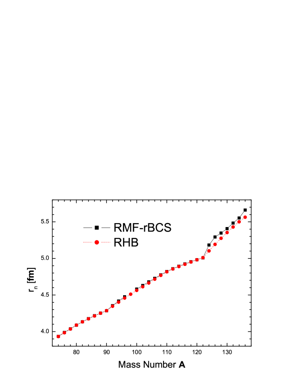
Figure 6: Root mean square neutron radii of even Zr isotopes as a function of the mass number A.

The behaviour of the nuclear radii close to the drip line is very sensitive to the relative occupancy of the loosely bound states and the low-lying narrow resonances with high angular momenta. Thus if the diffusivity of the Fermi sea is increasing the pairs scatter from the loosely bound states to the narrow resonances, which are more localized around the nucleus. Consequently the nuclear radii might decrease if the average pairing gap is increasing.

This effect can be also seen in the present calculations. In the RHB calculations the occupancy of the narrow resonances with high angular momenta is larger than in RMF-rBCS calculations. Accordingly, as seen in Figure 6, the RHB radii are smaller than in RMF-BCS calculations. This situation is quite general since in the RHB or HFB calculations, based on a big energy cut off, the Fermi sea is usually more diffuse than in rBCS-type calculations, even if the pairing correlation energies might be rather similar in the two calculations.

IV Conclusions

In this paper we discussed how the resonant states can be treated accurately in the RMF-BCS approach. The resonant states are described through the scattering states located in the vicinity of the resonance energies. These states are calculated by solving the RMF equations with scattering-type boundary conditions for the continuum spectrum. In the RMF-BCS equations the matrix elements of the pairing interaction involving resonant states are calculated by using the scattering states evaluated at the resonance energies and normalised inside a finite region close to the nucleus. The variation of the matrix elements of the pairing interaction due to the widths of the resonant states is taken into account by the derivative of the phase shift. This approximation scheme, used previously in non-relativistic HF-BCS calculations, is applied here for the neutron-rich Zr isotopes. It is shown that the sudden increase of the neutron radii close to the neutron drip line depends on a few resonant states close to the continuum threshold. Including into the RMF-BCS calculations only these resonant states one gets for the neutron radii and neutron separation energies practically the same results as in the more involved RHB calculations.

Acknowledgments We thank J. Meng for useful discussions on RHB calculations. One of us (N.S) gratefully acknowledges the COE Professorship Programme of Monkasho for suporting his visit to Osaka University, where this work was initiated, and the Swedish Programme for Cooperation in Research and Higher Education (STINT).

References

- (1) A. Bohr, B. Mottelson, and D. Pines, Phys. Rev. 110 (1958) 936.
- (2) S.T. Belyaev, A.V. Smirnov, S.V. Tolokonnikov, and S.A. Fayans, Sov. J. Nucl. Phys. 45 (1987), 783.
- (3) S.A. Fayans, S.V. Tolokonnikov, and D. Zawischa, Phys. Lett. B 491 (2000), 245.
- (4) A. Bulgac, preprint No. FT-194-1980, ICEFIZ- Bucharest; nucl-th/9907088.
- (5) M. Grasso, N. Sandulescu, Nguyen Van Giai, and R. J. Liotta, Phys. Rev. C64 (2001) 064321.
- (6) P. Ring and P. Schuck, The Nuclear Many-Body Problem (Springer-Verlag, Berlin, 1980)
- (7) P. Ring, Prog. Part. Nucl. Phys. 37 (1996) 193.
- (8) J. Meng and P. Ring, Phys. Rev. Lett 77 (1996) 3963
- (9) J. Dobaczewski, H. Flocard, and J. Treiner, Nucl. Phys. A 422 (1984), 103; J. Dobaczewski et al, Phys. Rev. C 53 (1996), 2809.
- (10) M. Grasso, Nguyen Van Giai, N. Sandulescu, Phys. Lett. B535 (2002) 103.
- (11) N Sandulescu, R. J. Liotta, R. Wyss, Phys. Lett. B392 (1997) 6; N. Sandulescu et al, Phys. Rev. C61 (2000) 044317.
- (12) N. Sandulescu, Nguyen Van Giai, R. J. Liotta, Phys. Rev. C61 (2000) 061301(R).
- (13) M. Del Estal, M. Centelles, X. Vinas, and S. K. Patra, Phys. Rev. C63 (2001) 044321.
- (14) P. -G. Reinhard, et al., Z. Phys. A323 (1986) 13.
- (15) A. B. Migdal, A. M. Perelemov, and V. S. Popov, Sov. J. Nucl. Phys. 14 (1971), 488.
- (16) H-J. Unger, Nucl. Phys. A104 (1967) 564
- (17) J. Meng and P. Ring, Phys. Rev. Lett. 80 (1998) 460
- (18) M. M. Sharma, M. A. Nagaranjan and P. Ring, Phys. Lett. B312 (1993) 377.
- (19) G. A. Lalazissis, J. Knig, and P. Ring, Phys. Rev C55 (1997) 540.
- (20) Y. Sugahara and H. Toki, Nucl. Phys. A579 (1994) 557.
- (21) G. Audi and A. H. Wapstra, Nucl. Phys. A595 (1995) 409