$\bm{\rho}$ meson photoproduction at low energies

Abstract

The $\sigma$-exchange and $f_{2}$-exchange mechanisms for $\rho$ meson photoproduction are re-examined. Then the commonly employed $\sigma$-exchange amplitude is revised by using the recent information from the analyses on the $\rho\to\pi^{0}\pi^{0}\gamma$ decay and the $\sigma NN$ coupling constant from Bonn potential. Instead of relying on the Pomeron-$f$ proportionality assumption, the $f_{2}$ meson exchange amplitude is established from an effective Lagrangian which is constructed from the tensor structure of the $f_{2}$ meson. Phenomenological information together with tensor meson dominance and vector meson dominance assumptions are used to estimate the $f_{2}$ coupling constants. As a first step to improve the current theoretical models, we have also explored the effects due to the un-correlated $2\pi$ exchange amplitude with $\pi N$ intermediate state. This leading-order $2\pi$ exchange amplitude can be calculated using the coupling constants determined from the study of pion photoproduction and the empirical width of $\rho\rightarrow\pi\pi$ decay. In comparing with the existing differential cross section data, we find that a model with the constructed $2\pi$, $\sigma$, and $f_{2}$ exchanges is comparable to the commonly used $\sigma$ exchange model in which the $\sigma$ coupling parameters are simply adjusted to fit the experimental data. We suggest that experimental verifications of the predicted single and double spin asymmetries in the small $|t|$ ($<2$ GeV²) region will be useful for distinguishing the two models and improving our understanding of the non-resonant amplitude of $\rho$ photoproduction. Possible further improvements of the model are discussed.

I Introduction

The recent experiments at Thomas Jefferson National Accelerator Facility (TJNAF) CLAS00 ; CLAS01 ; CLAS01b ; CLAS03 , GRAAL of Grenoble graal , and LEPS of SPring-8 leps are expected to provide new opportunities for studying the electromagnetic production of vector mesons at low energies. For example, the differential cross section data for $\rho$ photoproduction from the CLAS Collaboration at TJNAF show big differences with the old data of 1970’s CDGL76 ; BSYP78 in the large momentum-transfer ($|t|$) region at low energies, where one may learn about the $VNN$ couplings and other production mechanisms TLTS99 ; Lage00 ; OB01 ; Oh03 . Much more new data with similar high precisions will soon be available.

The study of vector meson photoproduction is expected to shed light on the resolution of the so-called ‘missing resonance’ problem CR00 ; OTL01 ; ZLB98c ; Zhao01 ; TL03 . On the other hand, it is well known that this can be achieved only when the nonresonant mechanisms are well understood OL02 ; PM02c . As a continuation of our effort in this direction OTL01 ; OL02 , we explore in this work the nonresonant mechanisms of $\rho$ photoproduction.

There exist some investigations of the nonresonant mechanisms for vector meson photoproduction. To account for the diffractive features of the data in small $t$ region at high energies, the Pomeron exchange model, as illustrated in Fig. 1(a), was developed. However, this model fails to describe the experimental observables at low energies. Indeed, meson exchanges (or secondary Reggeon exchanges) are found to be crucial in understanding the low energy data. In the case of $\omega$ photoproduction, it is well known that one-pion exchange is the most dominant process at low energies. For $\rho$ photoproduction, however, the situation is not clear. Generally, there are two scenarios which are based on either the $\sigma$ meson exchange model FS96 ; OTL00 or the $f_{2}$ exchange model Lage00 ; KV01a-KV02 . The $\sigma$ exchange model was motivated FS96 by the observation that the decay width of $\rho\to\pi\pi\gamma$ is much larger than the other radiative decays of the $\rho$ meson. It is further assumed that the $\pi\pi$ in the $\pi\pi\gamma$ channel can be modeled as a $\sigma$ meson so that the $\rho\sigma\gamma$ vertex can be defined and modeled for calculating the $\sigma$ exchange mechanism as illustrated in Fig. 1(b). In practice, the product of the coupling constants $g_{\rho\sigma\gamma}g_{\sigma NN}$ of this tree-diagram is adjusted to fit the cross section data of $\rho$ photoproduction at low energies. If we use $g_{\sigma NN}^{2}/4\pi\sim 8$ from Bonn potential MHE87 , we then find that the resulting $g_{\rho\sigma\gamma}$ will yield a decay width of $\rho^{0}\to\sigma\gamma$ an order of magnitude larger than the value extracted from the recent experimental decay width of $\rho^{0}\to\pi^{0}\pi^{0}\gamma$ GY01a ; BELN01 ; SND02 . Thus the dynamical interpretation of the commonly used $\sigma$ meson exchange model for $\rho$ meson photoproduction must be further examined theoretically.

In this work, we would like to take a different approach to account for the exchange of $\pi\pi$ in $\rho$ photoproduction. First, the commonly employed $\sigma$-exchange amplitude is revised by using the coupling constant $g_{\sigma NN}$ from Bonn potential and $g_{\rho\sigma\gamma}$ from the recent experimental decay width of $\rho^{0}\to\pi^{0}\pi^{0}\gamma$ with the assumption FS96 that $\pi^{0}\pi^{0}$ in this decay is strongly correlated and can be approximated as a $\sigma$ particle. This is our starting point of developing a new model which is more consistent with the existing meson-exchange models for $NN$ scattering MHE87 , $\pi N$ scattering, and pion photoproduction SL96 . We then consider the consequence of the strong $\rho\to\pi^{+}\pi^{-}$ decay which accounts for almost the entire decay width of the $\rho$ meson. With the empirical value of the $\rho$ meson decay width, one can define the $\rho\pi\pi$ vertex, which then leads naturally to the ‘uncorrelated’ two-pion exchange mechanism illustrated in Fig. 2 with $M=\pi$ in the intermediate state. A more complete calculation of un-correlated $2\pi$-exchange contributions to $\rho$ photoproduction should also include other intermediate states such as $\omega N$ and $\pi\Delta$. However, the contributions from these intermediate states involve propagation of two or three pions and must be considered along with other multi-pion exchange mechanisms (such as the crossed diagrams due to the interchange of $\gamma$ and $\rho$ lines in Fig. 2). Obviously, this is a much more complex task and will not be attempted in this exploratory investigation. Our calculation of $2\pi$-exchange will be detailed in Section II.F.

The $f_{2}$ exchange model for $\rho$ photoproduction was motivated by the results from the analyses of $pp$ scattering data at low energies DL92 . In the study of $pp$ scattering the dominant secondary Regge trajectory is represented by the $f$ trajectory, and the idea of Pomeron-$f$ proportionality had been used to model the Pomeron couplings using the $f_{2}$ couplings until 1970’s Freu62 ; Freu71 ; CGZ71 ; KS73 before the advent of the soft Pomeron model by Donnachie and Landshoff DL84 . By considering the role of the $f$ trajectory in $pp$ scattering, it is natural to consider the $f_{2}$ exchange model for vector meson photoproduction. However, the $f_{2}$ exchange model developed in Refs. Lage00 ; KV01a-KV02 for $\rho$ photoproduction made use of the Pomeron-$f$ proportionality in the reverse direction. Namely, they assume that the structure of the $f_{2}$ couplings are the same as that of the soft Pomeron exchange model. Thus the $f_{2}$ tensor meson was treated as a $C=+1$ isoscalar photon, i.e., a vector particle. In addition, the fit to the data is achieved by introducing an additional adjustable parameter to control the strength of the $f_{2}$ coupling Lage00 . This is obviously not very satisfactory and leaves a room for improvement.

Instead of relying on the Pomeron-$f$ proportionality assumption, the $f_{2}$ meson exchange amplitude is evaluated in this work starting with an effective Lagrangian which is constructed from the tensor structure of the $f_{2}$ meson. Phenomenological information together with tensor meson dominance and vector meson dominance assumptions are used to estimate the $f_{2}$ coupling constants. With this, we then explore the extend to which the $\rho$ photoproduction data can be described by a model that includes this newly constructed $f_{2}$ exchange amplitude together with the revised $\sigma$-exchange amplitude and the un-correlated $2\pi$-exchange amplitudes discussed above.

This paper is organized as follows. In Section II, we explicitly define the amplitudes for the considered $\rho$ photoproduction mechanisms, including the Pomeron exchange, $\sigma$ exchange, pseudoscalar meson exchanges, $s$- and $u$-channel nucleon terms, and the newly constructed $f_{2}$ exchange. The $2\pi$ exchange amplitudes are then given to complete our model construction. The numerical results are presented in Section III. For comparison, we consider two models. Both models contain the $s$- and $u$-channel nucleon terms and the exchanges of Pomeron, $\pi$, and $\eta$. In addition, the first model includes the $\sigma$ exchange with free parameters to fit the data following Refs. FS96 ; OTL00 , while the second model contains the two-pion, $\sigma$, and $f_{2}$ exchanges, where the parameters of the $\sigma$ exchange are fixed by Bonn potential and $\rho\to\pi^{0}\pi^{0}\gamma$ decay. We explore the extent to which these two rather different models can be distinguished by examining the differential cross sections and spin asymmetries. Section IV contains a summary and discussions. The details on the $f_{2}$ interactions with the photon and hadrons are given in Appendix for completeness.

II Models for $\bm{\rho}$ photoproduction

In this Section, we discuss possible production mechanisms for $\gamma p\to\rho p$. We first discuss single particle exchanges as depicted in Fig. 1. Then the $2\pi$ exchange model will be constructed. Each of the considered production amplitude, as illustrated in Fig. 1, can be written as

$$T_{fi}=\varepsilon_{\mu}^{*}(V)\mathcal{M}^{\mu\nu}\varepsilon_{\nu}(\gamma),$$ (1)

where $\varepsilon_{\mu}(V)$ and $\varepsilon_{\nu}(\gamma)$ are the polarization vectors of the vector meson and the photon, respectively. We denote the four-momenta of the initial nucleon, final nucleon, incoming photon, and outgoing vector meson by $p$, $p^{\prime}$, $k$, and $q$, respectively. The Mandelstam variables are $s=W^{2}=(k+p)^{2}$, $t=(p-p^{\prime})^{2}$, and $u=(p-q)^{2}$.

Figure 1: Models for $\rho$ photoproduction. (a,b) $t$-channel Pomeron and one-meson exchanges ($M=f_{2},\pi,\eta,\sigma$), (c,d) $s$- and $u$-channel nucleon pole terms.

II.1 Pomeron exchange

We first consider the Pomeron exchange depicted in Fig. 1(a). In this process, the incoming photon first converts into a $q\bar{q}$ pair, which interacts with the nucleon by the Pomeron exchange before forming the outgoing vector meson. The quark-Pomeron vertex is obtained by the Pomeron-photon analogy DL84 , which treats the Pomeron as a $C=+1$ isoscalar photon, as suggested by a study of nonperturbative two-gluon exchanges LN87 . We then have DL84 ; LM95 ; PL97 ; TOYM98

$$\mathcal{M}^{\mu\nu}_{\mathbb{P}}=G_{\mathbb{P}}(s,t)\mathcal{T}^{\mu\nu}_{\mathbb{P}},$$ (2)

with

$$\mathcal{T}^{\mu\nu}_{\mathbb{P}}=i12\sqrt{4\pi\alpha_{\rm em}}\frac{M_{V}^{2}\beta_{q}\beta_{q^{\prime}}}{f_{V}}\frac{1}{M_{V}^{2}-t}\left(\frac{2\mu_{0}^{2}}{2\mu_{0}^{2}+M_{V}^{2}-t}\right)F_{1}(t)\bar{u}(p^{\prime})\{k\!\!\!/\,g^{\mu\nu}-k^{\mu}\gamma^{\nu}\}u(p),$$ (3)

where $\alpha_{\rm em}=e^{2}/4\pi$ and $F_{1}$ is the isoscalar electromagnetic form factor of the nucleon,

$$F_{1}(t)=\frac{4M_{N}^{2}-2.8t}{(4M_{N}^{2}-t)(1-t/0.71)^{2}},$$ (4)

with $t$ in GeV². The proton and vector meson masses are represented by $M_{N}$ and $M_{V}$, respectively. ($M_{V}=M_{\rho}$ in our case.)

The Regge propagator for the Pomeron in Eq. (2) reads

$$G_{\mathbb{P}}=\left(\frac{s}{s_{0}}\right)^{\alpha_{P}(t)-1}\exp\left\{-\frac{i\pi}{2}\left[\alpha_{P}(t)-1\right]\right\}.$$ (5)

The Pomeron trajectory is taken to be the usual form $\alpha_{P}(t)=1.08+\alpha^{\prime}_{P}t$ with $\alpha^{\prime}_{P}=1/s_{0}=0.25$ GeV^-2 DL84 . In Eq. (3), $f_{V}$ is the vector meson decay constant: $f_{\rho}=5.33$, $f_{\omega}=15.2$, and $f_{\phi}=13.4$. The coupling constants $\beta_{u}=\beta_{d}=2.07$ GeV^-1, $\beta_{s}=1.60$ GeV^-1, and $\mu_{0}^{2}=1.1$ GeV² are chosen to reproduce the total cross section data at high energies, $E_{\gamma}\geq 10$ GeV, where the total cross section of vector meson photoproductions are completely dominated by the Pomeron exchange. For $\rho$ photoproduction, we set $\beta_{q}=\beta_{q^{\prime}}=\beta_{u}=\beta_{d}$.

II.2 $\bm{\sigma}$ meson exchange

The $\sigma$ meson exchange model advocated by Friman and Soyeur FS96 is based on the observation that $\Gamma(\rho\to\pi\pi\gamma)$ is the largest among all $\rho$ meson radiative decays, which leads to the assumption that the $\rho$ photoproduction process at low energies is dominated by the exchange of $2\pi$. The $2\pi$ is then effectively represented by a $\sigma$ meson. The effective Lagrangian for this model reads FS96 ; TLTS99 ; OTL00

$$\mathcal{L}_{\sigma}=\frac{eg_{\rho\sigma\gamma}}{M_{\rho}}\left(\partial^{\mu}\rho^{\nu}\partial_{\mu}A_{\nu}-\partial^{\mu}\rho^{\nu}\partial_{\nu}A_{\mu}\right)\sigma+g_{\sigma NN}\bar{N}\sigma N,$$ (6)

where $\rho_{\mu}$ is the $\rho^{0}$ meson field and $A_{\mu}$ the photon field. The resulting $\sigma$ meson exchange amplitude is

$$\mathcal{M}^{\mu\nu}_{\sigma}=\frac{eg_{\rho\sigma\gamma}g_{\sigma NN}}{M_{\rho}}\frac{1}{t-M_{\sigma}^{2}}\left(k\cdot qg^{\mu\nu}-k^{\mu}q^{\nu}\right)\bar{u}(p^{\prime})u(p)F_{\sigma NN}(t)F_{\rho\sigma\gamma}(t),$$ (7)

where

$$F_{\sigma NN}(t)=\frac{\Lambda_{\sigma}^{2}-M_{\sigma}^{2}}{\Lambda_{\sigma}^{2}-t},\qquad F_{\rho\sigma\gamma}(t)=\frac{\Lambda_{\rho\sigma\gamma}^{2}-M_{\sigma}^{2}}{\Lambda_{\rho\sigma\gamma}^{2}-t}$$ (8)

are the form factors. The cutoff parameters of the form factors and the product of coupling constants $g_{\rho\sigma\gamma}g_{\sigma NN}$ are adjusted to fit the $\rho$ photoproduction data at low energies. It was found FS96 ; OTL00 that

$$M_{\sigma}=0.5\mbox{ GeV},\qquad g^{2}_{\sigma NN}/4\pi=8.0,\qquad g_{\rho\sigma\gamma}=3.0,$$

$$\Lambda_{\sigma}=1.0\mbox{ GeV},\qquad\Lambda_{\rho\sigma\gamma}=0.9\mbox{ GeV}.$$ (9)

The resulting $\sigma$ mass parameter is close to the value $M_{\sigma}=0.55\sim 0.66$ GeV of Bonn potential MHE87 . If we further take the value $g^{2}_{\sigma NN}/4\pi=8.3\sim 10$ from Bonn potential, we then find that the resulting $g_{\rho\sigma\gamma}$ is close to the values from the QCD sum rules, $g_{\rho\sigma\gamma}(\mbox{\small QCDSR})=3.2\pm 0.6$ GY01 or $2.2\pm 0.4$ AOS02 . However such a large value of $g_{\rho\sigma\gamma}$ corresponds to the $\rho\rightarrow\sigma\gamma(\to\pi^{0}\pi^{0}\gamma)$ decay width that is much larger than the empirical value of $\Gamma(\rho^{0}\to\pi^{0}\pi^{0}\gamma)$ BELN01 ; SND02 . If we accept the empirically estimated, but model-dependent value of SND experiment SND02 , $\mbox{BR}(\rho\to\sigma\gamma)=(1.9\stackrel{{\scriptstyle+0.9}}{{\mbox{\scriptsize$-0.8$}}}\pm 0.4)\times 10^{-5}$, which gives $\Gamma(\rho\to\sigma\gamma)\approx 2.83$ keV, we get

$$|g_{\rho\sigma\gamma}|\approx 0.25,$$ (10)

since the Lagrangian (6) gives

$$\Gamma(\rho\to\sigma\gamma)=\frac{\alpha_{\rm em}g^{2}_{\rho\sigma\gamma}}{24M_{\rho}^{5}}\left(M_{\rho}^{2}-M_{\sigma}^{2}\right)^{3}.$$ (11)

This value is smaller than that of Eq. (9) by an order of magnitude. Therefore, the $\sigma$ exchange model suffers from the big uncertainty of $g_{\rho\sigma\gamma}$, which is under debate BELN01 ; GY01a ; SND02 ; BE03 ; OK03 . Furthermore, there is no clear particle identification of a $\sigma$ particle and the use of $\sigma$ exchange in defining $NN$ potential has been seriously questioned. Thus it is possible that the $\sigma$ exchange may not be the right major mechanism for $\rho$ photoproduction.

II.3 Pseudoscalar meson exchanges

The $\pi$ and $\eta$ meson exchanges are also allowed for $\rho$ photoproduction, although their contributions are known to be not important. They are calculated from

$$\mathcal{L}_{\rho\gamma\varphi} = \frac{eg_{\rho\gamma\varphi}}{M_{V}}\epsilon^{\mu\nu\alpha\beta}\partial_{\mu}\rho_{\nu}\partial_{\alpha}A_{\beta}\varphi,$$

$$\mathcal{L}_{\varphi NN} = \frac{g_{\varphi NN}}{2M_{N}}\bar{N}\gamma^{\mu}\gamma_{5}\partial_{\mu}\varphi N,$$ (12)

where $\varphi=\pi^{0},\eta$. The coupling constants $g_{\rho\gamma\varphi}$ are fixed by the $\rho\to\varphi\gamma$ decay widths

$$\Gamma(\rho\to\varphi\gamma)=\frac{\alpha_{\rm em}g_{\rho\gamma\varphi}^{2}}{24M_{V}^{5}}(M_{V}^{2}-M_{\varphi}^{2})^{3}.$$ (13)

Using the experimental data PDG02 , $\Gamma(\rho^{0}\to\pi^{0}\gamma)_{\rm expt.}=121\pm 31$ keV and $\Gamma(\rho^{0}\to\eta\gamma)_{\rm expt.}=62\pm 17$ keV, we get

$$g_{\rho\gamma\pi}=0.756,\qquad g_{\rho\gamma\eta}=1.476.$$ (14)

This also gives $g_{\omega\gamma\pi}=1.843$ and $g_{\omega\gamma\eta}=0.414$. We use $g_{\pi NN}^{2}/4\pi=14.3$ and the SU(3) relation to get $g_{\eta NN}^{2}/4\pi=0.99$. Although there are other estimates on the value of $g_{\eta NN}$ reported in the literature, the role of the $\eta$ exchange is much suppressed in $\rho$ photoproduction and the dependence of our results on $g_{\eta NN}$ is negligible.

The pseudoscalar meson exchange amplitude, Fig. 1(b), calculated from the Lagrangian (12) reads

$$\mathcal{M}_{\varphi}^{\mu\nu}=\frac{ieg_{\rho\gamma\varphi}g_{\varphi NN}}{2M_{N}M_{V}}\frac{1}{t-M_{\varphi}^{2}}\epsilon^{\mu\nu\alpha\beta}q_{\alpha}k_{\beta}\bar{u}(p^{\prime})(p\!\!\!/-p\!\!\!/^{\prime})\gamma_{5}u(p)F_{\varphi NN}(t)F_{\rho\varphi\gamma}(t),$$ (15)

where the form factors are

$$F_{\varphi NN}(t)=\frac{\Lambda_{\varphi}^{2}-M_{\varphi}^{2}}{\Lambda_{\varphi}^{2}-t},\qquad F_{\rho\varphi\gamma}(t)=\frac{\Lambda_{\rho\varphi\gamma}^{2}-M_{\varphi}^{2}}{\Lambda_{\rho\varphi\gamma}^{2}-t}.$$ (16)

We use $\Lambda_{\pi}=0.6$ GeV, $\Lambda_{\rho\pi\gamma}=0.77$ GeV, $\Lambda_{\eta}=1.0$ GeV, and $\Lambda_{\rho\eta\gamma}=0.9$ GeV FS96 ; OTL01 .

II.4 Nucleon pole terms

The $s$- and $u$-channel nucleon terms, Figs. 1(c,d), are calculated from

$$\mathcal{L}_{\gamma pp} = -e\bar{N}\left[A_{\mu}\gamma^{\mu}-\frac{\kappa_{p}}{2M_{N}}\sigma_{\mu\nu}\partial^{\nu}A^{\mu}\right]N,$$

$$\mathcal{L}_{\rho pp} = -\frac{g_{\rho NN}}{2}\bar{N}\left[\rho^{\mu}\gamma_{\mu}-\frac{\kappa_{\rho}}{2M_{N}}\sigma_{\mu\nu}\partial^{\nu}\rho^{\mu}\right]N.$$ (17)

The resulting production amplitude is

$$\mathcal{M}_{N}^{\mu\nu} = \frac{eg_{\rho NN}}{2}\bar{u}(p^{\prime})\biggl{[}\Gamma^{\mu}_{V}(q)\frac{p\!\!\!/+k\!\!\!/+M_{N}}{s-M_{N}^{2}}\Gamma_{\gamma}^{\nu}(k)F_{N}(s)$$ (18)

$$\qquad\mbox{}+\Gamma^{\nu}_{\gamma}(k)\frac{p\!\!\!/-q\!\!\!/+M_{N}}{u-M_{N}^{2}}\Gamma_{V}^{\mu}(q)F_{N}(u)\biggr{]}u(p),$$

where

$$\Gamma^{\mu}_{V}=\gamma^{\mu}-i\frac{\kappa_{\rho}}{2M_{N}}\sigma^{\mu\nu}q_{\nu},\qquad\Gamma^{\mu}_{\gamma}=\gamma^{\mu}+i\frac{\kappa_{p}}{2M_{N}}\sigma^{\mu\nu}k_{\nu}.$$ (19)

The form factor has the form PJ91

$$F_{N}(r)=\frac{\Lambda_{N}^{4}}{\Lambda_{N}^{4}+(r-M_{N}^{2})^{2}},$$ (20)

with $\Lambda_{N}=0.5$ GeV taken from Refs. OTL01 ; TLTS99 . This choice of the nucleon form factor leads to a satisfactory explanation of the steep rise of the differential cross sections with increasing $|t|$ in terms of the $u$-channel nucleon term [Fig. 1(d)].

Because $F_{N}(s)\neq F_{N}(u)$, the above amplitude does not satisfy the gauge invariance. In order to restore the gauge invariance, we project out the gauge non-invariant terms as

$$\Gamma_{V}^{\mu}\to\Gamma_{V}^{\mu}-\frac{k^{\mu}}{k\cdot q}\,q\cdot\Gamma_{V},\qquad\Gamma_{\gamma}^{\mu}\to\Gamma_{\gamma}^{\mu}-\frac{q^{\mu}}{k\cdot q}\,k\cdot\Gamma_{\gamma}.$$ (21)

For the $\rho NN$ coupling constants, we take the values determined in the analyses of pion photoproduction and $\pi N$ scattering SL96 :

$$g_{\rho NN}=6.2,\qquad\kappa_{\rho}=1.0,$$ (22)

and the anomalous magnetic moment of the nucleon is $\kappa_{p}=1.79$.

II.5 $\bm{f_{2}}$ meson exchange

We now discuss the exchange of the $f_{2}(1270)$ tensor meson, which has quantum numbers $I^{G}(J^{PC})=0^{+}(2^{++})$. The mass and decay width of the $f_{2}(1270)$ are $M_{f}=1275.4\pm 1.2$ MeV and $\Gamma(f_{2})=185.1\stackrel{{\scriptstyle+3.4}}{{\mbox{\scriptsize$-2.6$}}}$ MeV PDG02 . Because of its quantum numbers, it has been once suggested as a candidate for the Pomeron. But this assumption violates the duality with the $a_{2}$ trajectory which includes $I^{G}(J^{PC})=1^{-}(2^{++})$ state and it is now believed that the $f_{2}$ does not lie on the Pomeron trajectory.

In the approach of Ref. Lage00 , the $f_{2}$ is treated as a $C=+1$ isoscalar photon just like the Pomeron. This leads to a Regge amplitude of the following form

$$\mathcal{M}^{\mu\nu}_{f_{2}}=\kappa_{f_{2}}G_{f_{2}}(s,t)\mathcal{T}^{\mu\nu}_{\mathbb{P}},$$ (23)

where

$$G_{f_{2}}(s,t)=\left(\frac{s}{s_{1}}\right)^{\alpha_{f_{2}}(t)-1}\frac{(1+\exp[-i\pi\alpha_{f_{2}}(t)])\pi\alpha^{\prime}_{f_{2}}}{2\sin[\pi\alpha_{f_{2}}(t)]\,\Gamma[\alpha_{f_{2}}(t)]},$$ (24)

with $s_{1}=1/\alpha^{\prime}_{f_{2}}\approx 1$ GeV², while the form of $\mathcal{T}^{\mu\nu}_{\mathbb{P}}$ is the same as given in Eq. (3). The $f_{2}$ trajectory is linearly approximated as $\alpha_{f_{2}}(t)\approx 0.47+0.89t$ DL92 ; KV01a-KV02 . In order to control the strength of the $f_{2}$ couplings to the hadrons, a free parameter $\kappa_{f_{2}}$ was introduced Lage00 and adjusted to fit the $\rho$ photoproduction data at low energies.

In this paper, we depart from this Regge parameterization and construct an $f_{2}$ exchange model solely based on the tensor structure of the $f_{2}$ meson. We will use the experimental data associated with the $f_{2}$ meson, the tensor meson dominance, and vector meson dominance assumptions to fix the $f_{2}$ coupling constants, such that the strength of the resulting $f_{2}$ exchange amplitude is completely fixed in this investigation. Following Refs. Gold68 ; PSMM73 , the effective Lagrangian accounting for the tensor structure of the $f_{2}NN$ interaction is written as

$$\mathcal{L}_{fNN}=-2i\frac{G_{fNN}}{M_{N}}\bar{N}(\gamma_{\mu}\partial_{\nu}+\gamma_{\nu}\partial_{\mu})Nf^{\mu\nu}+4\frac{F_{fNN}}{M_{N}}\partial_{\mu}\bar{N}\partial_{\nu}Nf^{\mu\nu},$$ (25)

where $f^{\mu\nu}$ is the $f_{2}$ meson field. This gives the following form of the $fNN$ vertex function,

$$V_{be,d}=-\epsilon^{\mu\nu}\bar{u}(p_{d})\left\{\frac{G_{fNN}}{M_{N}}\left[\Sigma_{\mu}\gamma_{\nu}+\gamma_{\nu}\Sigma_{\mu}\right]+\frac{F_{fNN}}{M_{N}^{2}}\Sigma_{\mu}\Sigma_{\nu}\right\}u(p_{b}),$$ (26)

where $\Sigma_{\mu}=(p_{b}+p_{d})_{\mu}$, $p_{b}$ and $p_{d}$ are the incoming and outgoing nucleon momentum, respectively, and $\epsilon^{\mu\nu}$ is the polarization tensor of the $f_{2}$ meson.

The coupling constants associated with the $f_{2}$ meson were first estimated by using the dispersion relations to analyze the backward $\pi N$ scattering Gold68 and the $\pi\pi\to N\bar{N}$ partial-wave amplitudes. The results are summarized in Table 1. Note that the value estimated based on the tensor-meson dominance Renn70 is much smaller than the empirical values. (See Appendix for details.)

${G_{fNN}^{2}}/{4\pi}$	$F_{fNN}/G_{fNN}$
$1.12$	—	Ref. Gold68
$3.31$	$\approx 0$	Ref. ASS70
$3.31\pm 0.63$	$0.06\pm 0.17$	Ref. Engels70
$4.0\pm 1.0$	$0.00\pm 0.07$	Ref. Hede77
$2.2\pm 0.9$	$0.6\pm 0.9$	Ref. BK77
$0.38\pm 0.04$	$\approx 0$	Ref. Renn70

Table 1: Estimates on the $fNN$ coupling constants, $G_{fNN}$ and $F_{fNN}$, using $\pi N$ dispersion relations. The values are compared with the prediction of tensor meson dominance Renn70 .

The most general form for the $fV\gamma$ vertex satisfying gauge invariance reads Renn71

$$\langle\gamma(k)V(k^{\prime})|f_{2}\rangle=\frac{1}{M_{f}}\epsilon^{\kappa}\epsilon^{\prime\lambda}f^{\mu\nu}A_{\kappa\lambda\mu\nu}^{fV\gamma}(k,k^{\prime}),$$ (27)

where $\epsilon$ and $\epsilon^{\prime}$ are the polarization vectors of the photon and the vector meson, respectively, and

$$A^{fV\gamma}_{\kappa\lambda\mu\nu}(k,k^{\prime}) = \frac{f_{fV\gamma}}{M_{f}^{3}}\left[g_{\kappa\lambda}(k\cdot k^{\prime})-k^{\prime}_{\kappa}k_{\lambda}\right](k-k^{\prime})_{\mu}(k-k^{\prime})_{\nu}$$ (28)

$$\mbox{}+g_{fV\gamma}[g_{\kappa\lambda}(k-k^{\prime})_{\mu}(k-k^{\prime})_{\nu}+g_{\lambda\mu}k^{\prime}_{\kappa}(k-k^{\prime})_{\nu}+g_{\lambda\nu}k^{\prime}_{\kappa}(k-k^{\prime})_{\mu}$$

$$\mbox{}\qquad-g_{\kappa\mu}k_{\lambda}(k-k^{\prime})_{\nu}-g_{\kappa\nu}k_{\lambda}(k-k^{\prime})_{\mu}-2k\cdot k^{\prime}(g_{\kappa\mu}g_{\lambda\nu}+g_{\kappa\nu}g_{\lambda\mu})].$$

The tensor meson dominance assumption together with the vector meson dominance gives Renn71

$$f_{fV\gamma}=0\qquad\mbox{ and }\qquad g_{fV\gamma}=\frac{e}{f_{V}}G_{fVV},$$ (29)

where

$$G_{fVV}=G_{f\pi\pi}=5.76.$$ (30)

Here $G_{f\pi\pi}$ is determined from the decay width of $f_{2}\to\pi\pi$. The details on the $f_{2}$ interactions with the photon and hadrons, and tensor meson dominance are given in Appendix.

With the above formulas, it is straightforward to obtain the production amplitude as

$$\mathcal{M}^{\mu\nu}_{f_{2}}=-\bar{u}(p)\Gamma^{\alpha\beta}(p,p^{\prime})u(p)\frac{P_{\alpha\beta;\rho\sigma}}{(p-p^{\prime})^{2}-M_{f}^{2}}V^{\rho\sigma;\nu\mu}(k,q)F_{fNN}(t)F_{fV\gamma}(t),$$ (31)

where

$$\Gamma_{\alpha\beta}(p,p^{\prime}) = \frac{G_{fNN}}{M_{N}}\left[(p+p^{\prime})_{\alpha}\gamma_{\beta}+(p+p^{\prime})_{\beta}\gamma_{\alpha}\right]+\frac{F_{fNN}}{M_{N}^{2}}(p+p^{\prime})_{\alpha}(p+p^{\prime})_{\beta},$$

$$P_{\alpha\beta;\rho\sigma} = \frac{1}{2}(\bar{g}_{\alpha\rho}\bar{g}_{\beta\sigma}+\bar{g}_{\alpha\sigma}\bar{g}_{\beta\rho})-\frac{1}{3}\bar{g}_{\alpha\beta}\bar{g}_{\rho\sigma},$$

$$V^{\rho\sigma;\nu\mu}(k,q) = \frac{f_{fV\gamma}}{M_{f}^{4}}\left[-g_{\mu\nu}(k\cdot q)+q_{\nu}k_{\mu}\right](k+q)_{\rho}(k+q)_{\sigma}$$ (32)

$$\mbox{}+\frac{g_{fV\gamma}}{M_{f}}\biggl{[}g_{\mu\nu}(k+q)_{\rho}(k+q)_{\sigma}-g_{\mu\rho}q_{\nu}(k+q)_{\sigma}-g_{\mu\sigma}q_{\nu}(k+q)_{\rho}$$

$$\mbox{}\qquad-g_{\nu\rho}k_{\mu}(k+q)_{\sigma}-g_{\nu\sigma}k_{\mu}(k+q)_{\rho}+2k\cdot q(g_{\nu\rho}g_{\mu\sigma}+g_{\nu\sigma}g_{\mu\rho})\biggr{]},$$

and

$$\bar{g}_{\mu\nu}=-g_{\mu\nu}+\frac{(p-p^{\prime})_{\mu}(p-p^{\prime})_{\nu}}{M_{f}^{2}}.$$ (33)

The form factors are chosen as

$$F_{fNN}(t)=\frac{\Lambda_{fNN}^{2}-M_{f_{2}}^{2}}{\Lambda_{fNN}^{2}-t},\qquad F_{fV\gamma}(t)=\frac{\Lambda_{fV\gamma}^{2}-M_{f_{2}}^{2}}{\Lambda_{fV\gamma}^{2}-t},$$ (34)

where the cutoff parameters will be discussed in Sect. III. The relative phases among $f_{2}$ couplings are fixed by tensor meson dominance.

II.6 $\bm{2\pi}$ exchange

Figure 2: $2\pi$ exchange in $\rho$ photoproduction. The intermediate meson state ($M$) includes $\pi$, and the baryon ($B$) includes the nucleon.

In this subsection, we discuss the $2\pi$ exchange for $\rho$ photoproduction as shown in Fig. 2. We only consider the contribution from setting the intermediate state $(MB)=(\pi N)$. As discussed in Section I, the contributions from other intermediate states like $\pi\Delta$ and $\omega N$ involve propagation of two or three pions and hence are neglected along with the other multi-meson exchange amplitudes in this exploratory investigation.

We compute the loop amplitude of Fig. 2 by making use of the method of Sato and Lee SL96 , which gives

$$T_{\rm loop}=\int d^{3}{\bf q}^{\prime}\left[\varepsilon(\gamma)\cdot B_{\gamma N,MN}({\bf k},{\bf q}^{\prime};E)\right]G_{MN}({\bf q}^{\prime},E)\left[\varepsilon^{*}(V)\cdot V_{MN,\rho N}({\bf q}^{\prime},{\bf q}:E)\right],$$ (35)

where

$$G_{MN}({\bf q}^{\prime},E)=\frac{1}{E-E_{N}(q^{\prime})-E_{M}(q^{\prime})+i\epsilon}.$$ (36)

Obviously, $B_{\gamma N,MN}$ and $V_{MN,\rho N}$ are the one-pion-exchange amplitudes illustrated in Fig. 2. We only consider $(MN)=(\pi N)$ intermediate state in this paper.

Equation (35) can be rewritten as

$$T_{\rm loop} = \mathcal{P}\int d^{3}{\bf q}^{\prime}\frac{\varepsilon^{*}(V)\cdot V({\bf q}^{\prime},{\bf q})\,\varepsilon(\gamma)\cdot B({\bf k},{\bf q}^{\prime})}{W-E_{B}(q^{\prime})-E_{M}(q^{\prime})}$$ (37)

$$\mbox{}-i\int d\Omega_{k_{t}}\,\rho_{BM}({\bf k}_{t})\,\varepsilon^{*}(V)\cdot V({\bf k}_{t},{\bf q})\,\varepsilon(\gamma)\cdot B({\bf k},{\bf k}_{t})\,\theta(W-M_{M}-M_{B}),$$

where the subscripts of $V$ and $B$ are understood. Here $\theta(x)$ is the step function and

$$\rho_{BM}(k)=\frac{\pi kE_{B}(k)E_{M}(k)}{E_{B}(k)+E_{M}(k)},$$ (38)

where $E_{B}(k)$ and $E_{M}(k)$ are the energies of the intermediate baryon and meson with momentum ${\bf k}$. Through the on-shell condition $W=E_{B}(k_{t})+E_{M}(k_{t})$, $k_{t}$ is determined as

$$k_{t}=\frac{1}{2W}\sqrt{\lambda(W^{2},M_{M}^{2},M_{B}^{2})},$$ (39)

where

$$\lambda(x,y,z)=x^{2}+y^{2}+z^{2}-2(xy+yz+zx).$$ (40)

For the considered $(MN)=(\pi N)$ case, the one-pion-exchange amplitudes $B_{\gamma N,\pi N}$ and $V_{\pi N,\rho N}$ in Eq.(35) can be calculated from

$$\mathcal{L}_{\gamma\pi\pi} = e\left[\partial^{\mu}\bm{\pi}\times\bm{\pi}\right]_{3}A_{\mu},$$

$$\mathcal{L}_{\rho\pi\pi} = g_{\rho\pi\pi}\bm{\rho}_{\mu}\cdot\left(\bm{\pi}\times\partial^{\mu}\bm{\pi}\right),$$

$$\mathcal{L}_{\pi NN} = \frac{g_{\pi NN}}{2M_{N}}\bar{N}\gamma^{\mu}\gamma_{5}\bm{\tau}\cdot\partial_{\mu}\bm{\pi}N.$$ (41)

The coupling constant $g_{\rho\pi\pi}$ is determined from the decay width $\Gamma(\rho\to\pi\pi)$, which reads

$$\Gamma(\rho\to\pi\pi)=\frac{g_{\rho\pi\pi}^{2}}{48\pi M_{\rho}^{2}}\left(M_{\rho}^{2}-4M_{\pi}^{2}\right)^{3/2}.$$ (42)

Using $\Gamma(\rho^{0}\to\pi^{+}\pi^{-})=150.7$ MeV PDG02 , we obtain

$$g_{\rho\pi\pi}=6.04.$$ (43)

Then the $2\pi$-exchange transition amplitude with intermediate $\pi N$ channel reads

$$\widetilde{\mathcal{M}}_{\pi N}^{\mu\nu} \equiv V^{\mu}(q^{\prime},q)B^{\nu}(k,q^{\prime})$$ (44)

$$= \frac{1}{(2\pi)^{3}}\frac{M_{N}}{E_{N}(p_{B})}\frac{1}{2E_{\pi}(q^{\prime})}\frac{eg_{\rho\pi\pi}g_{\pi NN}^{2}}{4M_{N}^{3}}(q^{\prime}-p_{B}+p^{\prime})^{\mu}(p_{B}-p-q^{\prime})^{\nu}$$

$$\mbox{}\times\frac{1}{(p_{B}-p)^{2}-M_{\pi}^{2}}\frac{1}{(p_{B}-p^{\prime})^{2}-M_{\pi}^{2}}\bar{u}(p^{\prime})\Gamma u(p),$$

where

$$\Gamma=(p\!\!\!/^{\prime}-p_{B}\!\!\!\!\!\!/\ \ )\left(p_{B}\!\!\!\!\!\!/\ \ -M_{N}\right)(p_{B}\!\!\!\!\!\!/\ \ -p\!\!\!/).$$ (45)

The loop integration must be regularized by introducing form factors. We include the form factors for each vertices. In addition, we also introduce the form factor to take into account the off-shell-ness of the intermediate states,

$$F_{\ell}({\bf q}^{\prime})=\left(\frac{\Lambda_{\ell}^{2}+{\bf k}_{t}^{2}}{\Lambda_{\ell}^{2}+{\bf q}^{\prime 2}}\right)^{2}.$$ (46)

Thus the final form of the form factor is

$$F=F_{\ell}({\bf q}^{\prime})F_{\rho\pi\pi}(t_{1})F_{\rho\pi\pi}(t_{2})F_{\pi NN}(t_{1})F_{\pi NN}(t_{2}),$$ (47)

where

$$F_{\rho\pi\pi}(t)=\frac{\Lambda_{\rho\pi\pi}^{2}-M_{\pi}^{2}}{\Lambda_{\rho\pi\pi}^{2}-t},\qquad F_{\pi NN}(t)=\frac{\Lambda_{\pi NN}^{2}-M_{\pi}^{2}}{\Lambda_{\pi NN}^{2}-t},$$ (48)

and $t_{1}=(p_{B}-p)^{2}$ and $t_{2}=(p_{B}-p^{\prime})^{2}$. Here the inclusion of $F_{\rho\pi\pi}(t_{1})$ implies the vector meson dominance assumption. The cutoff parameters will be discussed in Sect. III.

We now comment on the loop calculation described above. We do not consider the crossed diagrams of Fig. 2, since such diagrams include three-particle intermediate states and hence are of higher-order effects which are neglected in this exploratory study. However by neglecting the crossed diagrams, the resulting amplitude does not satisfy gauge invariance. In this study, therefore, we restore gauge invariance of the amplitude (44) by projecting out the gauge non-invariant terms as TOYM98

$$\widetilde{\mathcal{M}}^{\mu\nu}\to\mathcal{P}^{\mu\mu^{\prime}}\widetilde{\mathcal{M}}_{\mu^{\prime}\nu^{\prime}}\mathcal{P}^{\nu^{\prime}\nu},$$ (49)

where the projection operator reads

$$\mathcal{P}^{\mu\nu}=g^{\mu\nu}-\frac{k^{\mu}q^{\nu}}{k\cdot q}.$$ (50)

III Cross sections and polarization asymmetries

In this work we first re-examine the commonly employed $\sigma$ exchange by considering model (A) which includes the Pomeron, $\sigma$, $\pi$, $\eta$ exchanges, and the $s$- and $u$-channel nucleon terms. We then explore model (B) which is constructed by replacing the $\sigma$ exchange in model (A) by the $f_{2}$ and $2\pi$ exchanges. We also add the $\sigma$ exchange to model (B) as a correlated $2\pi$ exchange with the couplings determined by $\rho\to\pi^{0}\pi^{0}\gamma$ decay and Bonn potential. All parameters of the models are explained in Section II. In particular, the $\sigma$-exchange parameters in model (A) are given in Eq. (9), which are chosen to reproduce the $\rho$ photoproduction data.

For model (B), we use the $f_{2}$ couplings as (see Appendix)

$${G_{fNN}^{2}}/{4\pi}=2.2,\qquad F_{fNN}=0,\qquad G_{fVV}=5.76,$$ (51)

with the relation (29). The recently estimated $\Gamma(\rho\to\sigma\gamma)$ SND02 is used to constrain $g_{\rho\sigma\gamma}$ as

$$g_{\rho\sigma\gamma}=0.25.$$ (52)

The other parameters for the $\sigma$ exchange are the same as given in Eq. (9). The only unspecified parameters are the cutoff parameters $\Lambda_{fNN}$ and $\Lambda_{fV\gamma}$ for the $f_{2}$ exchange and the cutoff parameters of Eq. (47) for regularizing the loop integrations. The parameter $\Lambda_{\ell}$ for all loop integrations is fixed to be $0.5$ GeV which is identical to the value used in our previous investigation OL02 of the one-loop corrections on $\omega$ photoproduction. The other cutoffs including $\Lambda_{\rho\pi\pi}$ and $\Lambda_{\pi NN}$ in the loop calculation are chosen to be 0.6 GeV. The other two parameters of model (B) are adjusted to fit the cross section data and are found to be

$$\Lambda_{fNN} = \Lambda_{fV\gamma}=1.4\mbox{ GeV}.$$ (53)

This is a unsatisfactory aspect of this work, but it is unavoidable in any phenomenological approach. Future theoretical calculations of form factors are therefore highly desirable.

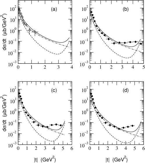
Figure 3: Differential cross sections of model (A) at $E_{\gamma}=$ (a) 2.8, (b) 3.28, (c) 3.55, and (d) 3.82 GeV. The dot-dashed lines are from $\sigma$ exchange and the dashed lines are without $\sigma$ exchange. The solid lines are the full calculation. Experimental data are from Ref. BCGG72 (open squares) and Ref. CLAS01b (filled circles).

The differential cross sections for $\gamma p\to\rho p$ calculated from model (A) are compared with the SLAC data BCGG72 and the recent CLAS data CLAS01b in Fig. 3. We see that the full calculations (solid curves) are dominated by the $\sigma$ exchange contributions (dot-dashed curves). The contributions from the other exchange mechanisms (dashed curves) become comparable only in the very forward and backward angles. This is mainly due to the fact that the Pomeron exchange [Fig. 1(a)] is forward peaked and the $u$-channel nucleon term [Fig. 1(d)] is backward peaked. It is clear that the data can only be qualitatively reproduced by model (A). The main difficulty is in reproducing the data in the large $|t|$ (larger than about 3 GeV²) region. No improvement can be found by varying the cutoff parameters of various form factors of model (A). This implies the role of other production mechanisms in this region.

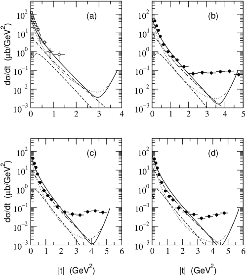
Figure 4: Differential cross sections of model (B) at $E_{\gamma}=$ (a) 2.8, (b) 3.28, (c) 3.55, and (d) 3.82 GeV. The dot-dashed lines are from $f_{2}$ exchange, the dashed lines are from $2\pi$ and $\sigma$ exchanges, and the dotted lines are from the other processes, i.e., without $f_{2}$, $2\pi$, and $\sigma$ exchanges. The solid lines are the full calculation. Experimental data are from Ref. BCGG72 (open squares) and Ref. CLAS01b (filled circles).

The differential cross sections calculated from model (B) are shown in Fig. 4. The solid curves are the best fits to the data we could obtain by choosing the cutoff parameters given in Eq. (51) for the $f_{2}$ exchange. In the same figures, we also show the contributions from the $f_{2}$ exchange (dot-dashed curves), $2\pi$ and $\sigma$ exchanges (dashed curves), and the rest of the production mechanisms (dotted curves). It is interesting to note that the $f_{2}$ exchange in model (B) (dot-dashed curves in Fig. 4) drops faster than the $\sigma$ exchange in model (A) (dot-ashed curves in Fig. 3) as $t$ increases. On the other hand, the $2\pi$ and $\sigma$ exchanges (dashed curves in Fig. 4) give a nontrivial contribution in large $|t|$ region at lower energies but are suppressed as the energy increases. Therefore such effects are expected to be seen at energies very close to the threshold. As expected, the $\sigma$ meson exchange contribution is much suppressed than in model (A).

Thus we find that model (B) is comparable to model (A) that is the commonly used $\sigma$ exchange model in fitting the differential cross section data of SLAC and TJNAF. In particular, the data at small $|t|$ ($<2$ GeV²) can be equally well described by both models, as more clearly shown in Fig. 5, where the full calculations of two models are compared. On the other hand, both models cannot fit the data at large $|t|$ ($>2$ GeV²). But this is expected since we have not included $N^{*}$ and $\Delta^{*}$ excitation mechanisms which were found OTL01 to give significant contributions to $\omega$ photoproduction at large $|t|$. However, we will not address this rather non-trivial issue here. The main difficulty here is that most of the resonance parameters associated with isospin $T=3/2$ $\Delta^{*}$ resonances, which do not contribute to $\omega$ photoproduction, are not determined by Particle Data Group or well-constrained by theoretical models. Before we use our model to determine a large number of resonance parameters by fitting the existing limited data, it would be more desirable to further test and improve the nonresonant amplitudes such as including more complete calculations of $2\pi$-exchanges. Hence, in this paper, we focus on exploring which experimental observables are useful for distinguishing more clearly the Model (B) from Model (A) in the small $|t|$ ($<2$ GeV²) region where both models can describe the differential cross section data to a large extent and the $N^{*}$ and $\Delta^{*}$ effects are expected to be not important. Experimental verifications of our prediction in this limited $t$ region will be useful for understanding the non-resonant amplitudes of $\rho$ photoproduction at low energies.

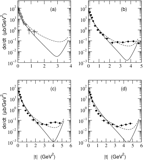
Figure 5: Differential cross sections of model (A) and (B) at $E_{\gamma}=$ (1) 2.8, (b) 3.28, (c) 3.55, and (d) 3.82 GeV. The dashed lines are the results of model (A) and the solid lines are those of model (B). Experimental data are from Refs. CLAS01b ; BCGG72 .

We have explored the consequences of the constructed models (A) and (B) in predicting the spin asymmetries, which are defined, e.g., in Ref. TOYM98 . The results for the single spin asymmetries are shown in Fig. 6 for $E_{\gamma}=3.55$ GeV. Clearly the single spin asymmetries including the target asymmetry $T_{y}$, the recoiled proton asymmetry $P_{y}$, and the tensor asymmetry $V_{xxyy}$ of the produced $\rho$ meson would be useful to distinguish the two models and could be measured at the current experimental facilities. Of course our predictions are valid mainly in the small $t$ region since the $N^{*}$ and $\Delta^{*}$ excitations OTL01 or $G$-pole contributions KV01a-KV02 , which are expected to be important at large $t$, are not included in this calculation.

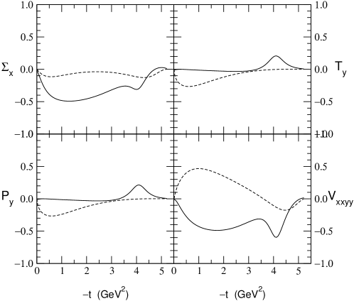
Figure 6: Single spin asymmetries of model (A) and (B) at $E_{\gamma}=3.55$ GeV. Notations are the same as in Fig. 5. The definitions of the spin asymmetries are from Ref. TOYM98 .

Our predictions on the beam-target and beam-recoil double asymmetries TOYM98 are given in Fig. 7. Here again we can find significant differences between the two models in the region of small $|t|$. Experimental tests of our predictions given in Figs. 6 and 7, therefore, will be useful in understanding the non-resonant mechanisms of $\rho$ photoproduction.

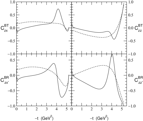
Figure 7: Double spin asymmetries $C^{\rm BT}_{zx}$, $C^{\rm BT}_{zz}$, $C^{\rm BR}_{zx^{\prime}}$, and $C^{\rm BR}_{zz^{\prime}}$ of model (A) and (B) at $E_{\gamma}=3.55$ GeV. Notations are the same as in Fig. 5.

Since both the $\sigma$ and $f_{2}$ exchanges are natural parity exchanges, it would be difficult to test them using parity asymmetry or photon asymmetry that can be measured from the decay distribution of the $\rho$ meson produced by polarized photon beam. For completeness, we give the predictions of the two models on these asymmetries in Fig. 8. As expected, it is very hard to distinguish the two models in the forward scattering angles with these asymmetries.

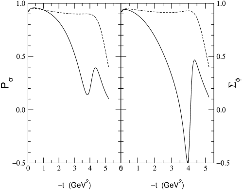
Figure 8: Spin asymmetries $P_{\sigma}$ and $\Sigma_{\phi}$ of model (A) and (B) at $E_{\gamma}=3.55$ GeV. Notations are the same as in Fig. 5.

IV Summary and Discussion

In this paper we have re-examined the $\sigma$-exchange and $f_{2}$-exchange mechanisms of $\rho$ photoproduction reactions. It is found that the commonly employed $\sigma$-exchange amplitude is weakened greatly if the $\sigma$ coupling constants are evaluated by using the recent information about the $\rho\to\pi^{0}\pi^{0}\gamma$ decay and the $\sigma NN$ coupling constant of Bonn potential. This has led us to introduce the un-correlated $2\pi$ exchange amplitude with $\pi N$ intermediate state. This leading-order $2\pi$ exchange amplitude can be calculated realistically using the coupling constants determined from the study of pion photoproduction and the empirical width of $\rho\rightarrow\pi\pi$.

In the investigation of $f_{2}$-exchange mechanism, we evaluate its amplitude using an effective Lagrangian which is constructed from the tensor structure of the $f_{2}$ meson. Phenomenological information together with tensor meson dominance and vector meson dominance assumptions are used to estimate the $f_{2}$ coupling constants. This approach, which is more consistent with the conventional meson-exchange models, is rather different from the $f_{2}$-exchange model of Laget Lage00 , where the $f_{2}$ interaction structure was borrowed from that of Pomeron exchange assuming Pomeron-$f$ proportionality, i.e., $f_{2}$-photon analogy.

In comparing with the existing differential cross section data, we find that a model with the constructed $2\pi$, $\sigma$, and $f_{2}$ exchanges is comparable to the commonly used $\sigma$-exchange model in which the $\sigma$ coupling parameters are simply adjusted to fit data. Both models can describe the data equally well in the small $|t|$ ($<2$ GeV²) region, but fail at large $|t|$. We suggest that experimental verifications of the predicted single and double spin asymmetries in the small $|t|$ region will be useful for distinguishing two models and improving our understanding of the non-resonant amplitude of $\rho$ photoproduction.

Finally, we would like to emphasize that the present investigation is just a very first step toward obtaining a complete dynamical exchange model of $\rho$ photoproduction at low energies. The next steps are to examine the additional $2\pi$-exchange mechanisms due to, for example, $\omega N$ and $\pi\Delta$ intermediate states and the crossed diagrams of Fig. 2. The effects due to $N^{*}$ and $\Delta^{*}$ effects must be included for a realistic understanding of the interplay between the non-resonant and resonant amplitudes. Theoretical predictions of the resonance parameters associated with $\Delta^{*}$ resonance states will be highly desirable for making progress in this direction.

Appendix A Tensor meson dominance and $\bm{f_{2}}$-hadron interactions

The free Lagrangian and the propagator of the tensor meson were studied in Refs. SW63 ; Wei64b ; Chang66 ; BGS94 ; Toub96 . The propagator of the tensor meson which has momentum $p$ reads

$$G^{\mu\nu;\rho\sigma}=\frac{1}{p^{2}-M_{f}^{2}+i\epsilon}P^{\mu\nu;\rho\sigma},$$ (54)

where $M_{f}$ is the tensor meson mass and

$$P^{\mu\nu;\rho\sigma}=\frac{1}{2}\left(\bar{g}^{\mu\rho}\bar{g}^{\nu\sigma}+\bar{g}^{\mu\sigma}\bar{g}^{\nu\rho}\right)-\frac{1}{3}\bar{g}^{\mu\nu}\bar{g}^{\rho\sigma},$$ (55)

with

$$\bar{g}_{\mu\nu}=-g_{\mu\nu}+\frac{p_{\mu}p_{\nu}}{M_{f}^{2}}.$$ (56)

A.1 $\bm{f_{2}\pi\pi}$ coupling

The effective Lagrangian for $f_{2}\pi\pi$ interaction reads PSMM73

$$\mathcal{L}_{f\pi\pi}=-\frac{2G_{f\pi\pi}}{M_{f}}\partial_{\mu}\bm{\pi}\cdot\partial_{\nu}\bm{\pi}f^{\mu\nu},$$ (57)

where $f^{\mu\nu}$ is the $f_{2}$ meson field. This gives the $f_{2}\pi\pi$ vertex function as

$$V_{f\pi\pi}=-\frac{G_{f\pi\pi}}{M_{f}}(p_{a}+p_{c})_{\mu}(p_{a}+p_{c})_{\nu}\epsilon^{\mu\nu}(\lambda_{f}),$$ (58)

where $p_{a}$ and $p_{c}$ are the incoming and outgoing pion momentum, respectively. The minus sign in the Lagrangian (57) is to be consistent with the tensor meson dominance Suzu93 . The Lagrangian (57) gives the $f_{2}\to\pi\pi$ decay width as

$$\Gamma(f_{2}\to\pi\pi)=\frac{G_{f\pi\pi}^{2}}{80\pi}M_{f}\left(1-4\frac{M_{\pi}^{2}}{M_{f}^{2}}\right)^{5/2}.$$ (59)

Using the experimental data, $\Gamma(f_{2}\to\pi\pi)_{\rm expt.}\approx 156.9$ MeV PDG02 , we obtain

$$\frac{G_{f\pi\pi}^{2}}{4\pi}\approx 2.64,$$ (60)

which gives $G_{f\pi\pi}\approx 5.76$.

A.2 Tensor meson dominance

The tensor meson dominance (TMD) is an assumption of meson pole dominance for matrix elements of the energy momentum tensor just as the vector meson dominance (VMD) is a pole dominance of the electromagnetic current. By using TMD, one can determine the universal coupling constant of the $f_{2}$ meson from its decay into two pions, which can then be used to determine the $f_{2}NN$ and $f_{2}VV$ couplings. When combined with VMD, this also allows us to estimate the $f\gamma\gamma$ and $fV\gamma$ vertices. It is interesting to note that the TMD underestimates the empirical $f_{2}NN$ coupling while it overestimates the $f_{2}\to\gamma\gamma$ decay width. But it shows that the $f_{2}$ couplings with hadrons and photon can be understood by TMD and VMD at least qualitatively. Here, for completeness, we briefly review the method of Refs. Renn70 ; Renn71 to illustrate how to use TMD to get the $f_{2}$-hadron couplings.

Let us first apply TMD to spinless particles Renn70 ; Raman71a . The energy-momentum tensor between spinless particles can be written as

$$\langle p|\theta^{\mu\nu}(0)|p^{\prime}\rangle=F_{1}(\Delta^{2})\Sigma_{\mu}\Sigma_{\nu}+F_{2}(\Delta^{2})(\Delta_{\mu}\Delta_{\nu}-g_{\mu\nu}\Delta^{2}),$$ (61)

with $\Sigma_{\mu}=(p+p^{\prime})_{\mu}$ and $\Delta_{\mu}=(p-p^{\prime})_{\mu}$. Then with the covariant normalization one has

$$\langle p|\int\theta_{00}(x)d^{3}x|p\rangle=EN_{p},$$ (62)

where $N_{p}$ is the normalization constant. By comparing with Eq. (61), one can find

$$F_{1}(0)=\frac{1}{2}.$$ (63)

Now we define the effective couplings for tensor mesons as

$$\langle f|\theta_{\mu\nu}(0)|0\rangle=g_{f}M_{f}^{3}\epsilon_{\mu\nu},\qquad\langle p|f|p^{\prime}\rangle=-\epsilon_{\mu\nu}\Sigma^{\mu}\Sigma^{\nu}\frac{G_{fpp}}{M_{f}},$$ (64)

where the latter equation is consistent with Eq. (58). The pole dominance gives

$$\langle p|\theta_{\mu\nu}|p^{\prime}\rangle = \sum_{f}\langle p|f|p^{\prime}\rangle\langle f|\theta_{\mu\nu}|0\rangle\frac{1}{\Delta^{2}-M_{f}^{2}}$$ (65)

$$= -\sum_{f}g_{f}M_{f}^{3}\epsilon_{\mu\nu}\epsilon^{*}_{\alpha\beta}\Sigma^{\alpha}\Sigma^{\beta}\frac{G_{fpp}}{M_{f}}\frac{1}{\Delta^{2}-M_{f}^{2}}$$

$$= -\sum_{f}\frac{g_{f}M_{f}^{2}G_{fpp}}{\Delta^{2}-M_{f}^{2}}\left(\Sigma_{\mu}\Sigma_{\nu}-\frac{1}{3}g_{\mu\nu}\Sigma^{2}+\frac{1}{3}\frac{\Delta_{\mu}\Delta_{\nu}}{M_{f}^{2}}\Sigma^{2}\right),$$

which leads to

$$F_{1}(\Delta^{2})=-\sum_{f}\frac{g_{f}M_{f}^{2}G_{fpp}}{\Delta^{2}-M_{f}^{2}}.$$ (66)

Thus we have

$$F_{1}(0)=\sum_{f}g_{f}G_{fpp}=\frac{1}{2}.$$ (67)

It should be noted that the sum of Eq. (67) contains tensor meson nonet, i.e., $f_{2}(1270)$ and $f_{2}^{\prime}(1525)$. But in the case of the $f_{2}\pi\pi$ coupling, if we assume the ideal mixing between the $f_{2}(1270)$ and the $f_{2}^{\prime}(1525)$, the $f_{2}^{\prime}(1525)$ decouples by the OZI rule. Therefore we obtain $G_{f^{\prime}\pi\pi}\approx 0$, and the universal coupling constant $g_{f}$ is determined as

$$g_{f}=\frac{1}{2G_{f\pi\pi}}\approx 0.087,$$ (68)

using the value of Eq. (60).

With the universal coupling constant $g_{f}$ determined above, one can now use it to estimate the $f_{2}NN$ coupling. For this purpose, we apply TMD to spin-1/2 baryon state. The energy-momentum tensor of the spin-1/2 baryons can be written as

$$\langle p|\theta_{\mu\nu}(0)|p^{\prime}\rangle = \bar{u}(p)\left\{\frac{1}{4}(\gamma_{\mu}\Sigma_{\nu}+\gamma_{\nu}\Sigma_{\mu})F_{1}(\Delta^{2})\right.$$ (69)

$$\mbox{}\left.\qquad\mbox{}+\frac{\Sigma_{\mu}\Sigma_{\nu}}{4M_{N}}F_{2}(\Delta^{2})+(\Delta_{\mu}\Delta_{\nu}-g_{\mu\nu}\Delta^{2})F_{3}(\Delta^{2})\right\}u(p^{\prime}).$$

With the covariant normalization, the conditions

$$\langle p|\int\theta_{00}(x)d^{3}x|p\rangle=EN_{p},$$

$$\langle p,{\bf p}=0,s_{3}=+\textstyle\frac{1}{2}|\int\{x_{1}\theta_{02}(x)-x_{2}\theta_{01}(x)\}d^{3}x|p,{\bf p}=0,s_{3}=+\frac{1}{2}\rangle=\frac{1}{2}N_{p},$$

(70)

give

$$F_{1}(0)=1,\qquad F_{2}(0)=0.$$ (71)

Now using the form for $f_{2}NN$ coupling in Eq. (26), assuming the pole dominance gives the following relations:

$$-1 = 4g_{f}G_{fNN}\frac{M_{f}}{M_{N}}+4g_{f^{\prime}}G_{f^{\prime}NN}\frac{M_{f^{\prime}}}{M_{N}},$$

$$0 = 4g_{f}F_{fNN}\frac{M_{f}}{M_{N}}+4g_{f^{\prime}}F_{f^{\prime}NN}\frac{M_{f^{\prime}}}{M_{N}}.$$ (72)

Again by assuming the decoupling of the $f_{2}^{\prime}$ from the nucleon coupling, we can have Renn70

$$G_{fNN} = \frac{1}{4g_{f}}\frac{M_{p}}{M_{f}}=\frac{G_{f\pi\pi}}{2}\frac{M_{p}}{M_{f}}\approx 2.12,$$

$$F_{fNN} = 0.$$ (73)

This gives $G_{fNN}^{2}/4\pi\approx 0.38$ as shown in Table 1, which is smaller than the values estimated by $\pi N$ dispersion relations by an order of magnitude. It should also be noted that the values estimated by $\pi N$ dispersion relations may be affected by the inclusion of other meson exchanges. More rigorous study in this direction is, therefore, highly desirable.

A.3 $\bm{f_{2}VV}$ coupling

Before we discuss $f_{2}\gamma\gamma$ and $f_{2}V\gamma$ couplings, we first apply TMD to $f_{2}VV$ coupling, where $V$ stands for vector mesons. The energy-momentum tensor between identical vector mesons contains six independent matrix elements Renn71 ,

$$\langle V|\theta_{\mu\nu}|V^{\prime}\rangle = \mathcal{G}_{1}(\Delta^{2})(\epsilon\cdot\epsilon^{\prime})\Sigma_{\mu}\Sigma_{\nu}+\mathcal{G}_{2}(\Delta^{2})(\epsilon\cdot\Sigma)(\epsilon^{\prime}\cdot\Sigma)\Sigma_{\mu}\Sigma_{\nu}$$ (74)

$$\mbox{}+\mathcal{G}_{3}(\Delta^{2})\left\{(\epsilon\cdot\Sigma)\epsilon^{\prime}_{\mu}\Sigma_{\nu}+(\epsilon\cdot\Sigma)\epsilon^{\prime}_{\nu}\Sigma_{\mu}+(\epsilon^{\prime}\cdot\Sigma)\epsilon_{\mu}\Sigma_{\nu}+(\epsilon^{\prime}\cdot\Sigma)\epsilon_{\nu}\Sigma_{\mu}\right\}$$

$$\mbox{}+\mathcal{G}_{4}(\Delta^{2})\left\{(\epsilon\cdot\Delta)\epsilon_{\mu}^{\prime}\Delta_{\nu}+(\epsilon\cdot\Delta)\epsilon_{\nu}^{\prime}\Delta_{\mu}+(\epsilon^{\prime}\cdot\Delta)\epsilon_{\mu}\Delta_{\nu}+(\epsilon^{\prime}\cdot\Delta)\epsilon_{\nu}\Delta_{\mu}\right.$$

$$\mbox{}\qquad\qquad\left.-2(\epsilon\cdot\Delta)(\epsilon^{\prime}\cdot\Delta)g_{\mu\nu}-\Delta^{2}(\epsilon_{\mu}\epsilon_{\nu}^{\prime}+\epsilon_{\mu}^{\prime}\epsilon_{\nu})\right\}$$

$$\mbox{}+\mathcal{G}_{5}(\Delta^{2})(\epsilon\cdot\epsilon^{\prime})(\Delta_{\mu}\Delta_{\nu}-\Delta^{2}g_{\mu\nu})$$

$$\mbox{}+\mathcal{G}_{6}(\Delta^{2})(\epsilon\cdot\Sigma)(\epsilon^{\prime}\cdot\Sigma)(\Delta_{\mu}\Delta_{\nu}-g_{\mu\nu}\Delta^{2}),$$

where $\Sigma_{\mu}=(p+p^{\prime})_{\mu}$, $\Delta_{\mu}=(p-p^{\prime})_{\mu}$ and $\epsilon,\epsilon^{\prime}$ are the polarization vectors of $V$ and $V^{\prime}$, respectively. Then the conditions like Eq. (70) give

$$\mathcal{G}_{1}(0)=-\frac{1}{2},\qquad\mathcal{G}_{3}(0)=\frac{1}{2}.$$ (75)

In the pole model, the form factors $\mathcal{G}_{1}(\Delta^{2})\dots\mathcal{G}_{4}(\Delta^{2})$ are dominated by tensor meson poles. Because of the symmetry property of the tensor meson, we have generally four $f_{2}VV$ coupling vertices:

$$\langle V|f|V^{\prime}\rangle = \frac{G_{1}}{M_{f}}(\epsilon\cdot\epsilon^{\prime})(\Sigma_{\mu}\Sigma_{\nu}f^{\mu\nu})+\frac{G_{2}}{M_{f}^{3}}(\epsilon\cdot\Sigma)(\epsilon^{\prime}\cdot\Sigma)(\Sigma_{\mu}\Sigma_{\nu}f^{\mu\nu})$$ (76)

$$\mbox{}+\frac{G_{3}}{M_{f}}\left\{(\epsilon\cdot\Sigma)\epsilon^{\prime}_{\mu}\Sigma_{\nu}+(\epsilon\cdot\Sigma)\epsilon^{\prime}_{\nu}\Sigma_{\mu}+(\epsilon^{\prime}\cdot\Sigma)\epsilon_{\mu}\Sigma_{\nu}+(\epsilon^{\prime}\cdot\Sigma)\epsilon_{\nu}\Sigma_{\mu}\right\}f^{\mu\nu}$$

$$\mbox{}+\frac{G_{4}}{M_{f}}(-\Delta^{2})(\epsilon_{\mu}\epsilon_{\nu}^{\prime}+\epsilon_{\mu}^{\prime}\epsilon_{\nu})f^{\mu\nu},$$

while we have used $\Delta^{\mu}f_{\mu\nu}=f^{\mu}_{\mu}=0$ in writing the $G_{4}$ term. For our later use, an effective vertex $H(\Delta^{2},p^{2},p^{\prime 2})$ is introduced to replace $-\frac{G_{4}}{M_{f}}\Delta^{2}$ as Renn71

$$H(\Delta^{2},p^{2},p^{\prime 2})=\frac{G_{4}}{M_{f}}\left\{-\Delta^{2}+\alpha(p^{2}+p^{\prime 2}-2M_{V}^{2})\right\}.$$ (77)

Now we use the pole dominance again using Eq. (64) to find

$$\mathcal{G}_{1}(\Delta^{2})=\frac{g_{f}M_{f}^{2}G_{1}}{\Delta^{2}-M_{f}^{2}},$$ (78)

which leads to

$$\frac{1}{2}=g_{f}G_{1},\qquad G_{3}=-G_{1},$$ (79)

combined with Eq. (75). Therefore, with Eq. (68) we get

$$G_{1}=-G_{3}=G_{f\pi\pi}\approx 5.76.$$ (80)

The above relation should hold for $f_{2}\rho\rho$ and $f_{2}\omega\omega$. The SU(3) symmetry and the ideal mixing give

$$G_{1}(f_{2}^{\prime}\phi\phi)=\sqrt{2}G_{1}(f_{2}\rho\rho),\qquad G_{1}(f_{2}^{\prime}\phi\omega)=G_{1}(f_{2}\phi\phi)=0.$$ (81)

Note that two couplings $G_{1}$ and $G_{3}$ are determined by TMD but $G_{2}$ and $G_{4}$ cannot be estimated without further assumptions.

A.4 $\bm{f_{2}\gamma\gamma}$ and $\bm{f_{2}V\gamma}$ couplings

The remaining two couplings $G_{2}$ and $G_{4}$ of Eq. (76) are estimated by using VMD and gauge invariance. We consider $f_{2}\to\gamma\gamma$ using VMD as illustrated in Fig. 9.

Figure 9: $f_{2}\to\gamma\gamma$ decay in vector meson dominance.

By using $\epsilon\cdot k=\epsilon^{\prime}\cdot k^{\prime}=0$ and VMD, we have

$$\langle\gamma(k)\gamma(k^{\prime})|f\rangle = \frac{e^{2}}{(k^{2}-M_{V}^{2})(k^{\prime 2}-M_{V}^{2})}\left\{\frac{\tilde{G}_{1}}{M_{f}}(\epsilon\cdot\epsilon^{\prime})(k-k^{\prime})_{\mu}(k-k^{\prime})_{\nu}f^{\mu\nu}\right.$$ (82)

$$\mbox{}-\frac{\tilde{G}_{2}}{M_{f}^{3}}(\epsilon\cdot k^{\prime})(\epsilon^{\prime}\cdot k)(k-k^{\prime})_{\mu}(k-k^{\prime})_{\nu}f^{\mu\nu}$$

$$\mbox{}+\frac{\tilde{G}_{3}}{M_{f}}\left[-(\epsilon\cdot k^{\prime})\epsilon^{\prime}_{\mu}(k-k^{\prime})_{\nu}-(\epsilon\cdot k^{\prime})\epsilon^{\prime}_{\nu}(k-k^{\prime})_{\mu}\right.$$

$$\left.\mbox{}\qquad\qquad+(\epsilon^{\prime}\cdot k)\epsilon_{\mu}(k-k^{\prime})_{\nu}+(\epsilon^{\prime}\cdot k)\epsilon_{\nu}(k-k^{\prime})_{\mu}\right]f^{\mu\nu}$$

$$\mbox{}\left.+\frac{\tilde{G}_{4}}{M_{f}}[-M_{f}^{2}+\alpha(k^{2}+k^{\prime 2}-2M_{V}^{2})](\epsilon_{\mu}\epsilon_{\nu}^{\prime}+\epsilon_{\mu}^{\prime}\epsilon_{\nu})f^{\mu\nu}\right\},$$

where we have introduced the notation

$$\tilde{G}_{i}=\left(\frac{M_{\rho}^{2}}{f_{\rho}}\right)^{2}G_{i}^{f\rho\rho}+\left(\frac{M_{\omega}^{2}}{f_{\omega}}\right)^{2}G_{i}^{f\omega\omega},$$ (83)

with

$$\langle 0|j_{\mu}^{\rm em}|V\rangle=\frac{M_{V}^{2}}{f_{V}}\epsilon_{\mu}(V).$$ (84)

Because of isospin, there is no mixing between the intermediate $\rho$ and $\omega$ mesons. By looking at the amplitude (82), however, one can find that it is not gauge invariant, i.e., it does not vanish when replacing $\epsilon_{\mu}$ by $k_{\mu}$. This gives a constraint on the couplings. The most general form for $f_{2}\gamma\gamma$ satisfying gauge invariance has two independent couplings as Renn71

$$\langle\gamma(k)\gamma(k^{\prime})|f\rangle = \frac{e^{2}}{M_{V}^{4}}\Bigl{\{}A\left[(\epsilon\cdot\epsilon^{\prime})(k\cdot k^{\prime})-(\epsilon\cdot k^{\prime})(\epsilon^{\prime}\cdot k)\right](k-k^{\prime})_{\mu}(k-k^{\prime})_{\nu}f^{\mu\nu}$$ (85)

$$\mbox{}+B[(\epsilon\cdot\epsilon^{\prime})(k-k^{\prime})_{\mu}(k-k^{\prime})_{\nu}+\epsilon_{\mu}^{\prime}(k-k^{\prime})_{\nu}(\epsilon\cdot k^{\prime})+\epsilon_{\nu}^{\prime}(k-k^{\prime})_{\mu}(\epsilon\cdot k^{\prime})$$

$$\mbox{}\qquad-\epsilon_{\mu}(k-k^{\prime})_{\nu}(\epsilon^{\prime}\cdot k)-\epsilon_{\nu}(k-k^{\prime})_{\mu}(\epsilon^{\prime}\cdot k)$$

$$\mbox{}\qquad-2(k\cdot k^{\prime})(\epsilon_{\mu}\epsilon^{\prime}_{\nu}+\epsilon^{\prime}_{\mu}\epsilon_{\nu})]f^{\mu\nu}\Bigr{\}},$$

which then gives

$$\frac{\tilde{G}_{1}}{M_{f}} = (k\cdot k^{\prime})A+B,$$

$$\frac{\tilde{G}_{2}}{M_{f}^{3}} = A,$$

$$\frac{\tilde{G}_{3}}{M_{f}} = -B,$$

$$\frac{\tilde{G}_{4}}{M_{f}}\left[-M_{f}^{2}+\alpha(k^{2}+k^{\prime 2}-2M_{V}^{2})\right] = -2(k\cdot k^{\prime})B=(k^{2}+k^{\prime 2}-M_{f}^{2})B.$$ (86)

Solving this system at $k^{2}=k^{\prime 2}=0$ and $\tilde{G}_{1}=-\tilde{G}_{3}$ gives

$$A=\tilde{G}_{2}=0.$$ (87)

Since gauge invariance applies to isoscalar and isovector photons separately, we get $G_{2}=0$ for $V=\rho,\omega$. Still we do not fix $\tilde{G}_{4}$ and $\alpha$, but have a constraint,

$$\tilde{G}_{4}(M_{f}^{2}+2\alpha M_{V}^{2})=\tilde{G}_{1}M_{f}^{2}.$$ (88)

To complete the model, let us finally consider $fV\gamma$ vertex. Here again, we use the VMD as in Fig. 10. The gauge invariance of the vertex at $k^{2}=M_{V}^{2}$ and $k^{\prime 2}=0$ leads to

$$\tilde{G}_{4}(M_{f}^{2}+\alpha M_{V}^{2})=\tilde{G}_{1}(M_{f}^{2}-M_{V}^{2}).$$ (89)

Then solving the coupled equations (88) and (89) gives Renn71

$$\tilde{G}_{4}=\tilde{G}_{1}\frac{M_{f}^{2}-2M_{V}^{2}}{M_{f}^{2}},\qquad\alpha=\frac{M_{f}^{2}}{M_{f}^{2}-2M_{V}^{2}}.$$ (90)

Thus we have determined all couplings of Eq. (76) with the relation (83).

Figure 10: $f_{2}\to V\gamma$ decay in vector meson dominance.

The above procedure shows that the $f_{2}\gamma\gamma$ and $f_{2}V\gamma$ vertices can be written with two form factors because of gauge invariance, which read

$$\langle\gamma(k)\gamma(k^{\prime})|f_{2}\rangle = \frac{1}{M_{f}}\epsilon^{\kappa}\epsilon^{\prime\lambda}f^{\mu\nu}A_{\kappa\lambda\mu\nu}^{f\gamma\gamma}(k,k^{\prime}),$$

$$\langle\gamma(k)V(k^{\prime})|f_{2}\rangle = \frac{1}{M_{f}}\epsilon^{\kappa}\epsilon^{\prime\lambda}f^{\mu\nu}A_{\kappa\lambda\mu\nu}^{fV\gamma}(k,k^{\prime}),$$ (91)

where

$$A^{f\gamma\gamma}_{\kappa\lambda\mu\nu}(k,k^{\prime}) = \frac{f_{f\gamma\gamma}}{M_{f}^{3}}\left[g_{\kappa\lambda}(k\cdot k^{\prime})-k^{\prime}_{\kappa}k_{\lambda}\right](k-k^{\prime})_{\mu}(k-k^{\prime})_{\nu}$$ (92)

$$\mbox{}+g_{f\gamma\gamma}[g_{\kappa\lambda}(k-k^{\prime})_{\mu}(k-k^{\prime})_{\nu}+g_{\lambda\mu}k^{\prime}_{\kappa}(k-k^{\prime})_{\nu}+g_{\lambda\nu}k^{\prime}_{\kappa}(k-k^{\prime})_{\mu}$$

$$\mbox{}\qquad\qquad-g_{\kappa\mu}k_{\lambda}(k-k^{\prime})_{\nu}-g_{\kappa\nu}k_{\lambda}(k-k^{\prime})_{\mu}$$

$$\mbox{}\qquad\qquad-2k\cdot k^{\prime}(g_{\kappa\mu}g_{\lambda\nu}+g_{\kappa\nu}g_{\lambda\mu})].$$

The vertex function $A_{\kappa\lambda\mu\nu}^{fV\gamma}(k,k^{\prime})$ can be obtained from $A^{f\gamma\gamma}_{\kappa\lambda\mu\nu}$ by replacing $f_{f\gamma\gamma}$ and $g_{f\gamma\gamma}$ by $g_{fV\gamma}$ and $g_{fV\gamma}$, respectively.

With Eqs. (91) and (92), we can obtain the $f_{2}\to\gamma\gamma$ decay width as

$$\Gamma(f_{2}\to\gamma\gamma)=\frac{M_{f}}{20\pi}\left(\frac{1}{24}f_{f\gamma\gamma}^{2}+g_{f\gamma\gamma}^{2}\right).$$ (93)

Then TMD and VMD give Renn71

$$f_{f\gamma\gamma}=0,\qquad g_{f\gamma\gamma}=e^{2}\left(\frac{1}{f_{\rho}^{2}}+\frac{1}{f_{\omega}^{2}}\right)G_{fVV}.$$ (94)

The vector meson decay constants are $f_{\rho}=5.33$, $f_{\omega}=15.2$, and $f_{\phi}=13.4$. By noting that TMD gives $G_{fVV}=G_{f\pi\pi}$, we get

$$\Gamma(f_{2}\to\gamma\gamma)\approx 8.8\mbox{ keV},$$ (95)

while its experimental value is $\Gamma(f_{2}\to\gamma\gamma)_{\rm expt.}=2.6\pm 0.24$ keV. Thus we can find that this procedure overestimates the experimental value by a factor of $3\sim 4$.

The decay width of $f_{2}\to V\gamma$ can be computed using Eqs. (91) and (92) as

$$\Gamma(f_{2}\to V\gamma) = \frac{M_{f}}{10\pi}(1-x)^{3}\left\{\frac{1}{24}|f_{fV\gamma}|^{2}(1-x)^{4}-(f_{fV\gamma}g^{*}_{fV\gamma}+f^{*}_{fV\gamma}g_{fV\gamma})\frac{x(1-x)^{2}}{12}\right.$$ (96)

$$\mbox{}\left.+|g_{fV\gamma}|^{2}\left(1+\frac{x}{2}+\frac{x^{2}}{6}\right)\right\},$$

where $x=M_{V}^{2}/M_{f}^{2}$. TMD combined with VMD gives Renn71

$$f_{fV\gamma}=0,\qquad g_{fV\gamma}=\frac{e}{f_{V}}G_{fVV}.$$ (97)

This leads to

$$\Gamma(f_{2}\to\rho\gamma)/\Gamma(f_{2}\to\omega\gamma)=\frac{g_{f\rho\gamma}^{2}}{g_{f\omega\gamma}^{2}}=\frac{f_{\omega}^{2}}{f_{\rho}^{2}}=8.14\pm 1.2$$ (98)

and Suzu93

$$\Gamma(f_{2}\to\rho\gamma)/\Gamma(f_{2}\to\gamma\gamma)=2\frac{g_{f\rho\gamma}^{2}}{g_{f\gamma\gamma}^{2}}(1-x)^{3}\left(1+\frac{x}{2}+\frac{x^{2}}{6}\right)=155.$$ (99)

Those quantities are not measured yet. Therefore, measuring those quantities will be very useful to test TMD and VMD.

References

- (1) CLAS Collaboration, E. Anciant et al., Phys. Rev. Lett. 85, 4682 (2000).
- (2) CLAS Collaboration, K. Lukashin et al., Phys. Rev. C 63, 065205 (2001); 64, 059901(E) (2001).
- (3) CLAS Collaboration, M. Battaglieri et al., Phys. Rev. Lett. 87, 172002 (2001).
- (4) CLAS Collaboration, M. Battaglieri et al., Phys. Rev. Lett. 90, 022002 (2003).
- (5) J. Ajaka et al., in Proceedings of 14th International Spin Physics Symposium (SPIN 2000), edited by K. Hatanaka, T. Nakano, K. Imai, and H. Ejiri, AIP Conf. Proc. No. 570 (AIP, Melville, NY, 2001) p. 198.
- (6) T. Nakano, in Proceedings of 14th International Spin Physics Symposium (SPIN 2000), edited by K. Hatanaka, T. Nakano, K. Imai, and H. Ejiri, AIP Conf. Proc. No. 570 (AIP, Melville, NY, 2001) p. 189.
- (7) R. W. Clifft, J. B. Dainton, E. Gabathuler, L. S. Littenberg, R. Marshall, S. E. Rock, J. C. Thompson, D. L. Ward, and G. R. Brookes, Phys. Lett. 64B, 213 (1976).
- (8) T. H. Bauer, R. D. Spital, D. R. Yennie, and F. M. Pipkin, Rev. Mod. Phys. 50, 261 (1978); 51, 407(E) (1979).
- (9) A. I. Titov, T.-S. H. Lee, H. Toki, and O. Streltsova, Phys. Rev. C 60, 035205 (1999).
- (10) J.-M. Laget, Phys. Lett. B 489, 313 (2000).
- (11) Y. Oh and H. C. Bhang, Phys. Rev. C 64, 055207 (2001).
- (12) Y. Oh, Talk at Symposium for the 30th Anniversary of Nuclear Physics Division of the Korean Physical Society, Seoul, Korea, 2002, Jour. Korean Phys. Soc. 43, S20 (2003), nucl-th/0301011.
- (13) S. Capstick and W. Roberts, Prog. Part. Nucl. Phys. 45, S241 (2000).
- (14) Y. Oh, A. I. Titov, and T.-S. H. Lee, Phys. Rev. C 63, 025201 (2001).
- (15) Q. Zhao, Z. Li, and C. Bennhold, Phys. Rev. C 58, 2393 (1998).
- (16) Q. Zhao, Phys. Rev. C 63, 025203 (2001).
- (17) A.I. Titov and T.-S. H. Lee, Phys. Rev. C 67, 065205 (2003).
- (18) Y. Oh and T.-S. H. Lee, Phys. Rev. C 66, 045201 (2002).
- (19) G. Penner and U. Mosel, Phys. Rev. C 66, 055211 (2002).
- (20) B. Friman and M. Soyeur, Nucl. Phys. A600, 477 (1996).
- (21) Y. Oh, A. I. Titov, and T.-S. H. Lee, in NSTAR2000 Workshop: Excited Nucleons and Hadronic Structure, edited by V. D. Burkert, L. Elouadrhiri, J. J. Kelly, and R. C. Minehart, (World Scientific, Singapore, 2000), pp. 255–262, nucl-th/0004055.
- (22) N. I. Kochelev and V. Vento, Phys. Lett. B 515, 375 (2001); 541, 281 (2002).
- (23) R. Machleidt, K. Holinde, and C. Elster, Phys. Rep. 149, 1 (1987).
- (24) A. Bramon, R. Escribano, J. L. Lucio M., and M. Napsuciale, Phys. Lett. B 517, 345 (2001).
- (25) A. Gokalp and O. Yilmaz. Phys. Lett. B 508, 345 (2001).
- (26) SND Collaboration, M. N. Achasov et al., Phys. Lett. B 537, 201 (2002).
- (27) T. Sato and T.-S. H. Lee, Phys. Rev. C 54, 2660 (1996).
- (28) A. Donnachie and P. V. Landshoff, Phys. Lett. B 296, 227 (1992).
- (29) P. G. O. Freund, Phys. Lett. 2, 136 (1962).
- (30) P. G. O. Freund, Nouvo Cimento 5A, 9 (1971).
- (31) R. Carlitz, M. B. Green, and A. Zee, Phys. Rev. Lett. 26, 1515 (1971).
- (32) Yu. N. Kafiev and V. V. Serebryakov, Nucl. Phys. B52, 141 (1973).
- (33) A. Donnachie and P. V. Landshoff, Nucl. Phys. B244, 322 (1984).
- (34) P. V. Landshoff and O. Nachtmann, Z. Phys. C 35, 405 (1987).
- (35) J.-M. Laget and R. Mendez-Galain, Nucl. Phys. A581, 397 (1995).
- (36) M. A. Pichowsky and T.-S. H. Lee, Phys. Rev. D 56, 1644 (1997).
- (37) A. I. Titov, Y. Oh, S. N. Yang, and T. Morii, Phys. Rev. C 58, 2429 (1998).
- (38) A. Gokalp and O. Yilmaz, Phys. Rev. D 64, 034012 (2001).
- (39) T. M. Aliev, A. Özpineci, and M. Savcı, Phys. Rev. D 65, 076004 (2002).
- (40) A. Bramon and R. Escribano, hep-ph/0305043.
- (41) Y. Oh and H. Kim, Phys. Rev. D 68, 094003 (2003).
- (42) Particle Data Group, K. Hagiwara et al., Phys. Rev. D 66, 010001 (2002).
- (43) B. C. Pearce and B. K. Jennings, Nucl. Phys. A528, 655 (1991).
- (44) H. Goldberg, Phys. Rev. 171, 1485 (1968).
- (45) H. Pilkuhn, W. Schmidt, A. D. Martin, C. Michael, F. Steiner, B. R. Martin, M. M. Nagels, and J. J. de Swart, Nucl. Phys. B65, 460 (1973).
- (46) B. Renner, Phys. Lett. 33B, 599 (1970).
- (47) P. Achuthan, H.-G. Schlaile, and F. Steiner, Nucl. Phys. B24, 398 (1970).
- (48) J. Engels, Nucl. Phys. B25, 141 (1970).
- (49) N. Hedegaard-Jensen, Nucl. Phys. B119, 27 (1977).
- (50) E. Borie and F. Kaiser, Nucl. Phys. B126, 173 (1977).
- (51) B. Renner, Nucl. Phys. B30, 634 (1971).
- (52) J. Ballam et al., Phys. Rev. D 5, 545 (1972).
- (53) D. H. Sharp and W. G. Wagner, Phys. Rev. 131, 2226 (1963).
- (54) S. Weinberg, Phys. Rev. 133, B1318 (1964).
- (55) S.-J. Chang, Phys. Rev. 148, 1259 (1966).
- (56) S. Bellucci, J. Gasser, and M. E. Sainio, Nucl. Phys. B423, 80 (1994).
- (57) D. Toublan, Phys. Rev. D 53, 6602 (1996), 57, 4495(E) (1998).
- (58) M. Suzuki, Phys. Rev. D 47, 1043 (1993).
- (59) K. Raman, Phys. Rev. D 3, 2900 (1971).
- (60) H. Terazawa, Phys. Lett. B 246, 503 (1990).