Comparison of Nuclear Suppression Effects on Meson Production at High $p_{T}$ and $p_{L}$

Abstract

The medium effect on the pion distribution at high $p_{T}$ in $AA$ collisions is compared to that of the pion distribution at high $p_{L}$ in $pA$ collisions. Both the suppression of the spectra and the energy losses of the measured pions are studied. Although the medium effect on $p_{T}$ is larger than on $p_{L}$, the difference is found surprisingly to be not as big as one would naively expect.

I Introduction

When partons traverse nuclear medium, whether dense or not, they lose momenta by scattering and gluon radiation. At high transverse momentum $p_{T}$ the effect can be calculated in perturbative QCD, although its reliability is not expected for $p_{T}<10$ GeV/c. At low $p_{T}$, but high longitudinal momentum $p_{L}$, the effect cannot be calculated in pQCD, although it is known that partons suffer momenta losses also in the beam direction. Experimentally, it is the momenta of the produced hadrons that are measured. How they are related to the underlying parton $p_{T}$ and $p_{L}$ distributions is still controversial. But even at the phenomenological level it is unknown what the relationship is between the properties of momentum degradation in the transverse and longitudinal directions. We attempt to shed some light on that relationship in this paper.

There are currently good data on high-$p_{T}\,\pi^{0}$ produced at the Relativistic Heavy-Ion Collider (RHIC) up to $p_{T}=8$ GeV/c at various centralities dd . One can therefore deduce the suppression factor from the $p_{T}$ distributions as a function of $p_{T}$ and centrality. There are no comparable data on the $p_{L}$ distributions from RHIC. At lower energies the data of NA49 at the SPS provide a good description of the effect of baryon stopping in $pA$ collision hf . What we need for comparison with the $p_{T}$ of $\pi^{0}$ is the $p_{L}$ distribution of the produced pions, for which no data are yet available. However, we do have a model calculation of the pion distribution that contains the degradation effect extracted from the observed proton distribution hy ; that will be our input in our study of the suppression factor in the $p_{L}$ distribution.

The two features that we shall compare are very different: the degradation of $p_{T}$ in $Au+Au$ collisions at RHIC and the degradation of $p_{L}$ in $p+Pb$ collisions at SPS. In the absence of any information in the literature on the quantitative or qualitative difference between the two types of degradation effects of the nuclear medium, even a crude estimate of the suppression properties described in a common language would be illuminating. Without a study of the type proposed here, one does not even know whether the strengths of suppression are within the same order of magnitude, especially since the medium in $AA$ collision at RHIC is dense and hot, while the medium in $pA$ collision at SPS is uncompressed and cold.

There is a theoretical issue that is of interest to discuss here. For some time there has been a school of thought that all hadrons are produced by the fragmentations of partons, not only in the transverse direction in the form of jets (which is generally accepted), but also in the longitudinal direction in the form of breaking of strings (as in the dual parton model dpm ). The effect of the nuclear medium has been represented by the modification of the fragmentation function wz in transverse direction, but that of the longitudinal direction is not known. However, fragmentation of partons is not the only way to produce hadrons. Recent investigations have shown that quark recombination can be important in the high $p_{T}$ problem hy2 -fm , in addition to its relevance originally proposed for the high $p_{L}$ problem dh ; hy3 . Since the multiparton distributions needed for recombination are drastically different in the transverse and longitudinal directions, the effect of the nuclear medium is considerably more complicated. In this paper we can avoid dealing directly with those complications by putting the emphasis on the phenomenology of the hadrons produced. For the $p_{T}$ problem we shall use the scaling form of the data hy4 , while for the $p_{L}$ problem the calculated $x_{F}$ distributions that follow from the $pA$ data will be used. Our task is made easier by not deriving the $p_{T}$ and $p_{L}$ distributions, but by focusing on the centrality dependences of those distributions.

Suppression of the meson distribution is like jet quenching at the parton level. In addition to the study of suppression, we shall also consider energy loss, which is another way of quantifying the medium effect. It corresponds to a shift in $p_{T}$ or $p_{L}$ that is necessary for the inclusive cross section in medium to be equivalent to a reference cross section with minimal medium effect. We shall find interesting results in the shift that are very different from the prediction of pQCD. That difference is much larger than the difference between the effects on the transverse and longitudinal motions of the produced mesons.

Since our comparison is between $p_{T}$ in $AA$ collisions and $p_{L}$ in $pA$ collisions, they are two steps removed from each other. When good $p_{L}$ data on identified pions in $AA$ collisions become available, they shall then serve as the intermediate station to make possible two one-step comparisons: (1) between $p_{T}$ and $p_{L}$ in $AA$ collisions, and (2) between $p_{L}$ in $AA$ and $p_{L}$ in $pA$ collisions. What we do here therefore sets the stage for that work to come.

II Suppression of the Pion $p_{T}$ Distribution in $AA$ Collisions

For the $p_{T}$ distribution of pions in nuclear collisions we use the PHENIX data on $\pi^{0}$ production at midrapidity with $p_{T}$ extending to as high as 8 GeV/c dd . A convenient scaling form for that distribution has been found that summarizes the dependence on energy and centrality in terms of a simple analytical formula hy4 ; hy5 . The quantity that we want to study is the suppression factor $S$, which is the ratio of the normalized $p_{T}$ distribution $P$:

$$S(x_{T},N)=P(x_{T},N)/P(x_{T},2)\ ,$$ (1)

where $x_{T}$ is the scaled $p_{T}$ variable

$$x_{T}=p_{T}/K_{0}\ ,$$ (2)

and $N$ is the abbreviated notation for the number of participants $N_{\rm part}$. The scale $K_{0}$ is set at 10 GeV/c for convenience; it is trivial to move it higher when higher $p_{T}$ data become available. If $x^{-1}_{T}dN_{\pi}/dx_{T}$ denotes the $x_{T}$ distribution of produced $\pi^{0}$, averaged over midrapidity and over all azimuthal angle $\phi$, then $P(x_{T},N)$ is defined by

$$P(x_{T},N)={1\over x_{T}}{dN_{\pi}\over dx_{T}}\,\left/\int^{1}_{0}dx_{T}{dN_{\pi}\over dx_{T}}\right.\ .$$ (3)

Instead of determining $P(x_{T},N)$ directly from the data for every $N$ at any given $s$, it is simpler to derive it from the scaling function $\Phi(z)$ that is an excellent fit of all high-energy data for all centralities hy4 ; hy5 . Since the details of the relationship between $P(x_{T},N)$ and $\Phi(z)$ are given in Refs. hy4 ; hy5 , there is no need for us to repeat them here. For the convenience of the reader, they are summarized in the Appendix.

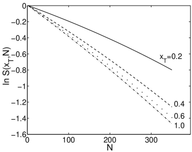
Figure 1: The dependences of the suppression factor $S(x_{T},N)$ on the number of participants $N$ for various values of $x_{T}$.

From the analytical expression for $S(x_{T},N)$ obtained by use of Eq. (60) in Eq. (1) we can examine the $N$ dependence for fixed values of $x_{T}$ by plotting ${\rm ln}S(x_{T},N)$ vs $N$ for some sample values of $x_{T}$, as shown in Fig. 1. Approximating the nearly linear behaviors in Fig. 1 by straight lines, we obtain

$${\rm ln}S(x_{T},N)=a_{0}(x_{T})-a_{1}(x_{T})N\ ,$$ (4)

where $a_{0}(x_{T})$ and $a_{1}(x_{T})$ are shown in Fig. 2. The solid lines in that figure are fits, using the parametrization

$$a_{0}(x_{T})=0.031\left[1-\exp(0.5-12x_{T})\right]\ ,$$ (5)

$$a_{1}(x_{T})=0.0043\left[1-\exp(0.2-5x_{T})\right]\ .$$ (6)

A general statement that can be made about ${\rm ln}S(x_{T},N)$ is that it is approximately linear in $N$, and that the parameters of the linear fits are roughly independent of $x_{T}$ when $x_{T}\geq 0.4$.

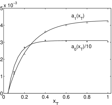
Figure 2: The coefficients $a_{0}(x_{T})$ and $a_{1}(x_{T})$, where $a_{0}(x_{T})$ is plotted with reference to the scale on the left, while $a_{1}(x_{T})$ refers to the scale on the right.

Since the number of participants $N$ is associated only with $AA$ collisions, we must express it in terms of some measure of nuclear length in order to be able to compare the suppression factors in $AA$ and $pA$ collisions. The dependence of $N$ on the impact parameter $b$ is known kn . At a fixed $b$, the lens-shaped overlap region in the transverse plane of two colliding nuclei of the same radius $R_{A}$ has a minimum distance between the center of the overlap and the edge of either nuclei (assumed to have a sharp boundary)

$$L_{\rm min}=R_{A}-b/2\ .$$ (7)

The maximum distance between the center of the overlap to the edge of both nuclei is

$$L_{\rm max}=\left(R^{2}_{A}-b^{2}/4\right)^{1/2}\ .$$ (8)

The distance that a parton would travel in the nuclear medium at midrapidity in the transverse plane can be as large as $2L_{\rm max}$ and as small as 0, depending on where the parton starts and in which direction. We shall set the average distance $L$ traversed to be

$$L(b)=L_{\rm min}=R_{A}-b/2\ ,$$ (9)

which is an approximate average over all azimuthal angles and origins of parton paths. Any more detailed geometrical averaging is pointless, since the nuclear density of the overlap region is not uniform, and the nonuniformity depends on $b$. Knowing $N(b)$ and $L(b)$ enables us to plot $N$ vs $L$, as shown by the solid line in Fig. 3. We shall approximate $N(L)$ by a straight line

$$N(L)=-35.8+62.2L$$ (10)

(with $L$ in units of fm), shown by the dashed line in Fig. 3. In view of the nonuniformity of the nuclear density traversed by a parton in the overlap regions, we believe that an approximation of $N(L)$ by a linear dependence in Eq. (10) is good enough to represent the path length that enters into the description of the momentum degradation effect.

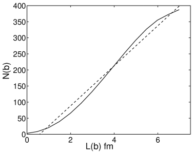
Figure 3: The parametric dependence of $N(b)$ on $L(b)$, where the solid line follows from the use of Eq. (9) for $L(b)$, while the dashed line is a straightline fit of the solid line.

Substituting Eq. (10) into Eq. (4) we obtain

$${\rm ln}S(x_{T},L)=\Lambda_{0}(x_{T})-\Lambda(x_{T})L\ ,$$ (11)

where in $\Lambda_{0}(x_{T})$ the contribution from the $a_{0}(x_{T})$ term in Eq. (4) is negligible. Thus Eq. (11) may be rewritten as

$${\rm ln}S(x_{T},L)=-\Lambda(x_{T})(L-0.71)\ ,$$ (12)

where

$$\Lambda(x_{T})=0.27\left[1-\exp(0.2-5x_{T})\right]\ ,$$ (13)

which is nearly constant for $x_{T}>0.5$, as shown by the solid line in Fig. 4. This exponential dependence of $S(x_{T},L)$ on $L$ is in a familiar form for nuclear attenuation. We remark that although the length $L$ is the approximate average distance in the nuclear medium that a parton traverses, no parton dynamics has been assumed in the derivation of $S(x_{T},L)$, which is extracted from the data on $\pi^{0}$ production without dynamical modeling. The exponential form of $S(x_{T},L)$ is similar to the Gerschel-Hüfner formula for the $J/\psi$ suppression gh , except that the latter refers to a quantity integrated over all $p_{T}$, and is related to the dissociation of $J/\psi$ in the medium. The quarks and antiquarks that form the produced $\pi^{0}$ in our expression for $S(x_{T},L)$ are the results of gluon radiation and gluon conversion processes, most of which are not calculable in pQCD, especially near the end of the evolution process.

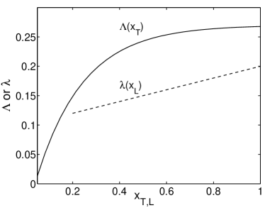
Figure 4: The solid line is for $\Lambda(x_{T})$ and the dashed line is for $\lambda(x_{L})$. The horizontal axis can be for either $x_{T}$ or $x_{L}$.

III Suppression of the Pion $p_{L}$ Distribution in $pA$ Collisions

Since no $p_{L}$ distributions of identified particles in the fragmentation regions of $AA$ collisions at RHIC are available, we consider the processes at the SPS energies. At lower energies the projectile fragmentation region can contain particles arising from the fragmentation of the target, and vice-versa. It is therefore important to consider reactions that are free of such ‘spill-over’ particles. The preliminary data of NA49 on $pA$ collisions at SPS have been analyzed to provide the produced $p-\bar{p}$ distribution of the projectile fragmentation only hf . That is accomplished by determining the $p_{L}$ distribution

$$F_{p}(p-\bar{p})=(p-\bar{p})_{p}-{1\over 2}\left[(p-\bar{p})_{\pi^{+}}+(p-\bar{p})_{\pi^{-}}\right]\ ,$$ (14)

where $(p-\bar{p})_{h}$ denotes the distribution of $h+A\rightarrow(p-\bar{p})+X$, since the quantity inside the square brackets contains no beam fragments by charge conjugation symmetry. A similar distribution for pions, $F_{p}(\pi^{+}-\pi^{-})$, unfortunately does not exist, which is what we need for comparison with the result obtained in the preceding section.

Although there are no experimental data for pion production in the proton fragmentation region free of target fragments, theoretical results on such distributions are available that are based on the centrality dependence of the experimental data of $F_{p}(p-\bar{p})$. In Ref. hy the recombination model is used to relate the data to the nuclear degradation effect on the $p_{L}$ of the produced $p-\bar{p}$, which in turn is then used to predict the $p_{L}$ distributions of the produced pions. Since the nuclear suppression factor on the produced pions is directly related to the experimental suppression of the produced $p-\bar{p}$, we shall use the result in hy for the pion distribution in $p+Pb$ collisions.

Let us use $H(x_{L},\bar{\nu})$ to denote the pion inclusive distribution in the scaled longitudinal momentum, integrated over $p_{T}$, i.e.,

$$H(x_{L},\bar{\nu})=x_{L}{dN_{\pi}\over dx_{L}}\ ,$$ (15)

where $x_{L}=2p_{L}/\sqrt{s}$ and $\bar{\nu}$ is the average number of collisions with nucleons in the target nucleus. From Fig. 9 in Ref. hy one sees that $H(x_{L},\bar{\nu})$ is essentially exponential in $x_{L}$ for various values of $\bar{\nu}$. We use the following parameterization for $p+Pb\rightarrow\pi^{+}+X$

$$H(x_{L},\bar{\nu})=\exp\left[-h_{0}(\bar{\nu})-h_{1}(\bar{\nu})x_{L}\right]\ ,$$ (16)

where

$$h_{0}(3.1)=0.92, h_{0}(6.3)=1.61\ ,$$

$$h_{1}(3.1)=5.89, h_{1}(6.3)=6.57\ .$$ (17)

These parameters provide a good fit for $0.2\leq x_{L}\leq 0.6$. For $x_{L}>0.6$, the slopes are slightly higher, but the ratio of $H(x_{L},\bar{\nu})$ at the two values of $\bar{\nu}$ is about the same.

Since the data are for the two values of $\bar{\nu}$ only, our definition of the suppression factor is

$$S\left(x_{L};\bar{\nu}_{2},\bar{\nu}_{1}\right)=H\left(x_{L},\bar{\nu}_{2}\right)\,\left/H\left(x_{L},\bar{\nu}_{1}\right)\right.$$ (18)

with $\bar{\nu}_{1}=3.1$ and $\bar{\nu}_{2}=6.3$. We now make the assumption that $h_{0}(\bar{\nu})$ and $h_{1}(\bar{\nu})$ are linear functions of $\bar{\nu}$, partly because the average $\langle x_{L}\rangle$ can be shown to decrease exponentially with $\bar{\nu}$ hy , and partly because all nuclear damping effects are empirically dependent on the path length in exponential form. With that assumption we can express $S\left(x_{L};\bar{\nu},1\right)$ for any $\bar{\nu}$ relative to $\bar{\nu}=1$ as

$${\rm ln}S\left(x_{L};\bar{\nu},1\right)=-\left[\theta_{0}(\bar{\nu})+\theta_{1}(\bar{\nu})x_{L}\right]$$ (19)

where $\theta_{0}(\bar{\nu})$ and $\theta_{1}(\bar{\nu})$ are the linear functions of $\bar{\nu}$

$$\theta_{i}(\bar{\nu})=h_{i}(\bar{\nu})-h_{i}(1)=\theta^{\prime}_{i}\,(\bar{\nu}-1)\ ,\qquad i=0,1\ .$$ (20)

The slopes are

$$\theta^{\prime}_{i}={h_{i}(\bar{\nu}_{2})-h_{i}(\bar{\nu}_{1})\over\bar{\nu}_{2}-\bar{\nu}_{1}}\ .$$ (21)

From the values given in Eq. (17), we find that $\theta^{\prime}_{0}$ and $\theta^{\prime}_{1}$ are very nearly equal. We denote them collectively by

$$\theta^{\prime}=0.21$$ (22)

and Eq. (19) becomes

$${\rm ln}S\left(x_{L};\bar{\nu},1\right)=-\theta^{\prime}(1+x_{L})(\bar{\nu}-1)\ .$$ (23)

The exponential dependence of $S$ on $\bar{\nu}$ is now explicit. The specific $x_{L}$ dependence of the decay coefficient is a result of the distribution in Eq. (16) calculated in hy .

If $L$ denotes the path length in a $pA$ collision, then the usual expression for $\bar{\nu}$ in terms of $L$ is

$$\bar{\nu}=\sigma_{pp}\rho L,\qquad\rho={4\pi\over 3}{A\over R^{3}_{A}}\ .$$ (24)

Using $R_{A}=1.2A^{1/3}$ fm, and $\sigma_{pp}=35$ mb, we have

$$\bar{\nu}=0.48L\ ,$$ (25)

where $L$ is in units of fm. Substituting this in Eq. (23) yields

$${\rm ln}S\left(x_{L},L\right)=-\lambda(x_{L})\ (L-2.1)\ ,$$ (26)

where

$$\lambda(x_{L})=0.1\ (1+x_{L})\ .$$ (27)

Equations (26) and (27) for the suppression of the $p_{L}$ distribution in $pA$ collisions are the counterparts of Eqs.  (12) and (13) for the suppression of the $p_{T}$ distribution in $AA$ collisions. Instead of $\Lambda(x_{T})$ that rises rapidly at small $x_{T}$, but saturates to a nearly constant value for $x_{T}>0.5$, as shown in Fig. 4, we now have $\lambda(x_{L})$ which is linearly rising, shown by the dashed line in Fig. 4. Since Eq. (16) is not reliable for $x_{L}<0.2$, we do not show that portion of $\lambda(x_{L})$ in Fig. 4. For numerical comparison we can consider $x_{T}=x_{L}$ at two values, 0.6 and 0.8:

$$\Lambda(0.6)=0.25\ ,\quad\quad\lambda(0.6)=0.16\ ,$$

$$\Lambda(0.8)=0.26\ ,\quad\quad\lambda(0.8)=0.18\ .$$ (28)

Evidently, $\Lambda(x_{T})$ is larger than $\lambda(x_{L})$ when $x_{T}=x_{L}>0.5$, but not by much. Of course, there is no cogent reason to compare them at $x_{T}\approx x_{L}$ since the scale $K_{0}$ in the definition of $x_{T}$ is arbitrary, while $x_{L}$ is Feynman $x_{F}$ and has scaling property. However, with $\Lambda(x_{T})$ being roughly constant for $x_{T}>0.5$, it does not matter what $x_{T}$ is exactly. The relative values of $\Lambda(x_{T})$ and $\lambda(x_{L})$ shown in Eq. (28) give us some indication of how they differ.

IV Energy Losses in $p_{T}$ and $p_{L}$

Another way to quantify the medium effect is in terms of energy loss. Since our aim in this paper is to stay at the level of observable quantities, we cannot descend to the parton level where the concept of energy loss makes sense as one can study the evolution of a parton in its trajectory through the nuclear or quark medium. A produced meson does not itself traverse that medium, since it is only at the end of the evolution of the parton system that it is formed. Nevertheless, the notion of energy loss can be expressed in terms of a shift in $x_{T}$ in comparing the meson inclusive distributions at two different values of $N$. To be specific, let us set the reference value of $N$ at $N=2$, which is not exactly $pp$ collision, but is low enough to represent minimal nuclear effect. Let us then define the shift $X$ in $x_{T}$ by

$$P(x_{T},N)=P(x_{T}+X,2)\ ,$$ (29)

where $P(x_{T},N)$ is the normalized pion distribution defined in Eq. (3). Thus $X$ measures the degradation of the pion $x_{T}$ in changing $N_{\rm part}$ from 2 to $N$.

Using Eq. (60) where $\left<x_{T}\right>$ is calculable by use of Eq. (58), we can solve Eq. (29) and determine $X$ in terms of $x_{T}$ and $N$. At fixed $N$, the dependence of $X$ on $x_{T}$ is nearly perfectly linear. Parametrisizing it as

$$X(x_{T},N)=x_{0}(N)+\xi(N)\ x_{T}\ ,$$ (30)

we find, for $N=100,200,$ and 350, the result $x_{0}(N)=-0.0047,-0.0023,$ and $-0.0039$, and $\xi(N)=0.0432,0.0916,$ and 0.1741, respectively. Since $x_{0}$ is negligible except at very small $x_{T}$, we can regard $\xi(N)$ as the fractional shift, or more precisely as

$$\xi(N)=dX(x_{T},N)/dx_{T}\ ,$$ (31)

whose dependence on $N$ is shown in Fig. 5. Disregarding the point at $N=2$, where by definition $\xi(2)=0$, the three points at $N=100,200,$ and 350 can be fitted by a straight line, as shown by the solid line in Fig. 5. Its parametrization is

$$\xi(N)=-0.011+5.26\times 10^{-4}\ N$$ (32)

for $N\stackrel{{\scriptstyle>}}{{\sim}}50$. Thus for $AA$ collisions the fractional energy loss or fractional shift in $p_{T}$ is independent of $p_{T}$ and depends linearly on $N$ with a coefficient

$$\xi^{\prime}_{N}=5.26\times 10^{-4}\ .$$ (33)

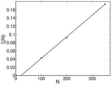
Figure 5: The $N$ dependence of the fractional shift $\xi$. The solid line is a linear fit of the upper three points.

This result can be obtained quickly, but only approximately, in two ways. First, if one ignores the dependence on $N$ of the denominator in Eq. (53), an approximation that amounts to setting $k(s,N)$ to be a constant (an error $\leq 20\%$) compared to the many orders of magnitude of variation of $\Phi(z)$, then the condition of Eq. (29) is equivalent to identifying its two sides with the same function $\Phi(z)$ with $z$ evaluated at $N_{\rm part}=N$ and 2, i.e.,

$$\xi(N) \approx {p_{T}(2)-p_{T}(N)\over p_{T}(N)}={K(2)-K(N)\over K(N)}$$ (34)

$$={6.36\times 10^{-4}\ (N-2)\over K(N)}\ .$$

Setting $K(N)\approx K(2)=1.226$ results in

$$\xi^{\prime}_{N}\approx 5.19\times 10^{-4}\ ,$$ (35)

which is only slightly less than the more accurate value in Eq. (33). The other approximate way of determining the fractional shift is to use Eq. (60) and ignore the $N$ dependence of $\left<x_{T}\right>^{2}$ in that equation so that the condition in Eq. (29) becomes an identification of the $u$ variable in $\Psi(u)$ at two values of $N$, i.e.,

$$u(N)={x_{T}\over\left<x_{T}\right>_{N}}=u(2)={x_{T}+X\over\left<x_{T}\right>_{N=2}}\ .$$ (36)

Since $\left<x_{T}\right>_{N}$ depends on $N$ in a known way hy4

$$\left<x_{T}\right>_{N}=\left<x_{T}\right>_{N_{0}}\ \exp[\,-\beta\,(N-N_{0})]\ ,$$ (37)

where $\beta=5.542\times 10^{-4}$ (denoted by $\lambda$ in hy4 ), its use in Eq. (36) results in

$$\xi^{\prime}_{N}\approx\beta=5.54\times 10^{-4}\ .$$ (38)

Note that the smallness of $\beta$ in Eq. (37) roughly justifies the treatment of $\left<x_{T}\right>$ as a constant in Eq. (60) in the first place. The value of $\xi^{\prime}_{N}$ in Eq. (38) is only slightly larger than that in Eq. (33). Thus the two approximate methods yield results that bracket the correct value closely, and illustrate the crucial role that the scaling variables $z$ and $u$ play.

It is of interest to note that in pQCD the shift in $p_{T}$ of the vacuum spectrum necessary to effect the in-medium spectrum is proportional to $\sqrt{p}_{T}$ bdm . It means that the fractional shift decreases with $p_{T}$, whereas our phenomenological result indicates that it is independent of $p_{T}$. However, since pQCD is reliable only for $p_{T}>10$ Gev/c, while our analysis is based on data at $p_{T}<10$ Gev/c, there is as yet no direct conflict. Nevertheless, the disagreement in the $p_{T}$ dependences is worth bearing in mind.

We now consider the energy loss of $p_{L}$ of pions produced in $pA$ collisions. We define the shift $X$ by referring the inclusive cross section at $\bar{\nu}$ to that at $\bar{\nu}=1$, i.e.,

$$H(x_{L},\bar{\nu})=H(x_{L}+X,1)\ .$$ (39)

The use of Eq. (16) and (20) leads to

$$X(x_{L},\bar{\nu})=\xi(\bar{\nu})\ (x_{L}+1)\ ,$$ (40)

where

$$\xi(\bar{\nu})=\xi^{\prime}_{\bar{\nu}}\ (\bar{\nu}-1)\ ,$$ (41)

$$\xi^{\prime}_{\bar{\nu}}=\theta^{\prime}/h_{1}(1)=0.0385\ .$$ (42)

To compare with the result from $AA$ collisions, let us convert both $N$ and $\bar{\nu}$ to the average path length $L$. Using Eq. (10) in (32), we get

$$\xi_{T}(L)=-0.03+0.0327\ L\ .$$ (43)

Using Eq. (25) in (41), we get

$$\xi_{L}(L)=-0.0385+0.0185\ L\ .$$ (44)

In both cases the fractional shifts depend linearly on $L$ with the coefficients

$$\xi^{\prime}_{T}=0.0327\ ,\qquad\qquad\xi^{\prime}_{L}=0.0185\ .$$ (45)

The ratio of these two coefficients is very nearly the same as the ratio of $\Lambda(x_{T})$ to $\lambda(x_{L})$ in the region $x_{T,L}\approx 0.5$ [cf. Fig. 4]. Thus the study of energy loss and that of suppression give comparable results on the effects of the nuclear medium. The advantage of using Eq. (45) for comparing the nuclear effects on the transverse and longitudinal motions is that the fractional shift is independent of the scale $K_{0}$ used in the definition of $x_{T}$ in Eq. (2). Thus the numerical values of $\xi^{\prime}_{N},\xi^{\prime}_{\bar{\nu}},\xi^{\prime}_{T}$ and $\xi^{\prime}_{L}$ are simple quantitative results of this investigation that can be reexamined in the future when experimental data at different energies for different colliding nuclei become available.

V Conclusion

We have studied the suppression effect of the medium and the energy losses of the produced particles. The former is a comparison of the inclusive distributions in-medium versus minimal-medium at the same $x_{T}$ or $x_{L}$. The latter is the shift in $x_{T}$ or $x_{L}$ necessary for the two distributions at different $N$ to be equivalent. Both studies yield qualitatively the same level of effect. In the following we shall use the suppression effect to represent both in our discussion of the differences between the transverse and longitudinal effects.

The primary remark to make is that the values of $\Lambda(x_{T})$ and $\lambda(x_{L})$ given in Eq. (28) are amazingly close. There are many arguments one can give to suggest that $\Lambda(x_{T})$ and $\lambda(x_{L})$ should not be similar in magnitude, and few are available to explain that they are even within the same order of magnitude. Let us present some of them.

The main difference between the two suppression effects is that one refers to transverse, the other longitudinal motion. For transverse momenta of partons caused by hard collisions, at least there is pQCD to describe some aspects of the dynamics, although not reliably for $p_{T}<8$ GeV/c. For the longitudinal momenta of the particles detected, there is no basic theory to describe their behavior in terms of partons without some substantial use of models. Some properties of the $p_{T}$ degradation can be calculated, but a recent result on the nuclear modification factor does not reproduce even the trend of the $p_{T}$ dependence sw . Nevertheless, much more work has been done in applying pQCD to the high $p_{T}$ problem than to the high $p_{L}$ problem. Since no large momentum transfers are involved at high $p_{L}$, one would naively not expect the nuclear suppression effect to be of the same nature as at high $p_{T}$. Yet we find $\Lambda(x_{T})$ and $\lambda(x_{L})$ to be comparable.

The media of the two problems are also different. In $AA$ collisions at RHIC one expects the nuclear medium to be dense and hot, if not a quark-gluon plasma. In $pA$ collisions at SPS the medium that the projectile traverses is the normal uncompressed nucleus. One would therefore expect the effects of the media on momentum degradation to be very different, yet they are not.

The estimates of the average path length $L$ involve different approximations for the two cases, and it is difficult to assess the effects of those approximations. The only way that $p_{T}$ in $AA$ collisions can be compared to $p_{L}$ in $pA$ collisions is in the common language of exponential decay in terms of a path length $L$. To improve on this problem, we have to gain more information from experiments at intermediate steps by measuring $p_{L}$ in $AB$ collisions with various nuclear sizes of $A$.

We can think of one reason that could possibly explain the closeness of $\Lambda(x_{T})$ to $\lambda(x_{L})$. The inclusive cross sections that we examine for the calculation of the suppression factor $S$ are for pions, not nucleons or other baryons. Whereas leading baryons are strongly related to the valence quarks in the projectile, the pions are more associated with the gluons, which undergo conversion to $q\bar{q}$ pair before hadronization. The depletion of gluons in the nuclear medium can lead to pion suppression in any direction. Evidence for gluon depletion even in $pA$ collisions can be found in the suppression of $J/\psi$ production at large $x_{L}$ jp ; hpp . Our result on the closeness of $\Lambda(x_{T})$ and $\lambda(x_{L})$ may well suggest that gluon depletion is the main mechanism for the suppression of both $p_{T}$ and $p_{L}$ distributions.

In quantitative terms it must be recognized that $\Lambda(x_{T})$ is undisputatively larger than $\lambda(x_{L})$ and therefore provides some comfort that the suppression effect is enhanced when the medium is denser and hotter. What is unexpected is that it is not an order of magnitude larger. In order to fully understand the suppression problem we need a whole set of experiments that measure identified pions at high $p_{T}$ and $p_{L}$ for all combinations of nuclear sizes in $AB$ collisions at high energy. It is important to discover what is universal in the nuclear effects on the produced particles, and what is not. The finding in this paper constitutes an interesting and intriguing beginning in that direction.

Appendix

In this Appendix we summarize the basic formulas that relate $P(x_{T},N)$ to two scaling functions found in hy4 . The first scaling function is

$$\Phi(z)=1200\,(z^{2}+2)^{-4.8}\left(1+25\,{\rm e}^{-4.5z}\right)\ ,$$ (46)

which describes the $p_{T}$ distributions at all $N$ (number of participants) and all $\sqrt{s}$ in terms of one scaling variable

$$z=p_{T}/K(s,N)\ ,$$ (47)

where $K(s,N)=K(s)K(N)$, with hy2 ; hy5

$$K(s)=0.69+1.55\times 10^{-3}\sqrt{s}\ ,$$ (48)

$$K(N)=1.226-6.36\times 10^{-4}N\ ,$$ (49)

$\sqrt{s}$ being in units of GeV and $K(s,N)$ in units of GeV/c. $\Phi(z)$ is related to the $x_{T}$ distribution by

$$\Phi(z)=A(N)k^{2}(s,N){1\over x_{T}}{dN_{\pi}\over dx_{T}}\ ,$$ (50)

where rapidity density is implied, and

$$A(N)=530N_{c}(N)^{-0.9}\ ,\quad N_{c}(N)=0.44N^{1.33}\ ,$$ (51)

and

$$k(s,N)=K(s,N)/K_{0}\ ,$$ (52)

$K_{0}$ being an arbitrary scale, fixed at 10 GeV/c for the definition of $x_{T}$ in Eq. (2). It is a phenomenological fact that the combination of separate factors on the RHS of Eq.  (50) that individually depend on $x_{T}$, $N$ and $s$ results in a universal function that depends explicitly on the one variable $z$ only.

Using Eq. (50) in Eq. (3) yields

$$P(x_{T},N)=\Phi(x_{T},N)\left/\int^{1}_{0}dx_{T}x_{T}\Phi(x_{T},N)\right.$$ (53)

where $\Phi(z)$ is expressed in terms of $x_{T}$ and $N$ through

$$z=x_{T}/k(s,N)\ .$$ (54)

Dependences of $P$ and $\Phi$ on $s$ will not be shown explicitly. With Eq. (53), the distribution $P(x_{T},N)$ can thus be analytically calculated. However, instead of performing the integration in the denominator for every $N$, there is an even simpler relationship that makes use of another scaling function.

It is found in Ref. hy4 that there exists another scaling function

$$\Psi(u)=\Phi(z(u))\,\left/\int du\,u\,\Phi(z(u))\right.,$$ (55)

where

$$u={p_{T}\over\left<p_{T}\right>}={x_{T}\over\langle x_{T}\rangle}={z\over\langle z\rangle}\ .$$ (56)

The new scaling variable $u$ endows $\Psi(u)$ with a property that is analogous to the Koba-Nielsen-Olesen (KNO) scaling kno . The average $\langle z\rangle$, defined by

$$\langle z\rangle={\int dzz^{2}\Phi(z)\over\int dzz\Phi(z)}\ ,$$ (57)

is a constant $\left<z\right>=0.414$, and is related to $\left<x_{T}\right>$ by

$$\langle z\rangle=\langle x_{T}\rangle/k(s,N)$$ (58)

due to Eq. (54), where $\langle x_{T}\rangle$ is defined by

$$\langle x_{T}\rangle=\int dx_{T}x_{T}{dN_{\pi}\over dx_{T}}\left/\int dx_{T}{dN_{\pi}\over dx_{T}}\right.\ .$$ (59)

A comparison between Eqs. (53) and (55) yields

$$\Psi(u)=\langle x_{T}\rangle^{2}P(x_{T},N)\ .$$ (60)

It is the combination of Eqs. (56) and (60) that has led us to regard $\Psi(u)$ as a KNO-type scaling. The advantage of dealing with $u$ instead of $z$ is that $k(s,N)$ is not explicitly involved in relating $u$ to the observable $p_{T}$. Evaluating Eq. (55), we have hy4

$$\Psi(u)=2.1\times 10^{4}\,(u^{2}+11.65)^{-4.8}\left(1+25e^{-1.864u}\right).$$ (61)

Using Eqs. (58) and (60), we now have an algebraic formula for $P(x_{T},N)$, which can be used directly in Eq. (1) for the suppression factor $S(x_{T},N)$.

References

- (1) D. d’Enterria (PHENIX Collaboration), hep-ex/0209051, talk given at Quark Matter 2002, Nantes, France (2002).
- (2) H. G. Fischer, (NA49 Collaboration), talk given at Quark Matter 2002, Nantes, France (2002), nucl-ex/0209043; B. Cole, talk given at Quark Matter 2001, Stony Brook, NY, (unpublished).
- (3) R. C. Hwa, and C. B. Yang, Phys. Rev. C 65, 034905 (2002).
- (4) A. Capella, U. Sukhatme, C.-I. Tan and J. Tran Thanh Van, Phys. Report 236, 225 (1994).
- (5) X. N. Wang and Z. Huang, Phys. Rev. C 55, 3047 (1997).
- (6) R. C. Hwa, and C. B. Yang, Phys. Rev. C 67, 034902 (2003).
- (7) V. Greco, C. M. Ko and P., Lévai, nucl-th/0301093.
- (8) R. J. Fries, B. Müller, C. Nonaka and S. A. Bass, nucl-th/0301087.
- (9) K. P. Das and R. C. Hwa, Phys. Lett. 68B, 459 (1977); R. C. Hwa, Phys. Rev. D22, 1593 (1980).
- (10) R. C. Hwa, and C. B. Yang, Phys. Rev. C 66, 025205 (2002).
- (11) R. C. Hwa, and C. B. Yang, Phys. Rev. Lett. (to be published), nucl-th/0301004.
- (12) R. C. Hwa, and C. B. Yang, Phys. Rev. C (to be published), nucl-th/0302006.
- (13) D. Kharzeev and M. Nardi, Phys. Lett. B 507, 121 (2001).
- (14) C. Gerschel and J. Hüfner, Phys. Lett. B 207, 253 (1988); Z. Phys. C 56, 171 (1992).
- (15) R. Baier, Yu. Dokshitzer, A. Mueller, and D. Schiff, J. High Energy Physics 0109, 033 (2001).
- (16) C. A. Salgado and U. A. Wiedemann, hep-ph/0302184.
- (17) M. J. Leitch et. al., FNAL E866/NuSea Collaboration, Phys. Rev. Lett. 84, 3256 (2000).
- (18) R. C. Hwa, J. Pišút, and N. Pišútová, Phys. Rev. Lett. 85, 4008 (2000); Phys. Rev. C 64, 054611 (2001).
- (19) Z. Koba, H. B. Nielsen, and P. Olesen, Nucl. Phys. B40, 317 (1972).