Kinematical classification of two-pion production on the nucleon

Abstract

We give a full kinematical classification of all the tree-level two-pion photoproduction processes on the nucleon, which consists of seventeen diagrams. It suggests a method of analysis of two-pion data with little model bias.

I Introduction

Theoretically, photo- and electroproduction of two pions on the nucleon is notoriously difficult due to the complexity and numerous processes involved. A serious attempt would require close to a hunderd distinct diagrams. Model assumptions often appear in the data analysis by the restricted choice of processes. Therefore it is necessary to make a systematic study, and catagorizes these processes. This paper has the limited goal of classifying all the processes by their kinematical properties and showing their characteristics, similar to the $s$-, $t$-, and $u$-channel distinction of 2-to-2 scattering.

The two-pion production on the nucleon plays a pivotal role in the analysis of baryon resonances in the intermediate energies as it is the dominant final state. However, the analysis is often restricted. Most of the time the analysis is performed on integrated quantities, where only a subset or a projection of the five-dimensional data is used. Experiments with almost $4\pi$ acceptance would still have problems to fill the last gaps at forward angles, where certain $t$-channel processes are important. Furthermore, the analysis is often of the type of an isobar model, which focuses on $s$-channel processes.

In the two-pion data the contact, or Kroll-Ruderman, term plays a dominant part. It is the contact photo-production of a pion on the nucleon, and has the structure given by the $\pi NN$ coupling where the derivative in the interaction $i\partial^{\mu}$ is replaced by the minimal photon coupling $eA^{\mu}$. The nucleon can be left in the excited state. For example, Murphy and Laget Murphy:1996ms included $\Delta$ and $N^{\ast}$ excitations for the nucleon, which decayed under the emission of a second pion.

The width of a resonance can only be reproduced by an infinite summation of a perturbative series. From this and the strength of the interaction it can be argued that a perturbative approach has a limited applicability, especially once the energy is larger, such as for the second resonance region around 1.6 GeV. However, Gómez Tejedor and Oset GomezTejedor:1995pe did pursue chiral perturbation theory to analyse different isospin channels up to this energy. They were able to trace certain channels back to particular baryon resonances. A similar, but more limited analysis was performed by Ochi, Hirata, and Takaki. Ochi:1997ev ; Hirata:gr The Valencia group also restricted itself to particular subprocesses and the structure of the $N(1520)$ resonance GomezTejedor:1995kj and the $\Delta(1700)$ resonanceNacher:2000eq as seen in the two-pion production.

Although polarization is important to distinguish different angular momentum states, and in, for example, the Gerasimov-Drell-Hearn sum rule Nacher:2001yr , the polarized large acceptance data is not common. Hence at the moment it seems more important to focus on kinematical separation of the different production processes, which we do in this short paper.

Figure 1: The seventeen tree-level production processes labeled by their intermediate states. The solid lines are all possible baryons, the double lines all possible mesons, and the dashed lines are pions.

II Theory

If one lumps all the baryon and baryonic excitations together, and do the same with all the mesonic states one is still left with seventeen possible production tree diagrams, which are shown in Fig. 1. We ignored the Vector Meson Dominance diagrams where the photon oscillates to a rho-meson, which we consider a vertex function, or form factor. These diagrams, apart from the possible vertex functions we will discuss later, depend only on a restricted set of invariant momenta, which are indicated by the letters in the figure. If we denote the incoming nucleon four-momentum by $p_{ni}$, the outgoing nucleon momentum by $p_{nf}$, and the two pion momenta by $p_{\pi 1}$ and $p_{\pi 2}$, we have the following set of functions of a single momentum squared:

$$s{\rm-channel\ production} : S(p_{nf}+p_{\pi 1}+p_{\pi 2})\ \ ,$$ (1)

$$t{\rm-channel\ production} : T(p_{nf}-p_{ni})\ \ ,$$ (2)

$$u{\rm-channel\ production} : U_{\alpha}(p_{ni}-p_{\pi\alpha})\ \ ,$$ (3)

$${\rm cascade;\ decay\ product} : C_{\alpha}(p_{nf}+p_{\pi\alpha})\ \ ,$$ (4)

$$\pi-\pi{\rm-channel} : R(p_{\pi 1}+p_{\pi 2})\ \ ,$$ (5)

$$\pi{\rm-photon\ interaction} : P_{\alpha}(p_{nf}+p_{\pi\alpha}-p_{ni})\ \ ,$$ (6)

$${\rm late\ photon\ absorption} : X(p_{ni}-p_{\pi 1}-p_{\pi 2})\ \ .$$ (7)

If the pions are identical one should sum $p_{\pi 1}\leftrightarrow p_{\pi 2}$, otherwise there are two functions $\alpha=1,2$ for $U_{\alpha}$, $C_{\alpha}$, and $P_{\alpha}$. Excluding final-state interactions, the amplitude is the particular linear combination of the functions of these variables, shown in Fig. 1. Furthermore, the functions $S,U,X,$ and $C$ can only contain the baryonic resonances, while the functions $P,R,$ and $T$ only the mesonic resonances. As they stand, the kinematical diagrams, which contain only the denominator of the propagators, indicated by a single letter have the dimension of $[{\rm energy}]^{-2}$ and the double letter diagrams $[{\rm energy}]^{-4}$, together with vertex functions and dimensionful coupling constants they should yield a dimensionless invariant amplitude.

Of course, a careful spin, isospin, and partial wave analysis will exclude particular combinations for spin-isospin quantum numbers of the final state. For example, the neutral pion will not generate photo-pion interactions, hence, that amplitude will not depend on $P$. However, at the moment we are more interested to determine the kinematical signatures of each of the processes. It has been the custom to ignore the $t$- and $u$- processes, however, at the typical scattering energies nowadays where pions are fully relativistic, there is no a priori reason to do so.

It is difficult to represent five-dimensional differential cross sections. For two-pion data one often plots the Dalitz plot, which is the density of events for a given invariant mass $m^{2}_{n1}=(p_{nf}+p_{\pi 1})^{2}$ and $m^{2}_{n2}=(p_{nf}+p_{\pi 2})^{2}$. These two variables determine the length of each of the 3-momentum $|{\bf p}_{nf}|$, $|{\bf p}_{\pi 1}|$, and $|{\bf p}_{\pi 2}|$, in a given frame. However, their orientation with respect to the initial scattering direction ${\bf p}_{\gamma}$ is not fixed. For unpolarized scattering there are two angles, which give the rigid-body rotation of the triangle ${\bf p}_{nf}-{\bf p}_{\pi 1}-{\bf p}_{\pi 2}$ in the center-of-mass frame with respect to the vector ${\bf p}_{\gamma}$, while for a polarized photon there is an additional angle with respect to the polarization direction ${\bf e}_{\gamma}$. For unpolarized production processes in the $s$-channel ($S$), the amplitude is constant for these angles. For all the others there is an angular dependence, which might be weak.

The propagators are taken to be polarization averaged. If all the spin projections of a state are summed, it yields a projection on the relative momenta $k_{1}-k_{2}$ of the decay products orthogonal to the momentum $p$ of the decaying particle. Hence

$$\Gamma^{(l)}(p,k_{1},k_{2})=\langle p^{0},{\bf p}|k^{0}_{1},{\bf k}_{1};k^{0}_{2},{\bf k}_{2}\rangle=\left(((k_{2}-k_{1})\cdot p)^{2}-p^{2}(k_{2}-k_{1})^{2}\right)^{l/2}\ \ .$$ (8)

Figure 2: The two kinematical cases studied here, given in the center-of-mass frame. Parallel kinematics ($\parallel$) means the incoming and outgoing nucleon have their momentum in the same direction. Perpendicular kinematics means that the incoming nucleon momentum is perpendicular to both the outgoing nucleon and pion momenta.

The general effect of such a vertex factor is a suppression at threshold of the decay product. It is not difficult to insert factors like these in the invariant amplitudes, however, since we are interested in a general classification only, we use unit vertex functions everywhere. For each channel we insert a single resonance:

$$S(p^{2}) = \frac{1}{p^{2}-M_{s}^{2}+i\Gamma_{s}}\ \ ,$$ (9)

$$C(p^{2})=U(p^{2})=X(p^{2}) = \frac{1}{p^{2}-M_{c}^{2}+i\Gamma_{c}}\ \ ,$$ (10)

$$T(p^{2})=R(p^{2}) = \frac{1}{p^{2}-m_{r}^{2}+i\Gamma_{r}}\ \ ,$$ (11)

$$P(p^{2}) = \frac{1}{p^{2}-m_{\pi}^{2}+i\epsilon}\ \ ,$$ (12)

where we have taken the general idea of a second, or higher resonance in the $s$-channel, a lower resonance in the $c$, $x$, and $u$-channel, and a meson resonance in the $t$ and $r$ channel. The pion is taken as an elementary particle in the photon interaction. The invariant amplitude corresponds to the complex multiplication of the corresponding functions. To investigate the angular dependence, we study two cases: the incoming nucleon parallel to the outgoing nucleon ($\parallel$), and the incoming nucleon perpendicular to the outgoing momenta in the center-of-mass frame ($\perp$). (See Fig. 2.) This does not exhaust the angular dependence, but will give a good indication for each of the processes.

III Results

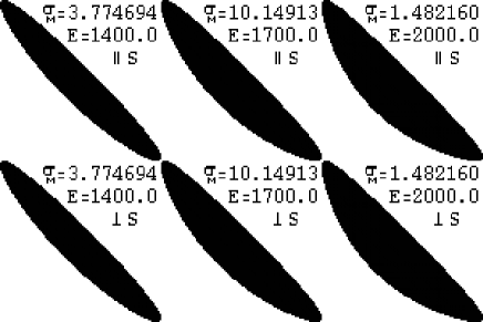
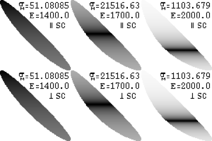
Figure 3: The Dalitz plots for the $S$ and $SC$ processes, the top number is the maximum value of the invariant amplitude squared, the next number is the energy in the center-of-mass frame, $\sqrt{s}$, and $\parallel$ or $\perp$ indicate the direction of the incoming nucleon momenta with respect to the outgoing nucleon momenta

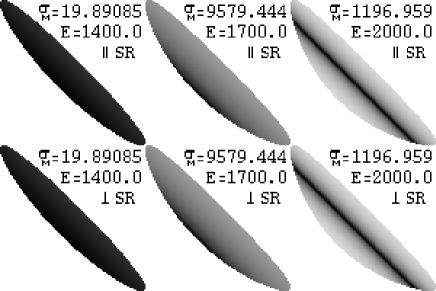
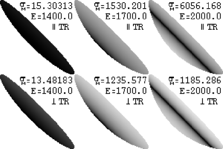
Figure 4: The Dalitz plots for the $SR$ and $TR$ processes.

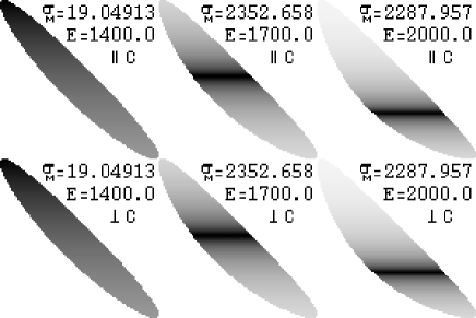
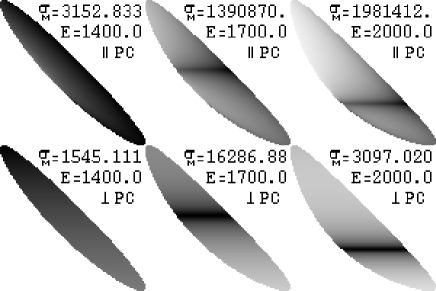
Figure 5: The Dalitz plots for the $C$ and $PC$ processes.

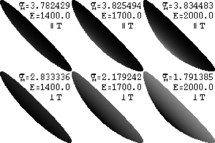
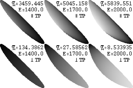
Figure 6: The Dalitz plots for the $T$ and $TP$ processes.

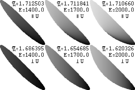
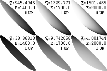
Figure 7: The Dalitz plots for the $U$ and $UP$ processes.

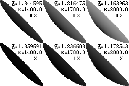
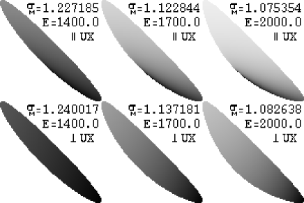
Figure 8: The Dalitz plots for the $X$ and $UX$ processes.

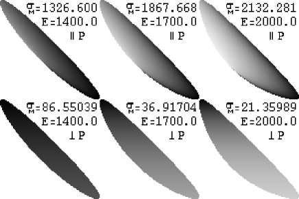
Figure 9: The Dalitz plots for the $P$ and $C$ processes.

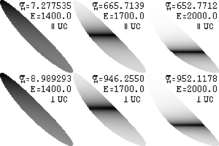
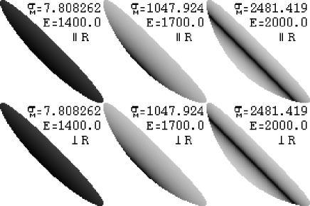
Figure 10: The Dalitz plots for the $UC$ and $R$ processes.

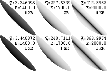
Figure 11: The Dalitz plots for the $XR$ process.

We calculated the invariant amplitude squared $\sigma_{M}$ on a $100\times 100$ grid for each of the seventeen diagrams for the two angular cases and three values of the invariant mass $E=\sqrt{s}$. The values we inserted are not necessarily realistic, but archetypical: $M_{s}=1.6$GeV, $M_{c}=1.35$GeV, $m_{r}=0.77$GeV, and $m_{\pi}=0.14$GeV. The widths are all set to $\sqrt{\Gamma}=0.14$GeV, except the pion which has a small width of $\sqrt{\epsilon}=0.003$GeV. It takes about five seconds to calculate these 102 Dalitz plots independently on a normal desktop computer, which makes a fitting procedure in this approach feasible. The results are shown in Figs. 3-11, the trivial case of “1” is not given.

The $S$ process gives a flat invariant amplitude across the Dalitz plot. The $s$-resonance can be recovered from comparing different scattering energies. All the $S\ast$ processes have no angular dependence as expected, so do the $R$ and $C$ processes. Vertex functions will introduce angular dependence in the latter cases. The $U$ and $X$ processes have signatures that depend on the angle, however, they are not particularly peaked for parallel kinematics. Unlike the $P$ process, which is largely in the forward direction, where the intermediate pion momentum is close to shell, which is also the reason for the large values for this amplitude. The $T$ process is somewhere in between: it has a larger amplitude in parallel kinematics. Only the $S$, the $C$, and the $R$ processes give a clear resonance structure. It is clear why many theoretical studies focus on these diagrams, including combinations like $SC$, and $SR$. However, from this kinematical study it is clear that none of the other processes is obviously suppressed. One of the most complete studies by Murphy and Laget Murphy:1996ms included the diagrams: $C_{\Delta},$ $C_{N^{\ast}},$ $(U_{\Delta}C_{\Delta}),$ $(S_{p}C_{\Delta}),$ $(S_{D_{13}}C_{\Delta}),$ $(S_{P_{11}}C_{\Delta}),$ $(S_{D_{13}}R_{\rho}),$ $(S_{P_{11}}R_{\sigma}),$ $(PC_{\Delta}),$ $(PC_{N^{\ast}}),$ $R_{\rho},$ and $(T_{\rm Pomeron}R_{\rho})$, which is clearly still a small subset of all diagrams. In some two-body baryon resonance analysis effective two-pion states are included, labeled by their angular momentum $\sigma(S=0)$ or $\rho(S=1)$. It would be appropriate to check these channels against the data. However, even from this small kinematical study it is clear that this is not a trivial task.

Furthermore, assuming that $SC$ and $C$ and the dominant parts of the amplitude, we explored possible non-trivial interference in the amplitude. However, in the case of just the single product of two production amplitudes nothing unexpected happens; the interference is more or less the product of the two amplitudes.

IV Conclusions

For the analysis of the data the complexity is significantly reduced if the data is fitted only with arbitrary functions $S,T,U,C,X,R,P$, possibly separated in partial waves for $S$ and $C$. However, it is clear that partial wave analysis might have to yield to combined analysis in problems like these. To first order, the functions are sums of simple single channel resonances, which masses and widths should be recovered, taking care of all the interference among the different parts. The angular information turned out to be important to separate the large non-resonant background from the closed channels.

However, the widths are the direct result of the coupling of a particular resonance to its decay channels. In a proper analysis the coupling strengths and the widths are highly correlated. Therefore, in order to recover this consistency one has to go beyond the perturbation theory described in this paper and typically applied to this problem, and include final-state and intermediate-state interactions in the analysis. This analysis is under investigation. The results presented in this paper, of all the possible production processes, are a first step in this analysis.

References

- (1) L. Y. Murphy and J. M. Laget, DAPNIA-SPHN-96-10
- (2) J. A. Gomez Tejedor and E. Oset, Nucl. Phys. A 600, 413 (1996).
- (3) M. Hirata, K. Ochi and T. Takaki, Prog. Theor. Phys. 100, 681 (1998).
- (4) K. Ochi, M. Hirata and T. Takaki, Phys. Rev. C 56, 1472 (1997).
- (5) J. A. Gomez Tejedor, F. Cano and E. Oset, Phys. Lett. B 379, 39 (1996).
- (6) J. C. Nacher, E. Oset, M. J. Vicente and L. Roca, Nucl. Phys. A 695, 295 (2001).
- (7) J. C. Nacher and E. Oset, Nucl. Phys. A 697, 372 (2002).