Towards a practical approach for self-consistent large amplitude collective motion

Abstract

We investigate the use of an operatorial basis in a self-consistent theory of large amplitude collective motion. For the example of the pairing-plus-quadrupole model, which has been studied previously at equilibrium, we show that a small set of carefully chosen state-dependent basis operators is sufficient to approximate the exact solution of the problem accurately. This approximation is used to study the interplay of quadrupole and pairing degrees of freedom along the collective path for realistic examples. We show how this leads to a viable calculational scheme for studying nuclear structure, and discuss the surprising role of pairing collapse.

I Introduction

There is a general quest for understanding of complicated phenomena in terms of a limited set of degrees of freedom, chosen through some method appropriate for the problem at hand. Many approaches are available, in areas ranging from field theories to atomic physics (see, e.g., the reviews in Ref. To98 ). These are typically based on the concept of “relevant degrees of freedom”, or on the introduction of collective motion and collective paths – which are two ways to express rather similar principles!

More specific to the nuclear problem studied in this paper, the old question “what is the correct choice of collective coordinate in a many-body system” has had quite a few partial answers, see the review DK00 for a discussion of some of these. The holy grail of this approach is a method that determines a collective path self-consistently, based only on knowledge of the Hamiltonian governing the system. Preferably the method chosen should allow us to measure whether the limited dynamics in a few coordinates makes sense at all, or in the language used above, address the question “how effective are the effective degrees of freedom?”.

The constrained Hartree-Fock-Bogoliubov method is commonly used to describe collective paths in nuclear physics (see e.g. BK67 ; RS80 ). This approach, where the collective subspace is generated by a small number of one-body constraints, also goes by the name of generalised cranking. The one-body constraints usually consist of a few carefully chosen multipole (particle-hole) operators, as well as a few generalised pairing (particle-particle) ones. For large scale realistic problems such as the description of nuclear fission the number of generalised cranking operators needed in order to make a realistic calculation becomes very large. There is also no reason to limit the constraints to the standard choices; other degrees of freedom, especially those involving spin-orbit interactions might also be important. A more satisfactory method should allow the cranking operators to be determined by the nuclear collective dynamics itself.

One such approach, followed in this paper and set out in detail in the review paper DK00 (a similar approach, plus relevant references, can be found in Ref. KN03 ), leads to a very well-defined approach, which can in principle be solved knowing the Hamiltonian and model space. To find the adiabatic collective path we use the local harmonic approximation (LHA). It consists of a constrained mean-field problem that needs to be solved together with a local random phase approximation (RPA), which determines the constraining operator. This approach lacks practicality, since the size of the RPA problem is, for a system with pairing, proportional to the size of the single-particle space squared. Even though enormous matrices can routinely be diagonalised on modern computer systems, the algorithm requires repeated diagonalisation of such a matrix, which makes an implementation in realistic calculations prohibitively time consuming.

This requires a solution, or at least a good approximation, and this is the subject of the present paper. A first approach to solving the problem has been suggested in the work of one of the authors NW99 . The best way to test such ideas is to use a semi-realistic model, where approximations can be tested against the full method, such as the pairing-plus-quadrupole model as employed by Barranger and Kumar BK68 in their seminal work. It has been shown in the past NW99 that at equilibrium the RPA can be solved quite efficiently using a simple basis of operators. Related work by Nesterenko et al. NK02 may also have some bearing on this problem, but will not be investigated here. In short, the idea is that the basic operators of the model, weighted by a suitable power of the quasi-particle energies, give excellent results. The state dependence induced by the quasi-particle energies is crucial to the success of the approach, and is the main difference with methods based on “naive” constraints. Since the original work was only done at equilibrium, we must still check that such a basis of operators provides a good solution along the collective path, and we indeed find some important modifications to the method discussed in NW99 . Once a collective path has been found we can diagonalise the collective one-body Hamiltonian along this path, including all the zero modes arising from broken symmetries. This will give information on how the collective motion influences the ground state properties of the nuclei. In several of the examples discussed below we find low lying states with pairing collapse which influence the collective behaviour of the system. If we now quantise the collective dynamics, we must include the pairing rotations. This is due to the fact that a point with collapsed pairing behaves similarly to the origin in polar coordinates, with the pairing phase playing the role of the polar angle. In this work we shall only study the effect of the pairing-rotational modes, ignoring collective rotation for the time being.

The paper is organised as follows. In Sec. II we briefly present the basic principles of our approach, to highlight those issues that will make the results easier to understand. The practical form of the equations for the type of many-body problem considered here is also discussed, and the form of the approximation is introduced. Results are then given in Sec. III and finally we draw some conclusions in Sec. IV.

II Formalism

The formalism, as set out in detail in DK00 , is based on time-dependent mean field theory, and the fact that a classical dynamics can be associated with it. The issue of selecting collective coordinates, and determining their coupling to other degrees of freedom, thus becomes an exercise in classical mechanics. Furthermore, if we assume adiabaticity, a slow motion where the Hamiltonian can be expanded to second order in momenta, we have a problem that can be solved. The solution can be stated without any direct reference to the original nuclear many-body problem and the choice of the interaction.

II.1 Local harmonic approximation for the collective path in the adiabatic limit

We assume a classical Hamiltonian depending on a set of real canonical coordinates, $\xi^{\alpha}$ ($\alpha=1,\ldots,N$), and conjugate momenta, $\pi_{\beta}$ ($\beta=1,\ldots,N$), of the form ($\xi$ and $\pi$ thus parametrise $\left|\Psi\right>$ DK00 )

$${\cal H}(\xi,\pi)=\left<\Psi\right|H\left|\Psi\right>.$$ (1)

We shall use a tensor notation, where we use upper indices for coordinates and lower indices for momenta. When the same symbol appears as both upper and lower index there is an implicit sum over that index.

The potential $V(\xi)={\cal H}(\pi=0)$ and the mass matrix $B^{\alpha\beta}$ are given by an expansion of ${\cal H}(\xi,\pi)$ in powers of $\pi$ in zeroth and second order, respectively,

$${\cal H}(\xi,\pi)=V(\xi)+\frac{1}{2}B^{\alpha\beta}\pi_{\alpha}\pi_{\beta}+{\cal O}(\pi^{4}).$$ (2)

Terms of higher order (such as $\pi^{4}$) are supposed to be negligible. The kinetic energy in the Lagrangian formalism contains the inverse $B_{\alpha\beta}$ of the mass matrix, $K=\frac{1}{2}\dot{\xi}^{\alpha}B_{\alpha\beta}\dot{\xi}^{\beta}$, and can be interpreted as an inner-product in the tangent space to a curved manifold. The inverse of the mass matrix $B^{\alpha\beta}$, is thus the metric tensor; in other words the matrix $B_{\alpha\beta}$ represents the Riemanian geometry in configuration space, since it measures lengths in the tangent space. This clearly would not be the case if we had higher order terms in the kinetic energy.

The central part in our approach to large amplitude motion is a search for collective (and non-collective) coordinates $q^{\mu}$ which are obtained by an invertible point transformation of the original coordinates $\xi^{\alpha}$, preserving the quadratic truncation of the momentum dependence of the Hamiltonian , by

$$q^{\mu}=f^{\mu}(\xi),\quad\xi^{\alpha}=g^{\alpha}(q)\quad\left(\mu,\alpha=1,\ldots,n\right),$$ (3)

and the corresponding transformation relations for the momenta $p_{\mu}$ and $\pi_{\alpha}$,

$$p_{\mu}=g^{\alpha}_{,\mu}\pi_{\alpha},\quad\pi_{\alpha}=f^{\mu}_{,\alpha}p_{\mu}$$ (4)

where we use a standard notation for the derivatives, $g^{\alpha}_{,\mu}\equiv\frac{\partial}{\partial q^{\mu}}g^{\alpha}$ and $f^{\mu}_{,\alpha}\equiv\frac{\partial}{\partial\xi^{\alpha}}f^{\mu}$. The adiabatic Hamiltonian, Eq. (2), is then transformed into

$$\bar{{\cal H}}(q,p)=\bar{V}(q)+\frac{1}{2}\bar{B}^{\mu\nu}p_{\mu}p_{\nu}+{\cal O}(p^{4})$$ (5)

in the new coordinates. The new coordinates $q^{\mu}$ are now to be divided into three categories: the collective coordinate $q^{1}$, the zero-mode coordinates $q^{I}$, $I=2,\ldots,M+1$, which describe motions that do not change the energies and finally the non-collective coordinates $q^{a}$, $a=M+2,\ldots,n$. [The approach can easily be generalised to include more than one collective coordinate, but that will not be discussed here.]

The collective coordinate is determined by means of the solution to the local harmonic approach, which consists of a set of self-consistent equations. These are:

1. The force equations

   $$\bar{{\cal H}}_{,\alpha}=\Lambda f_{,\alpha}+\Lambda_{I}f^{I}_{,\alpha},$$ (6)

   where $f^{I}$ are the zero-modes (also called Nambu-Goldstone or spurious modes) and $\Lambda_{I}$ represents a set of Lagrange multipliers (which in nuclear physics are usually called cranking parameters). $\Lambda$ is a Lagrange multiplier for the collective mode, stabilising the system away from equilibrium (we shall often denote it as the generalised cranking parameter).

2. The local RPA equation

   $$\bar{V}_{;\alpha\gamma}B^{\gamma\beta}f_{,\beta}=\left(\hbar\Omega\right)^{2}f_{,\alpha},$$ (7)

   where the covariant derivative $V_{;\alpha\beta}$ is defined in the usual way ($V_{,\alpha\beta}=(V_{,\alpha})_{,\beta}$),

   $$V_{;\alpha\beta} \equiv V_{,\alpha\beta}-\Gamma^{\gamma}_{\alpha\beta}V_{,\gamma},$$ (8)

   $$\Gamma^{\alpha}_{\beta\gamma} = B^{\gamma\delta}\left(B_{\delta\beta,\gamma}+B_{\delta\gamma,\beta}-B^{\beta\gamma,\delta}\right).$$ (9)

   Zero modes correspond to zero eigenvalues of the RPA. In principle great care needs to be taken to have zero modes behave correctly away from equilibrium. The symplectic RPA DK00 is the correct way to do so; unfortunately it is rather cumbersome, and as a practical approximation we shall ignore the corrections arising from this approach here. In this paper we will also neglect the covariant corrections to the RPA, since they are time-consuming to calculate. This means that we do not treat the zero-modes absolutely correctly.

The collective path is found by solving Eqs. (6) and (7) self-consistently, i.e., we look for a path consisting of a series of points where the lowest non-spurious eigenvector of the local RPA equations also fulfils the force condition. In the minimum of the potential the spurious solutions decouples from the other collective and non-collective solutions. When we are following the collective path away from the minimum one can use special techniques, called the symplectic version of the theory, to avoid mixing of the spurious solution and the physical solutions NW98 . This has the disadvantage that it is numerically much more difficult to implement. In this paper we have chosen to ignore the effects of the spurious admixtures to the RPA wave-functions, but these are expected to be small, at least close to the minimum. As a result there will be a finite overlap between the collective coordinate and the spurious operators. The price paid for these approximations is that at points where RPA frequencies should cross we get narrow avoided crossings. The narrowness is a measure of the severity of the truncation errors. One way to by-pass such problems, is to use a basis of operators, where such crossings are extremely rare.

II.2 Large amplitude collective motion with local harmonic approximation

The local harmonic approximation has been described in DK00 . There the structure is discussed in great detail, as is the transition between nuclear physics and classical mechanics. Here the formalism is extended to include pairing and constraints on particle number. We start with the time-dependent Hartree-Fock-Bogoliubov equations; in this case one finds that a natural choice for the coordinates $\xi$ and $\pi$ are the real and imaginary parts of the generalised density matrix in its locally diagonal form , where the change in the pairing density, ${\cal K}_{qq^{\prime}}=\left<\Phi\right|a_{q^{\prime}}a_{q}\left|\Phi\right>$, can be parametrised as DK00

$${\cal K}_{\alpha}=\frac{1}{\sqrt{2}}\left(\xi^{\alpha}+i\pi_{\alpha}\right).$$ (10)

We want to find a solution of the local RPA equation, $f^{\text{new}}$, at the generalised density ${\cal R}^{\text{new}}$ satisfying the generalised cranking equation (6)

$${\cal H}\left[{\cal R}^{\text{new}}\right]_{qq^{\prime}}-\lambda f^{\text{new}}_{qq^{\prime}}-\sum_{\tau=n,p}\mu N^{\text{new}}_{\tau\,qq^{\prime}}=0,$$ (11)

where $f^{\text{new}}$ is also an eigenvector of the RPA equation (7) at ${\cal R}^{\text{new}}$ and $N_{n,p}$ are the particle number operators for neutrons and protons, respectively. We use $f$ at the previous point as input, and try to find a point a fixed length $\Delta Q$ further along the path, that satisfies Eq. (11) for the “old” value of $f$. Subsequently, a new $f$ is found by solving the RPA equations, and this procedure is repeated until Eqs. (7) and (11) are satisfied simultaneously.

The cranking equation

$${\cal H}\left[{\cal R}^{(n)}\right]_{qq^{\prime}}-\lambda^{(n)}f^{(n-1)}_{qq^{\prime}}-\sum_{\tau=n,p}\mu N^{(n)}_{\tau\,qq^{\prime}}=0,$$ (12)

is solved with the additional constraint that

$$\Delta Q=\left(f^{(n)}+f^{(0)}\right)\cdot\left({\cal R}^{(n)}_{i}-{\cal R}^{(0)}\right),$$ (13)

is fixed ($\cdot$ represent a scalar product). The initial values $f^{(0)}$ and ${\cal R}^{(0)}$ are the results obtained at the previous self-consistent point on the collective path. $\Delta Q$ is a measure of the step length in the collective coordinate and Eq. (13) is actually a linear approximation to the integral definition of the change in collective coordinate

$$\Delta Q=\int^{{\cal R}_{1}}_{{\cal R}_{0}}{\rm Tr}\left(f\delta{\cal R}\right).$$ (14)

The value of $\Delta Q$ depends on the normalisation of $f$. In the following we choose the normalisation in such a way that the collective mass, $\bar{B}$, is position independent,

$$\bar{B}=f_{\alpha}B^{\alpha\beta}f_{\beta}=1.$$ (15)

Equation (12) is solved iteratively by a constrained minimisation, where the change of the generalised density in the $i$th step of the mean-field iteration is given by

$$\Delta_{i}^{(n)}{\cal R} = \Delta_{i-1}^{(n)}{\cal R}+\epsilon_{i}^{(n)}\frac{f^{(n)}}{f^{(n)}\cdot f^{(n)}}+\sum_{\tau=n,p}\eta^{(n)}_{i\tau}\frac{N^{20(n)}_{i\tau}}{N^{20(n)}_{i\tau}\cdot N^{20(n)}_{i\tau}}+\Delta_{\perp i}^{(n)}{\cal R},$$ (16)

$$\Delta_{\perp i}^{(n)}{\cal R} = \delta^{(n)}_{i}\left\{H^{20(n)}_{i}-\lambda^{(n)}_{i}f^{(n)}-\sum_{\tau=n,p}\mu^{(n)}_{i\tau}N^{20(n)}_{i\tau}\right\},$$ (17)

where $\Delta^{(n)}_{i}{\cal R}={\cal R}^{(n)}_{i}-{\cal R}^{(0)}$. The step length in the mean-field iteration $\delta_{i}^{(n)}$ is chosen to be small for small $i$, to make sure that the iterations converge, but can be chosen larger as the iteration approaches the minimum of the constrained mean-field. The parameters $\epsilon$, $\eta$, $\lambda$ and $\mu_{\tau}$ are calculated from the set of conditions discussed below. For each $n$ the $i$-iteration is initiated by choosing

$$\Delta_{0}^{(n)}{\cal R}=\epsilon_{0}^{(n)}\frac{f^{(n)}}{f^{(n)}\cdot f^{(n)}}+\sum_{\tau}\eta_{0\tau}^{(n)}\frac{N^{20(n)}_{i\tau}}{N^{20(n)}_{i\tau}\cdot N^{20(n)}_{i\tau}}.$$ (18)

There are two types of constraints that give the undetermined parameters in the method described above: the fixed size of the steps in the collective coordinate (13) and the constraint on particle number. The particle numbers are constrained by requiring that $\Delta{\cal R}$ does not change the expectation values $N_{\tau}$. Such a constraint can be written in differential form as

$$\Delta^{(n)}_{i}{\cal R}\cdot N^{20(n)}_{i\tau}=0,$$ (19)

where $\tau=n,p$. We also have to constrain $\Delta_{\perp i}^{(n)}{\cal R}$ in a similar way

$$\Delta_{\perp i}^{(n)}{\cal R}\cdot f^{(n)} = 0,$$ (20)

$$\Delta_{\perp i}^{(n)}{\cal R}\cdot N^{20(n)}_{i\tau} = 0.$$ (21)

The six conditions (Eqs. (13) and (19–21)) give a set of equations which can be solved for the six parameters $\epsilon_{i}^{(n)}$, $\eta_{i\tau}^{(n)}$, $\lambda_{i}^{(n)}$ and $\mu_{i\tau}^{(n)}$ for each $i$ and $n$. The expressions for $\epsilon$, $\eta$, $\lambda$ and $\mu$ can be found in the appendix.

The quality of the collective coordinate found above can be quantified and calculated. This is done by calculating the decoupling measure, $D$, derived in DK00 . One way of calculating $D$ is by computing the inverse mass matrix $B_{\alpha\beta}$ and then calculate

$$\breve{B}_{11}=\frac{d\xi^{\alpha}}{dQ}B_{\alpha\beta}\frac{d\xi^{\beta}}{dQ},$$ (22)

where we can approximate the derivative by the finite differences

$$\frac{d\xi^{\alpha}}{dQ}=\sqrt{2}\frac{\Delta{\cal R}^{\alpha}}{\Delta Q}.$$ (23)

The decoupling measure is then calculated to be

$$D=\breve{B}_{11}-1,$$ (24)

where we have uses the normalisation Eq. (15). This quantity is straightforward to evaluate, but it is easier to understand from an alternative expression for $D$, which is based on the generalisation of Eq. (13) to all coordinates

$$\Delta q^{\mu}=\sqrt{2}\Delta{\cal R}\cdot f^{\mu}.$$ (25)

This leads to

$$D=\sum_{\mu>1}\left(\frac{\Delta q^{\mu}}{\Delta Q}\right)^{2},$$ (26)

i.e., $D$ is the sum of squares of the change of the non-collective coordinates with the collective coordinate. This is clearly zero for exact decoupling.

II.3 Projection basis for the LHA

One of the main difficulties of applying the LHA method to realistic nuclear problems is the effort required in diagonalising the large-dimensional RPA matrix repeatedly within the double iterative process. To limit the computational effort we use the method presented in Ref. NW99 to reduce the size of the RPA matrix. There it was shown that the RPA equation can be solved with good accuracy by assuming that the RPA eigenvectors can be described as a linear combination of a small number of state-dependent one-body operators. The quality of the results, and the number of operators needed depends strongly on the choice of the set of operators. How to choose these operators is a longstanding problem in nuclear physics Ho68 ; NK02 .

We select a small number of one-body operators $F^{(k)}$, $k=1,\ldots,n$, assuming that the RPA eigenvectors can be approximated as linear combinations of the $F^{(k)}$. The approximate RPA vector $\bar{f}_{,\alpha}$ is then given by

$$f_{,\alpha}\approx\bar{f}_{,\alpha}=\sum_{k=1}^{n}c_{k}{\cal F}^{(k)}_{,\alpha}$$ (27)

where ${\cal F}^{(k)}$ is the expectation value of $F^{(k)}$. To determine the coefficients $c_{k}$ the RPA matrices are projected onto the subspace $\{{\cal F}^{(k)}_{,\alpha}\}$:

$${\bf M}^{kl} = {\cal F}^{(k)}_{,\alpha}B^{\alpha\beta}V_{;\beta\gamma}B^{\gamma\delta}{\cal F}^{(l)}_{,\delta},$$ (28)

$${\bf N}^{kl} = {\cal F}^{(k)}_{,\alpha}B^{\alpha\beta}{\cal F}^{(l)}_{,\beta}.$$ (29)

The RPA equation can then be expressed as

$${\bf M}^{kl}c_{l}=\left(\hbar\bar{\Omega}\right)^{2}{\bf N}^{kl}c_{l},$$ (30)

where $\hbar\bar{\Omega}$ is a eigenfrequency of the projected RPA. The rank of the matrix we need to diagonalise to solve the RPA problem has been reduced from the number of 2-quasi-particle degrees of freedom to the number of one-body operators chosen.

II.4 Schrödinger equation on the collective path

After having made a semi-classical approximation, which leads to a classical Hamiltonian, we need to remember that we are studying a quantum system. The standard technique to deal with this is to treat the classical Hamiltonian as a quantum one, and to calculate the eigenfunctions and energies. This is superficially similar to the generator coordinate method, especially in the Gaussian overlap approximation RS80 , but it is actually rather different. The key point is the appearance of the kinetic terms, which correspond to time-odd generator coordinates (usually not include in the GCM).

As discussed in Ref. DK00 , we can include all manner of quantum corrections to the potential energy, especially if we are interested in absolute values of the energy eigenvalues. On the other hand, shape mixing—a spread of the wave function along the collective path—is rather insensitive to these quantum corrections. Therefore, we shall consider the Hamiltonian along the collective path without further quantum corrections.

One must include the zero modes when quantising the Hamiltonian, since they describe rotational and other excitations. Quantisation of the Hamiltonian in a metric coordinate space turns the kinetic energy into a Laplace-Beltrami operator (see, e.g., Ref. AM88 ) in the relevant space,

$$H(\boldsymbol{X})=-\frac{\Delta_{g}}{2}+V(\boldsymbol{X}).$$ (31)

The collective Schrödinger equation can then be written as

$$H(\boldsymbol{X})\Psi(\boldsymbol{X})=E\Psi(\boldsymbol{X}).$$ (32)

In this paper we discuss calculations with one true collective coordinate, and a number of additional momenta for the zero modes (denoted as $p^{\text{ZM}}_{i}$): two or three angular momenta, depending on whether the state is axial or not, and two operators connected to a change of phase of the proton and neutron pairing gap, associated with pairing rotation. These latter quantise as $\frac{1}{i}\frac{\partial}{\partial\phi_{N}}$ and $\frac{1}{i}\frac{\partial}{\partial\phi_{P}}$.

The potential $V$ is invariant under all the zero-modes, and only depends on the collective parameter,

$$V(\boldsymbol{X})=V(Q).$$ (33)

The Laplace-Beltrami operator, $\Delta_{g}$, with variable (but diagonal) mass matrix , where the zero-mode masses are given by $B_{i}=B_{i}(Q)$, can then be written as

$$\Delta_{g}=g^{-1/2}\frac{\partial}{\partial Q}\left(\frac{1}{B_{Q}}g^{1/2}\frac{\partial}{\partial Q}\right)-\sum_{i}g^{-1/2}p^{\text{ZM}}_{i}\left(\frac{1}{B_{i}}g^{1/2}p^{\text{ZM}}_{i}\right)$$ (34)

where $g=B_{Q}\prod_{i}B_{i}$, and $B_{Q}$ is identical to $B$ in Eq. (15), and thus equals 1. Below we shall write $B_{\phi_{N},\phi_{P}}$ for the neutron and proton pairing-rotational masses. These are calculated as

$$B_{\phi_{N}} = N^{20}_{n\alpha}V^{\alpha\beta}N^{20}_{n\beta},$$ (35)

$$B_{\phi_{P}} = N^{20}_{p\alpha}V^{\alpha\beta}N^{20}_{p\beta},$$ (36)

and the rotational moments of inertia are defined in the usual way.

Since the potential and the masses are independent of the zero-mode coordinates the wave-function $\Psi$ can be separated into various pieces,

$$\Psi(Q,\phi_{N},\phi_{P},\Omega)=g^{-1/4}U(Q)\frac{1}{\sqrt{2\pi}}e^{im\phi_{N}}\frac{1}{\sqrt{2\pi}}e^{ik\phi_{P}}D^{I}_{MK}(\Omega)^{*}$$ (37)

where $m$ and $k$ are the quantum numbers for neutron and proton pairing rotation, and $I,M,K$ are the usual rotator quantum numbers. We shall be looking at ground states (bandheads) only, and therefore we shall now use $I=M=K=0$, and since pairing rotational excitation corresponds to a change in particle number, we shall be use $m=k=0$ as well. Equation (34) acting on $\Psi$ can now be rewritten as

$$g^{1/4}\Delta_{g}2\pi\Psi = g^{-1/4}\frac{\partial}{\partial Q}\left(g^{1/2}\frac{\partial}{\partial Q}g^{-1/4}U(Q)\right)$$ (38)

$$= U^{\prime\prime}(Q)+\frac{3{g^{\prime}}^{2}-4gg^{\prime\prime}}{16g^{2}}U(Q).$$

Here we see the typical reason to absorb the factor $g^{1/4}$ into the wave function: it removes the linear derivative term, and we obtain a “centrifugal” potential in its place. This is fully consistent with the standard procedure for separation of variables in radially symmetric problems in two and three dimensions as can be found in any quantum mechanics textbook. Using (37) to separate variables, the Schrödinger equation (32) can be written as

$$-g^{-1/4}\frac{\partial}{\partial Q}\left(g^{1/2}\frac{\partial}{\partial Q}g^{-1/4}U(Q)\right)+V(Q)U(Q)=EU(Q).$$ (39)

Since we wish the wave function $\Psi$ to be normalisable we require it to be finite, and we must then insist that $U(Q)$ goes to zero when $g$ does. In the present work that only occurs when either of the pairing gaps collapses and thus $B_{\phi_{P,N}}=0$ is zero, and we shall ignore the rotational moments of inertia, which do not change very quickly. Below we solve Eq. (39) on a grid with the boundary condition that $U(Q_{\text{max}})=U(Q_{\text{min}})=0$. At points where $B_{\phi}=0$ the condition $U=0$ holds exactly; for other cases applying this boundary condition will only give an upper limit on energy.

The scaling of the wave-function removes $g$ from expectation values, and the expectation value of any local operator $A(Q)$ can evaluated as

$$\left<A\right>=\int U(Q)A(Q)U(Q)dQ$$ (40)

which shows that $U$ must be normalised according to

$$\int U(Q)^{2}dQ=1.$$ (41)

III Results

To test the projection basis discussed in section II.3 we implement our method for a interaction and configuration space that where the approximation can be compared with exact results.

III.1 Pairing+quadrupole model

We apply the LHA to the pairing+quadrupole Hamiltonian as described in BK68 . With a constraint on both neutron and proton numbers the Hamiltonian can be written as

$$H^{\prime} = H-\sum_{\tau=n,p}\mu_{\tau}N_{\tau},$$ (42)

$$H = \sum_{k}\epsilon_{k}c^{\dagger}_{k}c_{k}-\sum_{\tau=n,p}\frac{G_{\tau}}{2}\left(P^{\dagger}_{\tau}P_{\tau}+P_{\tau}P^{\dagger}_{\tau}\right)-\frac{\kappa}{2}\sum_{M=-2}^{2}Q^{\dagger}_{2M}Q_{2M},$$ (43)

where $\epsilon_{k}$ are spherical single-particle energies, $N_{\tau}$ is the particle number operator, $Q_{2M}$ is the dimensionless quadrupole operator

$$Q_{2M}=\frac{1}{\sqrt{2}b^{2}_{0}}\sum_{kl}\left<k\right|r^{2}Y_{2M}\left|l\right>c^{\dagger}_{k}c_{l},$$ (44)

where $b_{0}=1/\sqrt{\omega_{0}}$ is the standard oscillator length and $P^{\dagger}_{\tau}$ is the (dimensionless) pairing operator

$$P^{\dagger}_{\tau}=\sum_{k>0}c^{\dagger}_{k}c^{\dagger}_{-k}.$$ (45)

This Hamiltonian is treated in the Hartree-Bogoliubov approximation and it has been shown that at the minimum the local RPA for this Hamiltonian is equivalent to the quasi-particle RPA. For $M=1,2$ we rewrite the quadrupole operators of Eq. (44) as sums and differences,

$$Q^{(\pm)}_{2M}=\frac{1}{\sqrt{2}}\left(Q_{2M}\pm Q_{2-M}\right),\quad(M=1,2)\quad,$$ (46)

and the pairing operator of Eq. (45) as

$$P^{(\pm)}_{\tau}=\frac{1}{\sqrt{2}}\left(P_{\tau}\pm P^{\dagger}_{\tau}\right),\qquad\tau=p,n.$$ (47)

The pairing and quadrupole operators can then be arranged into five Hermitian, $R_{i}$, and four anti-Hermitian, $S_{j}$, operators:

$$R_{i} = \left(P^{(+)}_{n},P^{(+)}_{p},Q_{20},Q^{(-)}_{21},Q^{(+)}_{22}\right),$$ (48)

$$S_{j} = \left(P^{(-)}_{n},P^{(-)}_{p},Q^{(+)}_{21},Q^{(-)}_{22}\right).$$ (49)

The Hamiltonian of Eq. (43) can then be written as

$$H=\sum_{k}\epsilon_{k}c^{\dagger}_{k}c_{k}-\frac{1}{2}\sum_{i}\kappa_{i}R_{i}R_{i}+\frac{1}{2}\sum_{j}\kappa_{j}S_{j}S_{j},$$ (50)

with $\kappa_{i(j)}=G_{\tau}$ for $P^{(\pm)}_{\tau}$ and $\kappa_{i(j)}=\kappa$ for the $Q$ operators. After solving the mean-field problem within the Hartree-Bogoliubov approximation the mass matrix and RPA potential around the minimum can be calculated as

$$B^{\alpha\beta} = E_{\alpha}\delta_{\alpha\beta}-2\sum_{j}\kappa_{j}(S_{j})_{\alpha}(S_{j})_{\beta},$$ (51)

$$V_{;\alpha\beta} = E_{\alpha}\delta_{\alpha\beta}-2\sum_{i}\kappa_{i}(R_{i})_{\alpha}(R_{i})_{\beta},$$ (52)

where $E_{\alpha}=e_{q}+e_{q^{\prime}}$ is the 2 quasi-particle energy and $\alpha$ and $\beta$ label 2 quasi-particle states. $O_{\alpha}$ is the 2 quasi-particle matrix element of the operator $O$, which can also be written as $O^{20}_{qq^{\prime}}$ with $\alpha=qq^{\prime}$.

The spherical single particle energies are taken from BK68 . Our model space consists of two major shells. We follow BK68 and multiply all quadrupole matrix elements with the factor

$$\zeta=\frac{N_{L}+\frac{3}{2}}{N_{H}+\frac{3}{2}},$$ (53)

where $N_{L}$ is the harmonic oscillator quantum number of the lower major shell and $N_{H}$ that of the higher one. To achieve the same root-mean-square radii for protons and neutrons different harmonic oscillator frequencies are adopted for each type of nucleons. As a result the proton and neutron quadrupole operators are multiplied by the factors

$$\alpha_{n}=\sqrt{\frac{2N}{A}}\qquad{\rm and}\qquad\alpha_{p}=\sqrt{\frac{2Z}{A}}$$ (54)

where $N$ ($Z$) is the neutron (proton) number and $A=N+Z$.

We have chosen a set of representative isotopes for the examples shown in this paper. For ⁵⁴Cr, ⁵⁸Fe and ⁶²Zn the interaction strengths are chosen to reproduce the ground state deformation listed in MN95 and the pairing strengths are chosen to approximately reproduce the relation give in MN92 . The interaction strengths for the isotopes ⁶⁶Zn and ⁷⁰Zn are chosen to be the same as for ⁶²Zn. The quadrupole- and pairing-strengths, $\kappa$ and $G_{\tau}$, are listed in table 1 together with the corresponding deformations and pairing gaps.

Table 1: The quadrupole- and pairing interaction strengths, $\kappa$ and $G_{\tau}$, used for the examples discussed in this section. The deformation and pairing gap calculated for those interaction strengths are also listed.

	$\kappa$    [MeV]	$G_{n}$    [MeV]	$G_{p}$    [MeV]	$\epsilon$	$\gamma$	$\Delta_{n}$    [MeV]	$\Delta_{p}$    [MeV]
54Cr	$0.201367$	$0.525586$	$0.485390$	$0.167$	$0.0$	$1.60$	$1.60$
58Fe	$0.122188$	$0.379609$	$0.478824$	$0.213$	$0.0$	$1.60$	$1.60$
62Zn	$0.113687$	$0.375498$	$0.411877$	$0.192$	$0.0$	$1.63$	$1.70$
66Zn	$0.113687$	$0.375498$	$0.411877$	$0.286$	$60.0$	$1.95$	$1.74$
70Zn	$0.113687$	$0.375498$	$0.411877$	$0.772$	$0.0$	$0.63$	$0.96$

III.2 Improved approximate representation of the normal-mode operators

The quality of the results achieved by the projection method described in section II.3 strongly depends on the choice of the single particle operator basis. In Ref. NW99 it was demonstrated that a basis set consisting of pairing, multipole and spin dependent one-body operators are not able to reproduce the results of a full RPA calculation. On the other hand if the basis is chosen to be a set of state-dependent Hermitian one-body operators of the structure

$$\tilde{F}_{k}\equiv\sum_{\alpha}\frac{(F_{k})_{\alpha}}{E_{\alpha}^{2}}\left(a^{\dagger}a^{\dagger}\right)_{\alpha}+{\rm h.c.}$$ (55)

good agreement can be achieved with a small set of operators. The suppression factor $E_{\alpha}^{-2}$ can be understood if one looks at a simple example NW99 . With the basis of Eq. (55) good results can be achieved for the low-lying $\beta$- and $\gamma$-vibrations NW99 , as can be seen in table 2, with a small set of operators consisting of the 8 pairing and quadrupole operators

$$\tilde{F}_{k}=\left(\tilde{P}^{(+)}_{\tau},\tilde{P}^{(-)}_{\tau},\tilde{Q}_{20\tau},\tilde{Q}^{(+)}_{22\tau}\right),\qquad\tau=n,p.$$ (56)

Even though the $\beta$- and $\gamma$-vibrations are well described with this basis set, the higher lying solutions of pairing-vibrational character are not well described. A couple of examples are listed in table 2. These results are not significantly improved by including higher-order multipole or quadrupole-pairing operators in the basis.

Table 2: Comparing the full RPA energy, $\hbar\Omega$, the projected RPA energy, $\hbar\bar{\Omega}$, and $\delta_{B,1}$ for the $\beta$-, $\gamma$-, $\Delta^{(1)}$- and $\Delta^{(2)}$-vibrations using the projection basis of NW99 . The energies are in units of MeV.

	$\beta$-vibration
	$\hbar\Omega$	$\hbar\bar{\Omega}$	$\delta_{B}$	$\delta_{1}$
54Cr	$1.216$	$1.246$	$0.0013$	$0.6528$
58Fe	$2.511$	$2.656$	$0.0282$	$0.0910$
62Zn	$1.966$	$2.033$	$0.0053$	$0.3593$
66Zn	$2.117$	$2.188$	$0.0050$	$0.3117$
70Zn	$1.029$	$1.068$	$0.0014$	$0.2146$
	$\gamma$-vibration
	$\hbar\Omega$	$\hbar\bar{\Omega}$	$\delta_{B}$	$\delta_{1}$
54Cr	$2.289$	$2.386$	$0.0103$	$0.0085$
58Fe	$1.971$	$2.049$	$0.0090$	$0.0076$
62Zn	$1.284$	$1.298$	$0.0010$	$0.0010$
66Zn	$1.280$	$1.289$	$0.0003$	$0.0002$
70Zn	$3.166$	$3.348$	$0.0563$	$0.0511$
	$\Delta^{(1)}$-vibration
	$\hbar\Omega$	$\hbar\bar{\Omega}$	$\delta_{B}$	$\delta_{1}$
54Cr	$3.208$	$3.894$	$0.1591$	$0.1496$
58Fe	$3.239$	$3.935$	$0.2712$	$0.2534$
62Zn	$3.383$	$4.173$	$0.5220$	$0.5107$
66Zn	$3.661$	$5.161$	$0.5171$	$0.4618$
70Zn	$1.814$	$2.052$	$0.0085$	$0.0105$
	$\Delta^{(2)}$-vibration
	$\hbar\Omega$	$\hbar\bar{\Omega}$	$\delta_{B}$	$\delta_{1}$
54Cr	$3.449$	$4.505$	$0.5237$	$0.5113$
58Fe	$3.549$	$4.824$	$0.6442$	$0.6060$
62Zn	$3.537$	$4.797$	$0.7934$	$0.7751$
66Zn	$4.255$	$5.493$	$0.7827$	$0.7977$
70Zn	$3.573$	$4.824$	$0.6801$	$0.6809$

To improve the results for the pairing vibrations we include a pairing operator only active close to the Fermi-surface. To avoid the problem of having to select by hand which levels that would have a non-zero matrix element we simply divide the standard pairing operator $P_{\pm}$ with a large power of $E_{\alpha}$. If the suppression factor, $E_{\alpha}^{k}$, is chosen with a large enough $k$ all matrix elements except the ones with $E_{\alpha}$ close to zero will become negligible and the result will not depend on $k$. The basis set is now

$$\tilde{F}_{k}=\left(\tilde{P}^{(+)}_{\tau},\tilde{P}^{(-)}_{\tau},\tilde{Q}_{20\tau},\tilde{Q}^{(+)}_{22\tau},\frac{\tilde{P}^{(+)}_{\tau}}{E_{\alpha}^{k}},\frac{\tilde{P}^{(-)}_{\tau}}{E_{\alpha}^{k}}\right),\qquad\tau=n,p.$$ (57)

We have chosen $k=10$. From table 3 we can see that almost all the low-lying vibrational modes are now described with a very high accuracy.

Table 3: Comparing the full RPA energy, $\hbar\Omega$, the projected RPA energy, $\hbar\bar{\Omega}$, and $\delta_{B,1}$ for the $\beta$-, $\gamma$-, $\Delta^{(1)}$- and $\Delta^{(2)}$-vibrations using the new projection basis (57). The energies are in units of MeV.

	$\beta$-vibration
	$\hbar\Omega$	$\hbar\bar{\Omega}$	$\delta_{B}$	$\delta_{1}$
54Cr	$1.216$	$1.225$	$0.0003$	$0.6633$
58Fe	$2.511$	$2.537$	$0.0030$	$0.0630$
62Zn	$1.966$	$2.004$	$0.0023$	$0.3613$
66Zn	$2.116$	$2.131$	$0.0010$	$0.3156$
70Zn	$1.029$	$1.031$	$0.0001$	$0.2110$
	$\gamma$-vibration
	$\hbar\Omega$	$\hbar\bar{\Omega}$	$\delta_{B}$	$\delta_{1}$
54Cr	$2.289$	$2.386$	$0.0103$	$0.0085$
58Fe	$1.971$	$2.049$	$0.0090$	$0.0076$
62Zn	$1.284$	$1.298$	$0.0010$	$0.0010$
66Zn	$1.280$	$1.289$	$0.0003$	$0.0002$
70Zn	$3.166$	$3.348$	$0.0363$	$0.0311$
	$\Delta^{(1)}$-vibration
	$\hbar\Omega$	$\hbar\bar{\Omega}$	$\delta_{B}$	$\delta_{1}$
54Cr	$3.208$	$3.212$	$0.0008$	$0.0022$
58Fe	$3.239$	$3.247$	$0.0021$	$0.0039$
62Zn	$3.383$	$3.392$	$0.0055$	$0.0099$
66Zn	$3.661$	$3.664$	$0.0005$	$0.0037$
70Zn	$1.814$	$1.815$	$0.0001$	$0.0088$
	$\Delta^{(2)}$-vibration
	$\hbar\Omega$	$\hbar\bar{\Omega}$	$\delta_{B}$	$\delta_{1}$
54Cr	$3.449$	$3.596$	$0.0426$	$0.0370$
58Fe	$3.549$	$3.647$	$0.0176$	$0.0309$
62Zn	$3.537$	$3.621$	$0.0210$	$0.0201$
66Zn	$4.254$	$4.767$	$0.9355$	$0.9286$
70Zn	$3.573$	$4.039$	$0.1649$	$0.1855$

To check if the wave functions are described as well as the RPA energies by the projection method we also calculate the overlap of the full RPA vector $f$ and the projected RPA vector $\bar{f}$. As criteria for good projection we use smallness of the following quantities

$$\delta_{B}=1-f_{,\alpha}B^{\alpha\beta}\bar{f}_{,\beta},$$ (58)

$$\delta_{1}=1-\frac{\left(f,\bar{f}\right)}{\sqrt{\left(f,f\right)\left(\bar{f},\bar{f}\right)}},$$ (59)

where

$$\left(f,f^{\prime}\right)=\sum_{\alpha}f_{,\alpha}f^{\prime}_{,\alpha}.$$ (60)

If $\delta=0$ the projection corresponds to an exact result. The difference between $\delta_{B}$ and $\delta_{1}$ is that an admixture of a spurious solution will contribute to $\delta_{1}$ and not $\delta_{B}$; $\delta_{B}$ is the consistent quantity from the topological analysis. In table 2 we can see that $\delta$ has a relative small value for the $\beta$- and $\gamma$-vibration but, as expected, a substantially larger value for the pairing-vibrations. The new projection basis does systematically improve the wave-function as well as the energy, as can be seen in table 3 where the values of $\delta$ are much smaller. The exception being the second pairing vibration in ⁶⁶Zn. This is due to that the ordering of the RPA solutions in the full RPA relative to the projected RPA is different in this case. Since the improved basis for the projected RPA gives energy spectra and wave-functions that are much better than the set used in Ref. NW99 , we will use the new set in the following calculations.

Calculating the collective path using the projection basis has an advantage besides reducing the rank of the RPA matrix. We do not have any spurious solutions in the projected RPA calculations since we have not included angular momentum and particle number operators in the basis. We can therefore avoid problems due to crossings between the spurious modes and the physical modes along the collective path. Away from the minimum there is still an admixture of the spurious solution into the collective coordinate. [As stated above, we should use a symplectic RPA to resolve this problem, but will not do so here due to its complexity.]

III.3 Representative case for large amplitude collective motion

We would like to perform as simple a test of our method as possible, especially, we would like the model space to be small. We decided to concentrate on ⁵⁸Fe; since this nucleus is $\gamma$-soft, it should provide a demanding testing ground for our methodology. We have calculated the collective path using both the full RPA and the projected RPA.

The results are shown in Fig. 1–4. There is good agreement between the projected and full RPA results along the collective path in all cases. This provides a further confirmation of the quality of our projection basis and shows that the basis works well, also away from the mean-field minimum. The collective path is found in a smaller range of the collective coordinate when we are using the full RPA compared to the results for the projected RPA. This is due to the fact that the collective coordinate mixes with our spurious modes, which leads to problem with convergence in our double iterative method, due to the approximations made in the derivation. The mixing of the collective coordinate and the spurious solution remains small as long as the spurious mode is almost orthogonal to the collective solution. When the energy of the spurious solution is similar to the collective solution the denominator in the expression for the overlap becomes small which causes the overlap to become large. In the projected RPA calculation we do not have any spurious solutions since we have not included any of the operators connected with the spurious motion in our basis. Therefore we do not get a large spurious contribution to our collective coordinate and we have better numerical stability of our calculation.

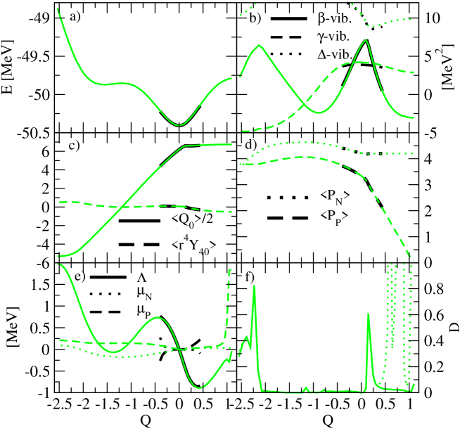
Figure 1: (Color online) Large amplitude collective motion in ⁵⁸Fe with axial symmetry (following the $\beta$-vibration, the second lowest RPA solution at equilibrium). a) Energy along the collective path. b) The square of the lowest RPA frequencies. c) The dimensionless quadrupole moment, $\left<Q_{0}\right>$, and the hexadecapole moment, $\left<r^{4}Y_{40}\right>$. d) The dimensionless pairing operators $\left<P_{\tau}\right>$. e) The cranking parameter $\Lambda$ and the chemical potential $\mu$. f) The decoupling measure, $D$. The dotted line represents the numerically over-complete decoupling measure and the solid line the correct calculation where the contribution due to over-completeness of the projection basis has been removed. The grey (green online) curves represents the results for the projected RPA and the black curves are for the full RPA.

We first investigate axial collective motion (see also AW03 ), by following the $\beta$-vibration (even though this is not the lowest eigenvalue at equilibrium, it is the lowest one of axial symmetry). From Fig. 1 we can see that the quadrupole moment is approximately proportional to the collective coordinate $Q$ in the region $-2<Q<0$, which is an indication that we have a path relative close to what we would obtain from a mean-field calculation with a constraint on the quadrupole moment. At larger and smaller values of $Q$ the deformation $\left<Q_{0}\right>$ remains almost constant. Instead, the collective coordinate is now dependent on the pairing fields, for large $Q$ proton pairing and for small $Q$ neutron pairing. At $Q\approx 1.1$ the proton pair field collapses to zero. Our collective path ends at this point, since the singularity at zero pairing is similar to the origin in polar coordinates, with $Q$ playing the role of radial coordinate and the pairing phase $\phi$ the role of polar angle. The change from quadrupole to pairing mode is dominated by a narrowly avoided crossing with the lowest pairing-vibration at $Q\approx 0.2$. After this crossing the quadrupole moment, $\left<Q_{0}\right>$ saturates and the $\left<P_{p}\right>$ starts changing. This avoided crossing shows that more then one collective coordinate would be needed for an accurate description of the collective dynamics. The RPA frequency of the $\beta$-vibration is as expected proportional to the derivative of the cranking parameter, $\Lambda$.

We have also looked at the potential energy, simply calculated as the expectation value of the Hamiltonian at each point. In Fig. 1 a) we see that the potential has a local energy maximum at $Q\approx-1$, which corresponds to a spherical shape, and a shallow oblate minimum at $Q\approx-1.6$. The potential around the minimum show an a quadratic behaviour which indicates that the harmonic approximation in RPA is well fulfilled for small-amplitude collective motion, but obviously fails for wave functions that have substantial support away from the minimum. It can easily be seen that the regions where the potential energy has a positive derivative are the regions where the cranking parameter, $\Lambda$, has negative value and the converse.

The key to the whole approach is the decoupling parameter, $D$, which is plotted in Fig. 1 f). It has a small value indicating a good decoupling of the collective mode from all the non-collective modes. The exceptions are at $Q\approx 0.2$ and $Q<-2$ which is due to two avoided crossings of the $\beta$-vibration with the pairing vibrations, as can be seen in Fig. 1 b). The large peak in Fig. 1 f) at $Q>0.5$ is due to an approximate numerical over-completeness in in the basis on which we have projected the RPA vectors. The over-completeness comes when a pair field is zero and the projected mass matrix has a zero eigenvalue. This is due to the extra pairing term included in the basis in section III.2. The over-completeness appear near the collapse of the proton pairing field, as can be seen in Fig. 1 d). Even tough the basis only becomes exactly over-complete at the point of pairing collapse the calculation of $D$ is already influenced when the pair field is small, due to the fact the $D$ is calculated from an inverse of the mass matrix (see Eq. (24)) which becomes ill defined. We should of course remove such a spurious contribution; this can be done quite easily, and leads to the result plotted as a solid curve in Fig. 1 f). From now on we will only plot the value of $D$ where the contribution from over-completeness has been removed. The collapse of the pair field has a surprisingly strong influence on the collective path. Whether this is a result of the approximations we made, our choice of force or a general feature is not clear at this point.

In section II.4 it was described how to solve the one-body Schrödinger equation for the collective path. In the case discussed above the proton pair field collapses at $Q\approx 1.1$. We can therefore expect that proton pairing rotation will play a key role for the excitation spectrum of our system. The proton pairing mass is plotted in Fig. 2. We can see that close to the collapse of the proton pairing $B_{\phi_{P}}\propto(Q-Q_{\rm max})^{2}$ which is what we expect when the collective coordinate is approximately $\left<P_{P}\right>$. For negative $Q$ $B_{\phi_{P}}$ has a non-trivial behaviour.

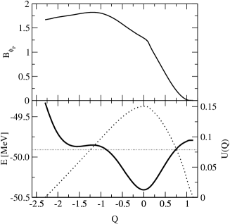
Figure 2: The upper panel show the proton rotational mass along the collective path for projected axial large amplitude collective motion in ⁵⁸Fe (following the second RPA solution). The lower panel show energy and the radial wave function for the large amplitude collective motion in ⁵⁸Fe, following the second RPA solution. The thick solid line is the potential energy, the thin horizontal line give the position of the lowest eigenvalue. The energy scale is on the left side. The wave function is shown as well (dotted line), with the scale on the right side.

In Fig. 2 we also show the lowest eigenvalue and radial wave function of the collective Hamiltonian including $k=0$ proton pairing rotation. At $Q=Q_{\rm max}$ where $B_{\phi_{P}}=0$ the ground-state wave-function goes to zero linear in $Q$ as expected from at the origin in polar coordinates. At $Q=Q_{\rm min}$ we have made the approximation that $U(Q_{\rm min})=0$. There is no bound state supported by the shallow oblate minimum and the lowest excited state is $1.30$ MeV above the collective ground state. This excitation energy is substantially smaller then the RPA harmonic approximation energy of $2.54$ MeV and reflects the anharmonic nature of the large-amplitude excitation. In table 4 we can see that the large component of the wave-function at small and negative $Q$ gives rise to a reduction of the expectation value of $Q_{0}$ by almost 30% relative to the mean-field results.

Table 4: The expectation values of the quadrupole- and pairing operators for $k=0$ collective Hamiltonian along the axial collective path in ⁵⁸Fe and at the mean-field minimum.

	$Collective$	$Mean-field$
$\left<Q_{0}\right>$	$8.98$	$12.37$
$\left<P_{N}\right>$	$4.36$	$4.21$
$\left<P_{P}\right>$	$3.25$	$3.34$

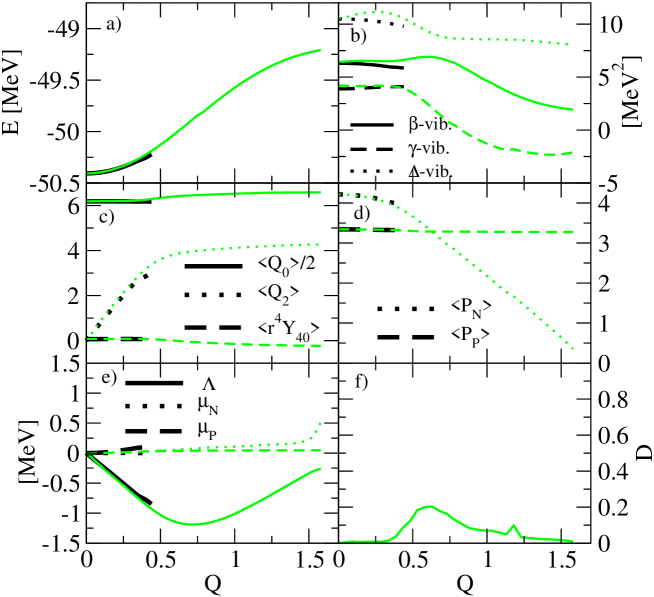
Figure 3: (Color online) Large amplitude collective motion in ⁵⁸Fe (following the $\gamma$-vibration, the lowest RPA solution at equilibrium). a) Energy along the collective path. b) The square of the lowest RPA frequencies. c) The dimensionless quadrupole moments, $\left<Q_{0}\right>$, $\left<Q_{2}\right>$ and the hexadecapole moment, $\left<r^{4}Y_{40}\right>$. d) The dimensionless pairing operators $\left<P_{\tau}\right>$. e) The cranking parameter $\Lambda$ and the chemical potential $\mu$. f) The decoupling measure, $D$. The grey (green online) curves are the results for the projected RPA and the black curves are for the full RPA.

In the case where we follow the path emerging from the lowest mode, the $\gamma$-vibration, we can obtain similar results. A number of results identifying the collective path are shown in Fig. 3, where we have linear change of $\left<Q_{2}\right>$ with the collective coordinate, while all other expectation values remain relatively unchanged for $|Q|<0.5$. At larger values of the collective coordinate we see a saturation in $\left<Q_{2}\right>$ and a strong reduction in the neutron pair field, which finally collapses to zero. Once again, this is mediated by an avoided crossing between quadrupole- and pairing-vibration modes. The decoupling measure, $D$, in Fig. 3 f) has a similar behaviour as for the $\beta$-vibration. The crossing with the pairing vibration is visible as an increase in $D$ at around $Q\approx 0.6$. At larger $Q$ we have a large contributions to $D$ due to over-completeness of the basis this time caused by the strongly reduced neutron pairing field. By mirroring the potential to negative $Q$ (and negative $\left<Q_{2}\right>$) we get a closed collective path from the neutron pairing collapse at $Q\approx 1.6$ to the mirrored neutron pairing collapse at $Q\approx-1.6$. The neutron rotational pairing mass in Fig. 4 shows the expected quadratic behaviour in $\left|Q\right|$ close to $Q_{\rm max}$.

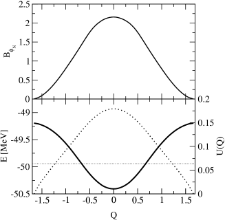
Figure 4: The upper panel show the proton rotational mass along the collective path for projected large amplitude collective motion in ⁵⁸Fe (following the lowest RPA solution). The lower panel show energy and the radial wave function for the large amplitude collective motion in ⁵⁸Fe, following the lowest RPA solution. The thick solid line is the potential energy, the thin horizontal lines give the position of the lowest eigenvalue. The energy scale is on the left side. The wave function is shown as well (dotted line), with the scale on the right side.

In Fig. 4 we also show the eigenvalues and wave-functions of the collective Hamiltonian including $m=0$ neutron pairing rotation. The lowest excited state is at $1.49$ MeV above the collective ground state. This excitation energy is substantially smaller then the corresponding RPA excitation energy of $2.05$ MeV. This again is a result of the anharmonic nature of the collective potential. In table 5 we can see that the lowest state has a substantially reduced value of $\left<P_{N}\right>$ compared to the mean-field value at the minimum.

Table 5: The expectation values of the quadrupole- and pairing operators for $m=0$ collective Hamiltonian along the non-axial collective path in ⁵⁸Fe and at the mean-field minimum.

	$Collective$	$Mean-field$
$\left<Q_{0}\right>$	$12.63$	$12.37$
$\left<P_{N}\right>$	$3.53$	$4.21$
$\left<P_{P}\right>$	$3.31$	$3.34$

III.4 Realistic application of large amplitude collective motion

The case of ⁵⁸Fe has the advantage that the configuration space is relatively small and therefor there are no big computational problems, and we could compare exact and approximate solutions. It still allows us to explore several key features of our method and test its feasibility and the quality of the results. To test the method in more realistic circumstances we decided to apply our method to the rare-earth region. We have chosen ¹⁵⁶Gd and ¹⁸²Os since the gadolinium nucleus is known to be $\beta$-soft, whereas the osmium isotope is $\gamma$-soft. Both nuclei are situated in a region which is rich in nuclear structure phenomena.

The calculations for ¹⁵⁶Gd and ¹⁸²Os are done in a configuration space consisting of the $N=5(4)$ and $6(5)$ neutron(proton) shells. The spherical single particle energies and suppression factors of Eq. (53) and (54) are again taken from BK68 . We compare the RPA energies and the RPA vectors calculated with the full RPA and using the projected approximation in table 6.

Table 6: Comparison of the full RPA energy, $\hbar\Omega$, the projected RPA energy, $\hbar\bar{\Omega}$, and $\delta_{B,1}$ for the $\beta$-, $\gamma$-, $\Delta^{(1)}$- and $\Delta^{(2)}$-vibrations in case of ¹⁵⁶Gd and ¹⁸²Os using the new projection basis (57). The energies are in units of MeV.

	156Gd
	$\hbar\Omega$	$\hbar\bar{\Omega}$	$\delta_{B}$	$\delta_{1}$
$\beta$-vibration	$0.8850$	$0.9224$	$0.0040$	$0.5138$
$\gamma$-vibration	$1.6860$	$1.8490$	$0.0366$	$0.0325$
$\Delta^{(1)}$-vibration	$1.8089$	$1.8147$	$0.0049$	$0.0042$
$\Delta^{(2)}$-vibration	$1.9923$	$2.2256$	$0.9409$	$0.9339$
	182Os
	$\hbar\Omega$	$\hbar\bar{\Omega}$	$\delta_{B}$	$\delta_{1}$
$\beta$-vibration	$1.5704$	$1.5851$	$0.0058$	$0.0087$
$\gamma$-vibration	$1.1208$	$1.1458$	$0.0016$	$0.0010$
$\Delta^{(1)}$-vibration	$1.6690$	$1.6776$	$0.0106$	$0.0147$
$\Delta^{(2)}$-vibration	$1.8476$	$2.0673$	$0.2165$	$0.2826$

We find a good agreement for the low-lying solutions. The second pairing vibration is somewhat too high in energy which is also reflected in a small overlap of the RPA vectors. The projection basis seems to work very well in the cases of heavier nuclei and larger configuration spaces examined here.

In Fig. 5–7 we can see the results of the large amplitude collective motion following the lowest axial symmetric solution. We have included both the results obtained with the full RPA as well those employing the RPA projected on a basis.

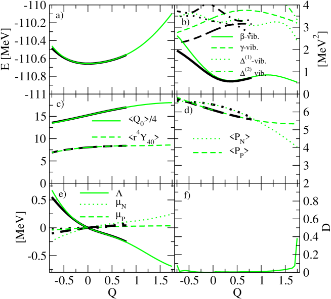
Figure 5: (Color online) Axial collective motion in ¹⁵⁶Gd. See Fig. 1 for more details.

In ¹⁵⁶Gd the lowest solution is the $\beta$ vibration but it also has quite large pairing components, as can be seen in Fig. 5 in the change in strength of the pair fields. There is in general a non-trivial structure of the collective path close to the mean-field minimum which also can be seen in Fig. 5 a) where the energy show anharmonic behaviour around the minimum. Figure 5 f) show a good decoupling of the collective degrees of freedom from the non-collective degrees of freedom in the region close to the minimum.

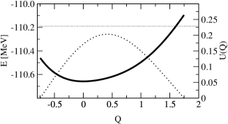
Figure 6: The energy along the collective path for projected axial large amplitude collective motion in ¹⁵⁶Gd (following the first RPA solution) is drawn with the thick solid line with the energy scale on the left side. The lowest eigenvalue of the Hamiltonian is drawn as a thin horizontal line. The corresponding eigenfunction has the scale on the right side.

In Fig. 6 we can see that there is one low-lying solution of the collective Hamiltonian. The fact the lowest eigenvalue is situated high in energy, relative to the range in which we have found the collective potential, tells us that the assumption that $U(Q)=0$ at the at the ends of the collective path is not justified in this case. One can expect that the correct $U$ would stretch substantially outside the range on which we have calculated the collective path.

¹⁸²Os is a $\gamma$-soft nucleus and we show the result following the 2 lowest normal modes.

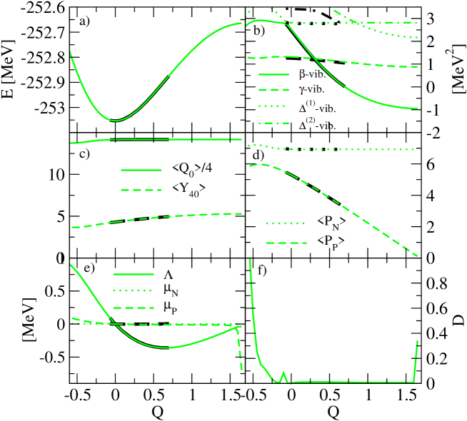
Figure 7: (Color online) Axial collective motion in ¹⁸²Os. See Fig. 1 for more details.

In Fig. 7 we can see that the lowest axial RPA solution is mainly of proton pairing nature. The strength of the proton pair field is proportional to the collective coordinate and that the pair field collapses at $Q\approx 1.6$ which leads to a jump in the chemical potential. For small negative values of $Q$ there is an avoided crossing with a mode that is dominantly a shape vibration, which leads to a reduction of $\left<Q_{0}\right>$. The energy along the collective path in Fig. 7 a) show a maximum when $\left<P_{P}\right>\rightarrow 0$ and a approximately harmonic behaviour around the minimum. Figure 7 f) shows a good decoupling of the collective degrees of freedom from the non-collective degrees of freedom in the region close to the minimum. At large negative values of $Q$ we have a crossing with a proton paring vibration which gives large state mixing and therefore no decoupling of the collective solution.

Fig. 8 show the results when following the collective path defined by the lowest $\gamma$-vibration in ¹⁸²Os.

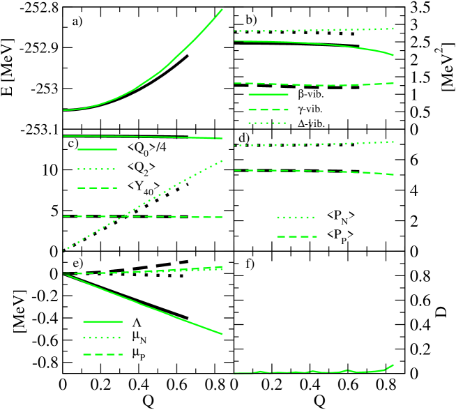
Figure 8: (Color online) Non-axial collective motion in ¹⁸²Os. See Fig. 3 for more details.

The calculation shows that the collective path is mainly dominated by the increase of the $\left<Q_{2}\right>$ tri-axial deformation. At $Q>0.8$ we see an avoided crossing of the $\beta$- and $\gamma$-vibration which causes an numerical instability in our calculations. This also signals the need for more then one collective coordinate. Even though there are numerical difficulties in implementing our method in some cases we can see that our projection method works very well in the larger configuration spaces employed here and it is practically implementable.

IV Conclusions and summary

We have extended the method of calculating the self-consistent collective path presented in DK00 to include constraints on the particle number and implemented it for the quadrupole+pairing Hamiltonian BK68 . The method consists of finding a series of points fulfilling the force equation, where the local direction of the collective path is determined in each point by the local normal modes. The local RPA equations and the force equation are solved in a double iterative process with constraints on the particle numbers and the step length along the collective path. The method allows us to determine the collective coordinate from the Hamiltonian without having to assume a priori which are the relevant degrees of freedom.

To implement this method in heavier systems and for more realistic nuclear forces we need to truncate the RPA calculation in a way that will give an accurate approximation of the low-lying RPA solutions. We have improved the projection method originally presented in NW99 in such a way that we are able to describe all low-lying states including pairing vibrations. This is done by expanding the state-dependent basis suggested in NW99 to include a pairing term, which is only active around the Fermi surface. The new basis set gives RPA energies very close to the exact solutions. The calculation of the overlap of the wave functions between the full and our approximate RPA solution shows that the wave functions are almost identical. We can therefore expect our method to give a good approximation to the collective path.

Our method of calculating the collective path has been implemented for the cases of ⁵⁸Fe, ¹⁵⁶Gd and ¹⁸²Os. We have chosen to follow the lowest axially symmetric and tri-axial solutions. The decoupling of our collective coordinate from all the non-collective coordinates can be quantified in the decoupling measure $D$. This is found to be small along the collective path with the exception of regions of avoided crossings where the system undergoes configuration mixing. In such regions one collective coordinate is not sufficient to describe the system accurate. In regions where the projection basis gets over-complete $D$ has to be calculated with special care. This happens when the proton and/or the neutron pairing collapses.

We see that the collective path goes through avoided crossings with pairing solutions in most cases in both ⁵⁸Fe and ¹⁸²Os. This leads to collapses of the pair fields and an end of the collective path. These avoided crossings also show that more then one collective coordinate would be needed for a accurate description of the collective motion. In the $\beta$-soft nucleus ¹⁵⁶Gd the collective coordinate is of a more complicated structure which can also be seen in the non-harmonic shape of the potential energy. Our projected local RPA method for calculating the collective path gives very good agreement with the results obtained using the full RPA. The method is very useful when calculating self-consistent large amplitude collective motion in large a configuration space.

By solving the one-dimensional “radial” Schrödinger equation along the collective path we are able to examine the effect of the collective motion on ground state properties. In cases where the collective path ends with a collapse of the pair field we must include the effect of pairing rotations on the low energy spectrum. It is surprising that almost all our calculations are dominated by states with collapsing pairing; there may well be important lessons in this feature. The reason they occur so frequently is the presence of low-lying configurations without pairing. One might ask whether this is an artifact of our model, and whether larger configuration-spaces with more complicated interactions would behave differently. Such calculations are clearly called for, but we do not expect dramatically different results, since pairing mainly acts in a small region around the Fermi-surface. There is also a slight possibility that the approximations we made in our treatment of spurious admixtures contributes to these effects. The surprising importance of the pairing collapse is the main result of our calculations that is usually not seen in a standard constrained mean-field calculation.

In this paper we have implemented a method to find the adiabatic self-consistent collective path for a nuclei. A technique to truncate the basis in which the RPA equations are solved has been improved and a good agreement between the full and truncated RPA is found. To solve the RPA equations in a limited basis has proven to be a useful and practical way of calculating the collective path within the local harmonic approximation. We intend to apply similar techniques to the interesting problem of collective motion at finite rotational frequency in the near future. It remains to be investigated how we can include the covariant terms in the RPA in a suitable approximation.

Appendix

The six conditions (Eqs. (13) and (19–21)) gives a set of equations which can be solved for the six parameters $\epsilon_{i}^{(n)}$, $\eta_{i\tau}^{(n)}$, $\lambda_{i}^{(n)}$ and $\mu_{i\tau}^{(n)}$ for each $i$ and $n$. For $i=0$ we get

$$\epsilon_{0}^{(n)} = \frac{\Delta Q}{1+\frac{f^{(0)}\cdot f^{(n)}}{f^{(n)}\cdot f^{(n)}}-\sum_{\tau}\frac{N^{20(n)}_{i\tau}\cdot f^{(n)}}{f^{(n)}\cdot f^{(n)}N^{20(n)}_{i\tau}\cdot N^{20(n)}_{i\tau}}\left(f^{(0)}+f^{(n)}\right)\cdot N^{20(n)}_{i\tau}},$$ (61)

$$\eta_{0\tau}^{(n)} = -\epsilon^{(n)}_{0}\frac{f^{(n)}\cdot N^{20(n)}_{i\tau}}{f^{(n)}\cdot f^{(n)}}.$$ (62)

For all other $i$ Eqs. (16) and (17) together with the constraints (13–21) give

$$\epsilon_{i}^{(n)} = \frac{-\delta^{(n)}_{i}f^{(0)}\cdot\Delta^{(n)}_{\perp i}{\cal R}+\sum_{\tau}\frac{N^{20(n)}_{i\tau}\cdot\Delta^{(n)}_{i-1}{\cal R}}{N^{20(n)}_{i\tau}\cdot N^{20(n)}_{i\tau}}\left(f^{(0)}+f^{(n)}\right)\cdot N^{20(n)}_{i\tau}}{1+\frac{f^{(0)}\cdot f^{(n)}}{f^{(n)}\cdot f^{(n)}}-\sum_{\tau}\frac{N^{20(n)}_{i\tau}\cdot f^{(n)}}{f^{(n)}\cdot f^{(n)}N^{20(n)}_{i\tau}\cdot N^{20(n)}_{i\tau}}\left(f^{(0)}+f^{(n)}\right)\cdot N^{20(n)}_{i\tau}},$$ (63)

$$\eta_{i\tau}^{(n)} = -\epsilon^{(n)}_{i}\frac{f^{(n)}\cdot N^{20(n)}_{i\tau}}{f^{(n)}\cdot f^{(n)}}-N^{20(n)}_{i\tau}\cdot\Delta^{(n)}_{i-1}{\cal R},$$ (64)

$$\lambda^{(n)}_{i} = \frac{H^{20(n)}_{i}\cdot f^{(n)}-\sum_{\tau}\frac{H^{20(n)}_{i}\cdot N^{20(n)}_{i\tau}N^{20(n)}_{i\tau}\cdot f^{(n)}}{N^{20(n)}_{i\tau}\cdot N^{20(n)}_{i\tau}}}{f^{(n)}\cdot f^{(n)}-\sum_{\tau}\frac{\left(N^{20(n)}_{i\tau}\cdot f^{(n)}\right)^{2}}{N^{20(n)}_{i\tau}\cdot N^{20(n)}_{i\tau}}},$$ (65)

$$\mu^{(n)}_{i\tau} = \frac{H^{20(n)}_{i}\cdot N^{20(n)}_{i\tau}-\lambda^{(n)}_{i}f^{(n)}\cdot N^{20(n)}_{i\tau}}{N^{20(n)}_{i\tau}\cdot N^{20(n)}_{i\tau}}.$$ (66)

These equations can easily be generalised to incorporate additional constraint operators like angular momentum. They are slightly more complicated than those shown in other work DK00 , since we have chosen to fix the step size in the collective coordinate.

References

- (1) Tunneling in complex systems edited by S. Tomsovic, (World Scientific, Singapore; London, 1998)
- (2) G. Do Dang, A. Klein and N.R. Walet, Phys. Rep. 335, 93–274 (2000)
- (3) W.H. Bassichis, A.K. Kerman and J.P. Svenne, Phys. Rev. 160, 746 (1967)
- (4) P. Ring and P. Schuck, The Nuclear Many-Body Problem, (Springer, New York, 1980)
- (5) M. Kobayasi, T. Nakatsukasa, M. Matsuo and K. Matsuyanagi, nucl-th/0304051
- (6) T. Nakatsukasa, N.R. Walet and G. Do Dang, Phys. Rev. C 61, 014302 (1999)
- (7) M. Barranger and K. Kumar, Nuc. Phys. A110, 490 (1968)
- (8) V.O. Nesterenko, J. Kvasil and P.-G. Reinhard, Phys. Rev. C 66, 044307 (2002)
- (9) T. Nakatsukasa and N.R. Walet, Phys. Rev. C 58, 3397 (1998)
- (10) G. Holzwarth, Nucl. Phys. A113, 448 (1968); Nucl. Phys. A133, 161 (1969)
- (11) R. Abraham, J.E. Marsden and T. Ratiu, Manifolds, Tensor Analysis, and Applications (Second Edition) (Springer-Verlag, New York, 1988)
- (12) P. Möller, J.R. Nix, W.D. Myers and W.J. Swiatecki, Atomic Data and Nuclear Data Tables, Vol. 59, No. 2, 185-381 (1995)
- (13) P. Möller and J.R. Nix, Nucl. Phys. A536, 20 (1992)
- (14) D. Almehed and N.R. Walet, Acta Phys. Pol. B 34, 2227(c) (2003)
- (15) S.G. Nilsson, Mat. Fys. Medd. Dan. Vid. Selsk. 29, no. 16 (1955)
- (16) S.G. Nilsson and I. Ragnarsson, Shapes and Shells in Nuclear Structure (Cambridge University Press) (1995)