Quantum Monte Carlo Calculations of Neutron Matter

Abstract

Uniform neutron matter is approximated by a cubical box containing a finite number of neutrons, with periodic boundary conditions. We report variational and Green’s function Monte Carlo calculations of the ground state of fourteen neutrons in a periodic box using the Argonne $v8^{\prime}$ two-nucleon interaction at densities up to one and half times the nuclear matter density. The effects of the finite box size are estimated using variational wave functions together with cluster expansion and chain summation techniques. They are small at subnuclear densities. We discuss the expansion of the energy of low-density neutron gas in powers of its Fermi momentum. This expansion is strongly modified by the large $nn$ scattering length, and does not begin with the Fermi-gas kinetic energy as assumed in both Skyrme and relativistic mean field theories. The leading term of neutron gas energy is $\sim$ half the Fermi-gas kinetic energy. The quantum Monte Carlo results are also used to calibrate the accuracy of variational calculations employing Fermi hypernetted and single operator chain summation methods to study nucleon matter over a larger density range, with more realistic Hamiltonians including three-nucleon interactions.

PACS: 21.65.+f,  26.60.+c

I Introduction

Since the discovery of neutron stars in 1967 there has been a continued interest in calculating the properties of neutron matter from realistic models of nuclear forces PR95 ; HP00 . It is difficult to extrapolate the data on bound nuclei using energy-density functionals to estimate the equation of state $E(\rho)$ of pure neutron matter. Various Skyrme and relativistic energy-density functionals which fit the binding energies and radii of nuclei available in laboratories at present give rather different $E(\rho)$ for neutron matter. These energy-density functionals also predict different properties of nuclei near the neutron drip line WNX , which may be synthesized in the near future using radioactive ion beams. Theoretical predictions of the neutron matter $E(\rho)$ have been used to constrain the energy density functionals used to study neutron rich nuclei.

The two-neutron interaction is strong and highly spin dependent. Therefore calculating the neutron matter $E(\rho)$ is a challenging many-body problem, though in some ways it is simpler than that of symmetric nuclear matter. Neutron matter properties have been calculated recently with Brueckner theory Engvik97 ; BBB97 and with variational methods using chain summation techniques WFF88 ; APR98 . There is good agreement between the results of these two methods HP00 , and recent high precision models of $nn$ interaction give rather similar neutron matter $E(\rho)$ with the lowest order Brueckner method Engvik97 . The results for symmetric nuclear matter, however, have more model dependence. The $E(\rho)$ of high density neutron matter is also sensitive to the lesser known three neutron interaction APR98 .

The Brueckner and variational methods use different expansions. From the results of two- and three-hole line contributions, the cluster expansion in Brueckner theory appears to converge SBGL98 , though contributions of clusters with more than three neutrons have not been calculated. In contrast, the cluster expansion of the energy expectation value of neutron matter used in the variational method has a rather poor convergence when the optimum variational wave function, $\Psi_{V}$ is used. In the latest calculations MPR02 two- and three-body cluster contributions are calculated accurately, while those of $\geq 4$-body clusters are summed approximately with hypernetted and single-operator chain summation methods. The convergence rate of the expansion is sensitive to the range of correlations in $\Psi_{V}$. Hence it is often possible to use shorter range correlations, which give a more convergent cluster expansion together with a variational energy within a few % of the optimum minimum. Thus, even though the results of these two methods are in agreement within several %, the theoretical error in the treatment of long range correlations is not well estimated.

In the past few years it has been possible to calculate the energies of all the bound states of nuclei having up to ten nucleons with errors estimated to be $\lesssim$ 2 % using the Green’s function Monte Carlo (GFMC) method WPCP00 ; PWV02 . Results of these calculations are being used to construct realistic models of three-nucleon interactions PPWC01 . The computational effort necessary for a nuclear GFMC calculation scales approximately with $2^{A}A!/(N!Z!)$ for a system with $N$ neutrons, $Z$ protons and $A=N+Z$. The factor $2^{A}$ comes from the number of spin states of $A$ nucleons and $A!/(N!Z!)$ is the number of charge conserving isospin states. In the present work we report calculations of the ground state of 14 neutrons in a periodic box (PB) with the GFMC method considering all the $2^{14}$ spin states. We have also used the auxiliary field diffusion Monte Carlo (AFDMC) method proposed by Schmidt and Fantoni SF99 to calculate the ground state energy. In this method one effectively samples the $2^{14}$ spin states stochastically. The computational effort of AFDMC scales with $A^{3}$, and thus it can be used to study systems with larger values of $A$ FSS01 . The present AFDMC calculations seem to have larger errors than the GFMC; however, it may be possible to improve their accuracy.

The interactions and the variational wave functions used in this work are described in sect. II. The quantum Monte Carlo calculations, variational (VMC), GFMC and AFDMC, are described briefly in section III, where we present results at $\rho=0.04,~{}0.08,~{}0.16$ and 0.24 fm^-3. The details of these methods have been presented previously; here we simply describe the additional techniques used to calculate results for 14 neutrons in a PB, and discuss several tests of the calculations. The total energy and the potential energy expectation values are reported for each density.

The variational calculations using chain summation methods (VCS) are reported in section IV. In this section we also discuss the difference between the density matrices of 14 neutrons in a PB and of uniform gas (UG) with large number of neutrons. The smallness of this difference makes the 14-particle PB a useful approximation to UG. The difference between the energy per neutron in the PB and in UG is estimated using variational wave functions. It is small at subnuclear densities, $\rho\leq\rho_{0}=0.16$ fm^-3, but significant at 1.5 $\rho_{0}$. The comparison of VCS results with the QMC suggests that the former can have errors up to $\sim$ 10 %.

The pair distribution functions obtained from VMC and GFMC calculations are compared in section V. These indicate that neutron matter has strong correlations even at small densities, as expected from the large scattering length, $a\sim-18$ fm in the ${}^{1}S_{0}$ state. The results for the $E(\rho)$, extrapolated to the UG limit, are presented in section VI. Here we also discuss the expansion of the $E(\rho)$ in powers of $k_{F}$. When $|ak_{F}|<1$, this expansion begins with the Fermi-gas kinetic energy, $T_{FG}=0.3k_{F}^{2}/m$. However, at densities of interest in nuclear or neutron star physics $|ak_{F}|>>1$, and the expansion of the $E(\rho)$ seems to begin with $\sim T_{FG}/2$, which is the estimated UG energy for a short range interaction with scattering length $(-a)\rightarrow\infty$. This approximation to nuclear forces in low-density neutron-gas was suggested by Bertsch Bertsch .

The accuracy of the present calculation is discussed in the last section VII. At densities $\leq\rho_{0}$ the GFMC calculation appears to be well converged and presumably has an accuracy of $\sim 2$ % for the energy of normal neutron matter. However, there is exceptionally strong pairing in dilute Fermi gases with $ak_{F}\rightarrow-\infty$ ERS97 , and their superfluid state can have energies below those of the normal state by $\sim$ 10 % dfg . The main error in the predicted energy of low density neutron matter, where three-body forces are small, is likely to be due to the neglect of the superfluidity in the present calculation.

II Interactions and Variational Wave Functions

We have used the Argonne $v8^{\prime}$ two-nucleon interaction PPCPW97 in this work. This simplified interaction equals the isoscalar part of the realistic Argonne $v18$ interaction in all the S- and P-waves as well as in ${}^{3}D_{1}$ and its coupling to ${}^{3}S_{1}$. In neutron matter this interaction can be written as an operator with four terms:

$$v_{ij} = \sum_{p=1,4}v_{p}(r_{ij})O^{p}_{ij}~{},$$ (1)

$$O^{p=c,\sigma,t,b}_{ij} = 1,~{}\mbox{\boldmath$\sigma$}_{i}\cdot\mbox{\boldmath$\sigma$}_{j},~{}S_{ij},~{}{\bf L}\cdot{\bf S}~{}.$$ (2)

Here $S_{ij}$ and ${\bf L}\cdot{\bf S}$ are the usual tensor and spin-orbit operators. In the calculations using the PB boundary condition, the interaction is truncated at $r_{ij}=L/2$, where $L$ is the length of the cubic box holding 14 neutrons $(L^{3}\rho=14)$ :

$$v(r_{ij})=v(r_{ij})~{}\theta(\frac{L}{2}-r_{ij})+v(r_{ij})~{}\theta(r_{ij}-\frac{L}{2})~{}.$$ (3)

The contribution of the long range part, $v(r_{ij})~{}\theta(r_{ij}-\frac{L}{2})$, to the $E(\rho)$ of UG is estimated using variational calculations. While at low densities this contribution is small, at $\rho=0.24$ fm^-3 it becomes comparable to the total $E(\rho)$ in magnitude.

The variational wave function $\Psi_{V}$ used in this work has the form:

$$\Psi_{V}=\left({{\cal S}}\prod_{i<j}F_{ij}\right)\Phi~{},$$ (4)

where $\Phi$ is the noninteracting Fermion wave function. In UG calculations $\Phi=\Phi_{FG}$, the Fermi-gas wave function, while in calculations using the PB boundary conditions $\Phi=\Phi_{PB}$. It has 14 neutrons occupying spin up and down states with momenta

$${\bf k}=0,~{}\pm k_{B}\hat{\bf x},~{}\pm k_{B}\hat{\bf y},~{}\pm k_{B}\hat{\bf z}~{}.$$ (5)

Here $k_{B}=2\pi/L$ and $\hat{\bf x},\hat{\bf y}$ and $\hat{\bf z}$ are unit vectors.

The ${{\cal S}}\prod$ denotes a symmetrized product of the noncommuting $F_{ij}$ pair correlation operators. In VCS calculations they have four terms involving the four operators of Eq. (2):

$$F_{ij}=\sum_{p=c,\sigma,t,b}\beta_{p}~{}f_{p}(r_{ij})O^{p}_{ij}~{}.$$ (6)

The correlation functions $f_{p}(r_{ij})$ are obtained by solving two-body Schrödinger-like equations WFF88 , and have three parameters, $d,d_{t}$ and $\alpha$. They correspond to the range of all but the tensor correlations $(d)$, range of tensor correlations $(d_{t})$, and the average quenching of spin-dependent interactions in matter $(\alpha)$.

In the case of UG, the values of $d,~{}d_{t}$ and $\alpha$ are determined by minimizing the energy with the VCS method for $\beta_{p}=1$. Constraints imposing conservation of nucleons are used during this minimization WFF88 to prevent the $F_{ij}$ from going into regions where the chain summation approximation fails. The parameters $\beta_{\sigma},~{}\beta_{t}$ and $\beta_{b}$ provide additional variation of $F$; $\beta_{c}$ is not a variational parameter since $F(r_{ij}\rightarrow\infty)=1$. The $\beta_{p\neq c}$ parameters were not used in recent calculations APR98 since they do not lower the energy significantly after optimizing $d,~{}d_{t}$ and $\alpha$. They are used here for the following reason. The optimum values of $d$ and $d_{t}$ in UG are $>L/2$. However, in VMC as well as VCS calculations using the PB boundary condition the $d$ and $d_{t}$ must be $\leq L/2$. In all PB calculations we use $d=d_{t}=L/2$, and vary the $\alpha$ and $\beta_{p\neq c}$ to minimize the energy.

In VMC calculations the spin-orbit correlations in the $F_{ij}$ are neglected due to computational difficulties associated with the gradient operator in ${\bf L}$. These calculations use the $v6$ interaction obtained by dropping the spin-orbit term in the $v8^{\prime}$. There results are compared with those of VCS with the same $F$ to test the accuracy of the chain summation approximation. The complete $v8^{\prime}$ interaction is used in the GFMC calculations where the spin-orbit correlations are generated by propagation in imaginary time as discussed in the next section.

III Quantum Monte Carlo Calculations

Quantum Monte Carlo methods have often been used to study infinite systems of either fermions or bosons at both zero and finite-temperature. Examples include atomic liquid ³He and ⁴He lheqmc , the electron gas, egasqmc as well as a myriad studies of lattice models in condensed matter theory. They have proven remarkably successful at studying the equation of state of strongly-interacting systems, and have also been used to explore phase transitions, momentum distributions, static and dynamic response, etc. Although studies of fermion systems are usually treated via approximate fixed-node fixednode or constrained path (CP) constrainedpath methods, these approximations can often be quite accurate.

The nuclear many-body problem is more difficult than all the cases listed above, because of the strong spin-isospin dependence of the interaction. Instead of a single function of the 3A coordinates of the particles, the wave function of simple systems, the nuclear state is described with a set of (complex) amplitudes dependent upon the spins and isospins of the nucleons. This complexity has been handled successfully for few-body (A $\leq$ 10) nuclei PWV02 by simply summing explicitly over all these amplitudes. Monte Carlo is then used to evaluate the 3A-dimensional spatial integrals.

Variational Monte Carlo (VMC) calculations evaluate the energy and other observables through the use of the Metropolis Monte Carlo method. The method is described in detail in WPCP00 , the basic idea being to generate points in the 3A-dimensional configuration space distributed with the probability density of a weight function $W({\bf R})$. Here ${\bf R}$ is the 3A-dimensional configuration vector ${\bf r}_{1},...{\bf r}_{A}$. The expectation values of operators are obtained as averages over the sampled points ${\bf R}_{i}$:

$$\langle O\rangle=\frac{\sum_{i}\langle\Psi({\bf R}_{i})|O|\Psi({\bf R}_{i})\rangle/W({\bf R}_{i})}{\sum_{i}\langle\Psi({\bf R}_{i})|\Psi({\bf R}_{i})\rangle/W({\bf R}_{i})}.$$ (7)

The optimum weight function in most cases is the square of the wave function $\langle\Psi({\bf R})|\Psi({\bf R})\rangle$ for which the denominator of $\langle O\rangle$ has zero variance. For a system of 14 neutrons the $\langle\Psi({\bf R})|\Psi({\bf R})\rangle$ is a sum of squares of the $2^{14}$ spin amplitudes.

This method grows exponentially in computational time with increasing A, and present-day computers limit practical simulations to roughly 14 neutrons. This is somewhat larger than the largest nuclei handled to date because there is only one isospin component to the wave function. Another limitation of these initial calculations is that we have dropped the $L\cdot S$ pair correlation functions, as they depend upon the momentum of the particles in the pair. A complete evaluation of these terms would be difficult because the derivative operators in one pair correlation function can, in principle, act on all other pair correlations. This limitation is not very important at low densities, but can be quite significant at higher densities. The variational wave function cannot adequately describe p-wave pairing of the neutrons which appears to be important at nuclear densities and above. It may be possible to construct a simplified wave function which includes most of these correlations in the future.

Green’s function Monte Carlo (GFMC) methods are then used to obtain the ground-state energy and other properties for the 14 neutrons with periodic boundary conditions. The method is the same as that used for light nuclei WPCP00 , with only very minor modifications used to implement the periodic boundary conditions. The basic idea is to sample a wave function $\Psi(\tau)$ by evaluating path integrals of the form:

$$\Psi(\tau)=\prod\exp[-(H-E_{0})\Delta\tau]|\Psi_{V}>,$$ (8)

where each step in the product evolves the system over a short imaginary time $\Delta\tau$; after many steps $n\rightarrow\infty$, $\Psi(\tau=n\Delta\tau)$ will converge to the true ground state of the system as long as the original (variational) wave function is not orthogonal to it. Because we are studying systems at densities higher than equilibrium nuclear density $\rho_{0}$, the time step used here is 0.00025 MeV^-1, or 1/2 the time step typically used in nuclear calculations. Again the spatial integrals are done with Monte Carlo, using a sum over many configurations with different spatial coordinates $\bf R$. Each configuration includes amplitudes for all the 2¹⁴ spin states which are explicitly summed in the evaluation of matrix elements.

Some of the GFMC results reported here are obtained with the CP approximation constrainedpath ; WPCP00 . Since the neutrons are fermions, they may exchange and produce contributions to the wave function of opposite signs, and indeed with arbitrary complex phases. In an exact GFMC calculation, this leads to a statistical error that grows with $\tau$. This problem is more severe at higher densities (or with larger numbers of particles) since it is then easier for a pair to interchange.

To deal with this problem, we implement a constraint on the paths to be included in the evaluation of $\Psi(\tau)$. For a spin-isospin independent interaction the wave function is a scalar, and one can perform a fixed-node calculation in which configurations where the variational wave function is zero are discarded. This defines a surface within which the evolution proceeds, and eliminates the sign problem at the cost of introducing an approximation into the calculation. The fixed-node method is exact when the variational wave function has the true nodal surface, and provides an upper bound to the true ground state energy. This upper bound is often quite accurate because we are solving for the “optimum” solution subject only to the boundary condition that the wave function is zero on a predefined surface close to the correct one.

The nuclear case is more complex, both because the trial wave function is a set of complex amplitudes and because we cannot evaluate the full wave function for a given set of coordinates. We can only evaluate it for a specific order of pair correlation operators in Eq 4, as a complete set would require $[A(A-1)/2]!$ terms. These pair orders are sampled in both the VMC and GFMC calculations. Fortunately the fluctuations in samples of pair orders arise from the commutators of correlation operators. These involve clusters of three or more nucleons, and they have a small effect on the variance. For the nuclear case, we construct an alternative constraint based on the overlap of each configuration $\Psi(\tau,{\bf R}_{i})$ with the sampled variational wave function. Configurations with negative overlap are discarded along with those with correspondingly small positive overlap, ensuring that the average overlap of the discarded configurations with the trial wave function is zero. This yields a stable simulation, and the calculation can proceed out to quite large imaginary time, much larger than the inverse gap in the system. This approximation is not guaranteed to produce an upper bound to the ground-state energy, though it has proven to be quite accurate for few-body nuclei. The results obtained using this method are labeled with CP.

The CP approximation is tested by removing the constraint. The configurations generated by the CP calculation are evolved further in the imaginary time $\tau$ without constraint. The fermion sign problem makes this calculation more difficult for increasing density and for increasing $\tau$. In principle we can evaluate the energy for a much larger $\tau$ at low density. In practice the low-density calculations appear to be well converged at fairly small imaginary time. Of course the total unconstrained imaginary time propagation is quite small here, typically 0.005 MeV^-1, and hence only fairly high-energy excitations are removed by this procedure. The results of these unconstrained (UC) GFMC calculations are the most accurate of the presented results.

In this work we use $\tau$ to denote the time after the CP propagation. The CP GFMC propagation starts at a large negative $\tau$ and ends at $\tau=0$. The propagation time of CP GFMC is large enough to ensure convergence; however that of UC GFMC is limited by the growth in statistical errors due to the fermion sign problem.

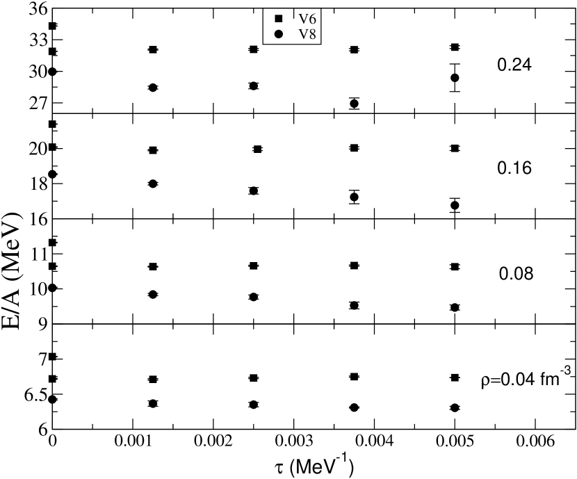
Figure 1: Energy vs. imaginary time $\tau$ after CP propagation, at various densities. VMC results (upper squares) for $v6$ and GFMC-CP results (lower squares and dots) for $v6$ and $v8^{\prime}$ are shown at $\tau=0$, and unconstrained GFMC results are shown for various $\tau>0$.

Results for the VMC and GFMC calculations at different densities are presented graphically in Figure 1. The upper square point at $\tau=0$, at each density, is the VMC results for the $v6$ Hamiltonian, while the lower square point, also at $\tau=0$, shows the CP GFMC results. The CP GFMC energies are typically 5 - 10% lower than the VMC for the $v6$ interaction. The $v6$ VMC and the PB variational chain summation (VCS) calculations discussed in section IV use the same wave function.

The UC GFMC results are plotted as a function of unconstrained propagation time $\tau$ after the end of CP propagation. Circles and squares show results for the $v8^{\prime}$ and $v6$. At all densities, the $v6$ calculations appear to be fairly stable and little change is observed between the CP results and the unconstrained results for larger imaginary time. Table 1 lists the total and potential energy per neutron for various densities. The GFMC potential energies are approximately 15% lower than the VMC results indicating that true ground state has more correlations than the present variational wave function. The difference in the VMC and the GFMC potential energies is more than twice that in the total energies as expected near the minimum. The results of VCS calculations are also listed in Table 1; they are discussed in section IV.

The results for $v8^{\prime}$ interaction are given in Table 2 and Figure 1. The VMC rows in this table give results with the variational wave function for the $v6$ potential without any spin-orbit correlation. With this wave function the expectation value of the spin-orbit interaction, $\langle v_{L\cdot S}\rangle$, is small and positive. It in nonzero due to the tensor correlations. In contrast the variational wave function used in the VCS calculations contain spin-orbit correlations which give significant negative $\langle v_{L\cdot S}\rangle$. The $L\cdot S$ correlations absent in the $v6$ variational wave function are partly generated via the CP propagation as can be seen from the GFMC-CP $\langle v_{L\cdot S}\rangle$ values. However, the constraint imposed by the $v6$ wave function hinders their growth. After the constraint is removed, the spin-orbit correlations increase substantially, and we obtain significantly more attaction from the $v_{L\cdot S}$. This will be more evident in the comparison of pair distribution functions in section VI. The UC GFMC energy decreases with $\tau$ (Fig. 1), and at $\rho\geq\rho_{0}$ the growth in statistical error limits the UC calculation.

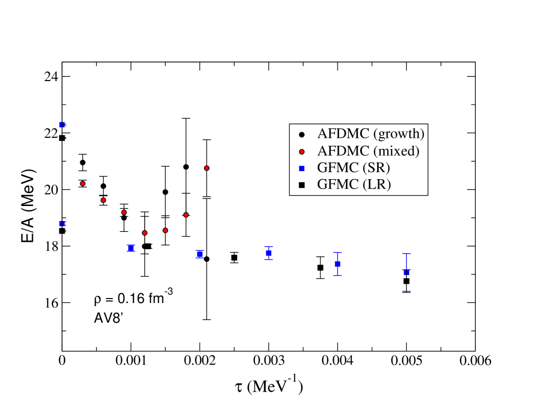
Figure 2: Energy vs. imaginary time $\tau$ for different calculations using $v8^{\prime}$ interaction at $\rho=$ 0.16 fm^-3. Two different estimates (growth and mixed) are shown for the AFDMC calculation along with the results of two different GFMC calculations, using short-range (SR) and long-range (LR) correlations in the trial wave function.

We have also performed calculations with different input correlation functions in the trial wave function. Their results for $\rho=\rho_{0}$ are illustrated by the two sets of square points in Figure 2. The points labeled GFMC(LR) are obtained with the trial wave function having pair correlation functions of range L/2, while those labeled GFMC(SR) have much shorter range input pair correlation functions. There appears to be very little dependence of the UC GFMC results upon the choice of the range of input two-body correlation functions; this has been checked for the pair distribution functions as well.

We have also implemented the auxiliary-field Diffusion Monte Carlo (AFDMC) method of Schmidt and Fantoni SF99 . Since this method scales much better with A than the GFMC method discussed here, it can be used to treat much larger systems. At present the trial wave function used in these calculations includes only spin-independent Jastrow factors times a Fermi-Gas determinant:

$$\Psi_{J}=[\prod_{i<j}f^{c}(r_{ij})]\ \Phi_{FG}.$$ (9)

Each configuration now has 14 two-component vectors describing the relative amplitude and phases of the spin of each neutron. These spins rotate in the presence of fluctuating fields which, when summed, reproduce exactly the results of the two-nucleon interaction. As in the GFMC calculation, a constraint is imposed requiring a positive overlap between the configuration at any time $\tau$ and the trial wave function.

The two sets of UC AFDMC results shown in Figure 2 are obtained with two different estimators of the ground-state energy. The growth energy (black dots) is determined from the rate of increase/decrease in the population with imaginary time $\tau$, while the mixed estimate (red dots) is determined by the overlap of the configurations with the Hamiltonian acting on the trial wave function. These two estimates should be equal within statistical errors for small values of the time step $\Delta\tau$.

The $\Psi_{J}$ is a very simple trial function and hence does not provide an accurate constraint. The CP AFDMC energies at $\tau=0$ are higher than the CP GFMC because of this relatively poor constraint. As $\tau$ increases beyond the CP propagation region, the energy drops and becomes compatible with the GFMC results. The statistical errrors are somewhat worse, though, as each configuration contains only a single set of 14 spin vectors rather than the 2¹⁴ amplitudes in the GFMC. The correlations between these amplitudes reduce the fermion sign problem, but at the cost of an exponentially increasing computational time. The AFDMC method has been used to study much larger systems with this simple constraint, and also to study the spin susceptibility of neutron matter. It could be used to determine the difference between the infinite-particle limit and the results for 14 neutrons. Here, though, we use VCS methods to calculate this difference. In addition, the QMC results provide a test of the VCS calculations often used in studies with more realistic Hamiltonians that include three-nucleon interactions and relativistic corrections.

IV Variational Chain Summation Calculations

In VCS calculations of UG the expectation value of $H-T_{FG}$:

$$E_{V}-T_{FG}=\frac{\langle\Phi_{FG}|[{{\cal S}}\prod_{i<j}F_{ij}](H-T_{FG})[{{\cal S}}\prod_{i<j}F_{ij}]|\Phi_{FG}\rangle}{\langle\Phi_{FG}|[{{\cal S}}\prod_{i<j}F_{ij}][{{\cal S}}\prod_{i<j}F_{ij}]|\Phi_{FG}\rangle}$$ (10)

is expanded in powers of the short range functions $(F_{ij}-1)$ PW79 . The $\Phi_{FG}$ is an eigenstate of the kinetic energy operator $T=-\sum_{i}\nabla_{i}^{2}/2m$ with the eigenvalue $T_{FG}=0.3~{}k_{F}^{2}/m$, hence the terms with $T$ operating on $\Phi_{FG}$ are not included in the expansion. The $n$-body cluster contribution contains all the terms of this expansion having $n$ neutrons.

The leading two-body cluster contribution to the energy of UG of neutrons is given by:

$$E(2b) = \frac{\rho}{2}\int d^{3}r_{ij}~{}C[F(r_{ij})\left(-\frac{1}{m}\nabla^{2}+v(r_{ij})\right)F(r_{ij})]$$ (11)

$$+ \frac{\rho}{2}\int d^{3}r_{ij}~{}C[e_{ij}~{}F(r_{ij})\left(-\frac{1}{m}\nabla^{2}+v(r_{ij})\right)F(r_{ij})]\ell^{2}(r_{ij})$$

$$- \rho\frac{1}{m}\int d^{3}r_{ij}~{}C[e_{ij}~{}F(r_{ij})\mbox{\boldmath$\nabla$}F(r_{ij})]\cdot\ell(r_{ij})\mbox{\boldmath$\nabla$}\ell(r_{ij})~{}.$$

Here $C[...]$ denotes the spin independent part, called the C-part PW79 of the operators inside the square parenthesis, $e_{ij}$ is the spin exchange operator:

$$e_{ij}=-\frac{1}{2}\left(1+\mbox{\boldmath$\sigma$}_{i}\cdot\mbox{\boldmath$\sigma$}_{j}\right)~{},$$ (12)

and $\ell(r)$ is the spatial density matrix:

$$\ell({\bf r})=\frac{1}{A}\sum_{i}e^{i{\bf k}_{i}\cdot{\bf r}}~{},$$ (13)

normalized such that $\ell(r=0)=1$. It is given by the Slater function:

$$\ell(r)=3[sin(x)-x~{}cos(x)]/x^{3}~{};~{}~{}~{}~{}x=k_{F}r~{}.$$ (14)

for the $\Phi_{FG}$.

It is relatively simple to calculate the above 2-body cluster contribution without approximations. All the terms in the 3-body cluster energy except those containing spin-orbit correlations can now be calculated exactly MPR02 . However, all the $\geq 4$-body cluster contributions as well as the 3-body contributions from ${\bf L}\cdot{\bf S}$ correlations are estimated approximately using the chain summation methods.

Results of VCS calculations of the UG are given in Table 3. These are at optimum values of $d$ and $d_{t}$, which generally exceed the $L/2$ of 14 neutron PB. In this case the $E_{V}$ obtained with $\beta_{p}=1$ is within $\sim$ 2 % of the $E_{V}$ with optimum $\beta_{p}$. The contributions of clusters are calculated following MPR02 . The 3- and $\geq 4$-b-static contributions do not include spin-orbit interaction and correlation terms; their contributions are listed in row $\geq 3$-b-${\bf L}\cdot{\bf S}$. The values of 3-b-static contributions calculated with the chain summation approximation are also given in Table 3 for comparison. They are typically within 10 % of the exact values. The listed values of $\geq 4$-b-static contributions include the elementary 4-body circular exchange diagram discussed in Appendix A. It was omitted in previous APR98 ; MPR02 calculations because it is generally small in symmetric nuclear matter. However, this contribution contains the factor $s^{-3}$, where $s=2,4$ is the spin-isospin degeneracy factor in neutron and symmetric nuclear matter. It is relatively larger in neutron matter, and its values are listed in Table 3.

Table 3 clearly shows that the cluster expansion of the $E(\rho)$ has slow convergence. At low densities this is primarily due to the large $nn$ scattering length. With the $v8^{\prime}$ interaction, the the total contribution of clusters with $n\geq 4$ is $\sim$ 30 (10) % of the total energy at $\rho=$ 0.04 (0.16).

Table 4 gives the results for UG variational energy for $d=d_{t}=L/2$ and optimum values of $\alpha$ and $\beta_{p}$. The cluster expansion has better convergence for these shorter range correlations, and the $E_{V}(d=d_{t}=L/2)$ is above the optimum $E_{V}$ by only $\sim$ 0.1 MeV for $\rho\leq\rho_{0}$, while at $\rho=1.5\rho_{0}$ it is higher by 0.3 MeV. At small $\rho$ the $\beta_{t}$ is significantly larger than 1.

IV.1 Variational Calculations with $\Phi_{PB}$

These calculations use the truncated interaction, $v(r_{ij})\theta(L/2-r_{ij})$, and correlation ranges $d=d_{t}=L/2$. The $\Phi_{PB}$ is an eigenstate of the kinetic energy with the eigenvalue (per neutron):

$$T_{PB}=\frac{1}{2m}~{}\frac{6}{7}\left(\frac{2\pi}{L}\right)^{2}=1.014~{}T_{FG}~{}.$$ (15)

We note that the kinetic energy, $T_{PB}$ per neutron of the 14 noninteracting neutrons in a periodic box is only 1.4 % larger than that of free Fermi gas.

As in the case of the UG we expand the expectation value of $H-T_{PB}$ as a sum over clusters. The leading two-body cluster contribution is given by Eq. (11) with the PB density matrix:

$$\ell_{PB}({\bf r})=\frac{1}{7}(1+2~{}cos(xk_{B})+2~{}cos(yk_{B})+2~{}cos(zk_{B}))$$ (16)

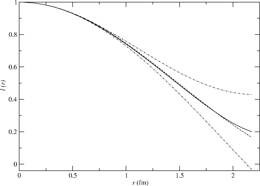
Figure 3: The Slater function $\ell_{PB}({\bf r})$ for 14 neutrons in PB. The top and bottom dash-dot lines show the $\ell_{PB}({\bf r})$ with ${\bf r}$ parallel to the 0,0,1 box side and to the 1,1,1 diagonal respectively. The middle full line shows the average $\sqrt{\overline{\ell_{PB}^{2}({\bf r})}}$, and the dashed line shows the $\ell(r)$ in the UG.

in place of the UG density matrix given by the Slater function (Eq. 14). The $\ell_{PB}$ depends upon the direction of ${\bf r}$, as illustrated in Fig. 3. The $\ell_{PB}$ is largest for ${\bf r}$ parallel to the box side and smallest along the diagonal.

The C-parts of the operators in $E(2b)$ (Eq. 11) are spherically symmetric functions of $r_{ij}$, therefore the $E(2b)$ depends only on the angle averaged value of $\ell^{2}$:

$$\overline{\ell^{2}_{PB}(r)}=\frac{1}{4\pi}\int sin\theta~{}d\theta~{}d\phi~{}\ell^{2}_{PB}({\bf r})~{},$$ (17)

at $r\leq L/2$. The $\overline{\ell^{2}_{PB}(r)}$ is fairly close to $\ell^{2}(r)$ in UG as shown in Fig. 3. Therefore the 2-body cluster contributions obtained with the UG and PB density matrices are not very different. In the variational calculations with $\Phi_{PB}$ we approximate the contributions of all $n\geq 3$-body clusters by their values in the UG. The 3-b-static cluster is calculated exactly, and the rest with chain summation approximations. We note that Fantoni and Schmidt PBFHNC have developed chain summation methods for calculations with $\Phi_{PB}$ sans tensor correlations. They retain the $\ell_{PB}$ in all the many-body cluster contributions calculated with chain summation methods.

The results of calculations with the $v6$ and $v8^{\prime}$ interactions are given in Tables 5 and 6. The values of $T_{FG}-T_{PB}$ and

$$\Delta E(2b)=E_{UG}(2b)-E_{PB}(2b)$$ (18)

are also listed in Table 6. The smallness of these differences makes the 14-neutron periodic box a good approximation for studying uniform gas $E(\rho)$. The variational parameters $\alpha$ and $\beta_{p}$ have essentially the same values in PB calculations as in UG with $d=d_{t}=L/2$. The main difference between the UG and PB energies comes from the contribution of the long range interaction, $v(r_{ij})\theta(r_{ij}-L/2)$ omitted in the PB. Its contribution denoted by $\langle v(r_{ij}>L/2)\rangle$ is estimated from UG calculations and listed in Table 6. It becomes comparable to the total $E_{UG}(\rho)$ at $\rho\sim 1.5~{}\rho_{0}$.

IV.2 Comparison with QMC Calculations

The results of the approximate VCS calculations are compared with those of QMC calculations in Tables 1 and 2 for the $v6$ and $v8^{\prime}$ interactions. Since the VMC and VCS calculations use the same wave function for the $v6$ Hamiltonian, they should ideally give the same results. The difference between them is due only to the approximations in the VCS calculations. Relative to the VMC results, the VCS total energy is higher by 8 % at $\rho_{0}/4$ and lower by 2 % at $1.5\rho_{0}$. The difference between the VCS and VMC potential energy, $\langle v6\rangle$ is similar. The clusters with $\geq 3$-neutrons give a relatively larger contribution at smaller densities (Table 5) due to the large $nn$ scattering length. It is thus not surprising that VCS has larger errors in that region. The GFMC-UC energies are below those of the VCS by 12 to 4 % in this density range. We note that the differences between the GFMC-UC and VCS or VMC potential energies are much larger, of order 20 %. This is because the present variational wave functions underestimate the correlations in matter, as is further elaborated in the next section.

In the case of the $v8^{\prime}$ Hamiltonian, the VMC calculations do not include the spin-orbit correlations while the VCS do, therefore the VMC and VCS results are not comparable in this case. However, we can compare the GFMC-UC and VCS results. As for $v6$, the GFMC-UC energies are lower by 10 % at lower densities; however, at $1.5\rho_{0}$ the VCS energy is lower by $2\pm 0.5$ MeV. Most of this difference seems to come from the spin-orbit interaction. The $\langle v_{{\bf L}\cdot{\bf S}}\rangle=-8\pm 1$ and $-12$ MeV in these two calculations at $1.5\rho_{0}$. When the density dependence of spin-orbit correlations is neglected, the leading two-neutron cluster gives a contribution proportional to $\rho^{5/3}$ to $\langle v_{{\bf L}\cdot{\bf S}}\rangle$. This comes about because the spin-orbit contributions are proportional to $\rho^{2/3}$ via the $k^{2}$ momentum dependence of $v_{{\bf L}\cdot{\bf S}}{\bf L}\cdot{\bf S}f_{{\bf L}\cdot{\bf S}}{\bf L}\cdot{\bf S}$, and the summation over particles gives an additional factor of $\rho$ for 2-body clusters. The VCS results for $\langle v_{{\bf L}\cdot{\bf S}}\rangle$ approximately follow this density dependence as shown in Table 2. Up to $\rho_{0}$ the GFMC-UC $\langle v_{{\bf L}\cdot{\bf S}}\rangle$ also has a similar density dependence. However, at $1.5\rho_{0}$ the GFMC-UC is smaller in magnitude. It could be that higher order cluster terms become more important at this density and that VCS overestimates the $v_{{\bf L}\cdot{\bf S}}$ contribution, or that, if GFMC-UC is propagated further in the imaginary time $\tau$ after the CP, the $\langle v_{{\bf L}\cdot{\bf S}}\rangle$ will decrease and the GFMC-UC energy will go down. In the present calculation we can not test this possibility because of the increase in the statistical errors due to the Fermion sign problem.

V Pair Distribution Functions

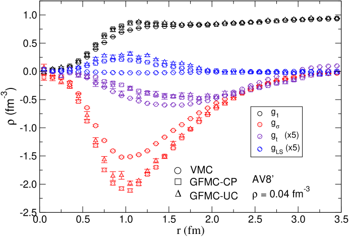
Figure 4: Pair distribution functions for the $v8^{\prime}$ interaction at rho = 0.04 fm^-3. The data sets from top to bottom correspond to central, L$\cdot$S, tensor and $\mbox{\boldmath$\sigma$}_{i}\cdot\mbox{\boldmath$\sigma$}_{j}$ pair distribution functions. Each set contains circles, squares and triangles showing the VMC, GFMC-CP and GFMC-UC results. The L$\cdot$S and the tensor distribution functions are scaled up by a factor of five.

The pair distribution functions obtained from QMC calculations with the $v8^{\prime}$ interaction are shown in Figures 4 to 7. In each figure the circles show the results of VMC calculations with a wave function containing $f6$ correlations (without L$\cdot$S correlations). Squares and triangles represent the result of the constrained path (GFMC-CP), and the unconstrained (GFMC-UC). The pair distribution functions $g_{p}(r)$ are given by the expectation value:

$$g_{p}(r)=N\sum_{i<j}\langle\Psi|\delta(r_{ij}-r)O^{p}_{ij}|\Psi\rangle,$$ (19)

with a normalization $N$ such that $g_{1}(r)\equiv g_{c}(r)$ goes to one at large distances. The $g_{2-4}$ are denoted by $g_{\sigma},g_{t}$ and $g_{LS}$ for clarity. The $g_{c}(r)$ gives the probability to find a neutron at a distance $r$ from another neutron since $O^{p=1}_{ij}=1$. In contrast $O^{p=2}_{ij}=\mbox{\boldmath$\sigma$}_{i}\cdot\mbox{\boldmath$\sigma$}_{j}$, thus $g_{\sigma}$ is proportional to the expectation value of $\delta(r_{ij}-r)\mbox{\boldmath$\sigma$}_{i}\cdot\mbox{\boldmath$\sigma$}_{j}$. Using the projection operators:

$$P_{S=0} = \frac{1}{4}(1-\mbox{\boldmath$\sigma$}_{i}\cdot\mbox{\boldmath$\sigma$}_{j})~{},$$ (20)

$$P_{S=1} = \frac{1}{4}(3+\mbox{\boldmath$\sigma$}_{i}\cdot\mbox{\boldmath$\sigma$}_{j})~{},$$ (21)

the pair distribution functions in spin $S=0$ and 1 pairs are found to be:

$$g_{S=0}(r) = \frac{1}{4}(g_{c}(r)-g_{\sigma}(r))~{},$$ (22)

$$g_{S=1}(r) = \frac{1}{4}(3g_{c}(r)+g_{\sigma}(r))~{}.$$ (23)

Since $g_{S=1}(r\rightarrow 0)\rightarrow 0$, the $g_{\sigma}(r)=-3g_{c}(r)$ at small $r$. In noninteracting Fermi gases:

$$g^{FG}_{c}(r) = 1-\frac{1}{2}\ell^{2}(r)~{},$$ (24)

$$g^{FG}_{\sigma}(r) = -\frac{3}{2}\ell^{2}(r)~{},$$ (25)

$$g^{FG}_{t}(r) = g^{FG}_{LS}=0~{}.$$ (26)

The VMC calculations do not have spin-orbit correlations, and give $g_{LS}\sim 0$.

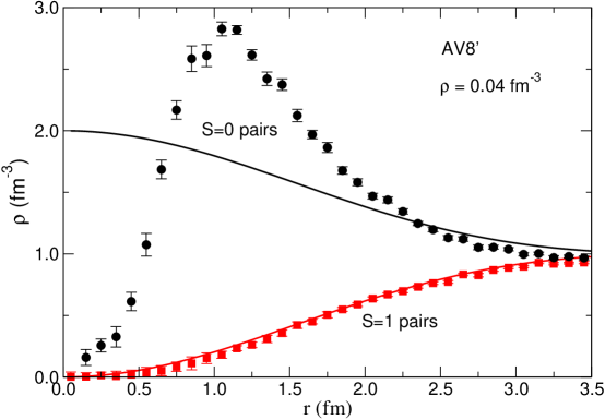
Figure 8: Pair distribution functions for spin 0 and spin 1 pairs at $\rho=0.04$ fm^-3; results of unconstrained GFMC calculations are compared to distributions in noninteracting FG shown by solid lines.

At $\rho=0.04$ fm^-3, there is a very strong pairing into spin 0 states as indicated by the large negative $g_{\sigma}$. It can be seen more clearly in Figure 8 which compares the $g_{S=0,1}(r)$ in neutron matter and Fermi gases. The large peak of the $g_{S=0}$ is due to the large negative $nn$ scattering length; it should be relatively model independent and grow at smaller densities. This pairing is present in the variational calculations, though underestimated by $\sim$ 25 %. The tensor and $L\cdot S$ correlations are quite modest at these low densities. There is little change between the constrained GFMC-CP and unconstrained GFMC-UC, indicating reasonably good convergence within this class of wave functions. The tensor correlations are long-ranged, extending nearly to the $L/2$ limit imposed by the periodic boundary conditions. This same behavior is seen even when starting the GFMC with trial wave functions having much shorter range correlations.

The correlations at $\rho=0.08$ fm^-3 are fairly similar, though the spin correlation is not as large, and the tensor and $L\cdot S$ correlations are becoming more significant. The $g_{LS}$ is essentially zero in the variational calculation, and underestimated in CP GFMC.

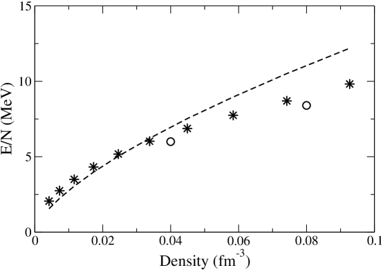
Figure 9: The energy of neutron matter at low densities. The stars give the results of Ref.FP81 and the circles of the present calculation. The dashed line shows $0.5~{}E_{FG}$.

At the largest densities considered, $\rho$ = 0.16 and 0.24 fm^-3, the differences between the variational, GFMC-CP, and the GFMC-UC results are quite large. Both the tensor and $L\cdot S$ correlations are quite important and significantly underestimated in the VMC and GFMC-CP calculations. We see a transition from low densities, where the S-wave interaction and spin zero pairing is dominant, to these higher densities, where the P-wave interactions are crucial. It could be associated with the ³P₂-³F₂ pairing BCLL92 expected at higher densities. In VCS calculations with three nucleon interaction (see Fig.9 of Ref.AP97 ) such a behavior is associated with the onset of pion condensation.

VI Density Dependence of Neutron Matter Energy

The total energy of neutron matter interacting with the $v8^{\prime}$ potential is reported in Table 7. It is obtained by adding the box corrections listed in Table 6 to the GFMC-UC energies listed in Table 2. The ratio of neutron matter $E(\rho)$ to the noninteracting neutron Fermi gas energy is also listed in Table 7. This ratio approaches $\sim 0.5$ at low densities.

The properties of low density neutron matter are dominated by the large negative $nn$ scattering length. When $|ak_{F}|<<1$ we have the well known low density expansion FWbook :

$$E(\rho)=E_{FG}(\rho)\left[1+\frac{10}{9\pi}ak_{F}+\frac{4}{21\pi^{2}}(11-2ln2)(ak_{F})^{2}+...\right]~{}.$$ (27)

Such an expansion is not useful for neutron matter because even at densities as low as 1% of $\rho_{0}$, $|ak_{F}|>6$. The limit $ak_{F}\rightarrow-\infty$ is perhaps more applicable to neutron gas than the low density expansion, as suggested by Bertsch Bertsch . In this limit it is known that:

$$E(\rho)=E_{FG}(\rho)\xi~{}.$$ (28)

The estimates of $\xi$ range from 0.326 baker ; hh to 0.568 baker to 0.59 ERS97 . Recent quantum Monte Carlo calculations dfg give $\xi\sim 0.54$ for the normal phase and $\xi=0.44\pm 0.02$ for the superfluid phase. Most many-body calculations, both Brueckner and variational, give $\xi\sim 0.5$ for normal neutron matter. As an example, we compare the energies of neutron matter calculated with the CSM in 1981 FP81 with the $E_{FG}$ and results of present calculation in Figure 9.

Eq. 28 implies that at low densities the interaction energy of neutron matter becomes proportional to $k_{F}^{2}$ as is the FG kinetic energy. This interaction energy is proportional to density $(=k_{F}^{3}/3\pi^{2})$ times the volume integral of the effective $G$-interaction, related to the bare $v$-interaction by the well-known Brueckner equation $G\phi=v\psi$. Here $\phi$ and $\psi$ are the unperturbed and perturbed two-nucleon wave functions. At small relative momenta of interest at low-densities, $\phi=1$, and in vacuum $\psi=1-a/r$ beyond the the range $R_{v}$ of $v$. When $-a/R_{v}>>1$, as is the case for neutrons, we can neglect the $1$ in comparison and approximate the $\psi$ by $-a/R_{v}$. The effective interaction in vacuum is essentially enhanced by a factor $-a/R_{v}$ by the large scattering length. In matter the effective scattering length is limited by the interparticle spacing of order $1/k_{F}$. Thus, when $-ak_{F}>>1$, the $G$ is enhanced by a factor proportional to $1/k_{F}R_{v}$, its integral becomes proportional to $1/k_{F}$, and the interaction energy proportional to $k_{F}^{2}$. At higher densities we see a deviation from Eq. 28 in Fig. 9. It starts when $k_{F}R_{v}$ becomes of order 1 and the first (unit) term of $\psi$ can not be neglected. When $R_{v}\rightarrow 0$, as in the challenge problem proposed by Bertsch, Eq. 28 is valid at all densities when $a=-\infty$.

Most of the nonrelativistic Skyrme as well as the relativistic mean field energy density functions commonly used to study nuclei and neutron star matter assume that $\xi=1$. None of these therefore can reproduce the equation of state, $E_{0}(\rho)$ of pure neutron matter PR95 obtained from realistic interactions even at low densities. The effective interaction used in mean field models must diverge as $\rho\rightarrow 0$ due to large $nn$ scattering length. Energy density functionals containing such low-density divergences PRlect are probably necessary to study nuclei near neutron drip line or in the inner crust of neutron stars.

VII Superfluidity and Accuracy of the Present Calculations

Quantum Monte Carlo calculations of 14 neutrons described above start from a correlated Slater trial wave function. This trial function is appropriate for the normal phase of Fermi liquids and is used here as the starting point for the CP GFMC and to obtain the constraints used to limit the Fermion sign problem in that calculations. Its results are expected to give the equation of state of the normal phase. The long-wavelength properties of the correlated Slater wave function do not include the expected superfluid properties of neutron matter. Generally, the energy of the superfluid phase is not significantly different from that of the normal one, since in most systems the pairing is confined near the Fermi surface, and involves only relatively few particles. Here, however, the magnitude of the $nn$ scattering length is very large compared to the interparticle spacing, the pairing is exceptionally strong, and affects all the particles.

In principle it may be possible for the unconstrained GFMC calculations to relax to the lower energy superfluid phase provided there is sufficient overlap between the fourteen particle wavefunctions of these phases. However, the unconstrained calculations are limited to fairly short paths, due to small unconstrained propogation time, and hence are unlikely to relax to the superfluid phase. In calculations with simple spin-independent, short-range interactions with $a=-\infty$, Schmidt et al. dfg find, upon including superfluid pairing into the trial wave function, important effects, including an $\approx$ 20% reduction in the energy per particle mentioned in the previous section.

One of the important features of the Monte Carlo approach pursued here is that it can be extended to include BCS pairing into the trial wave function. Thus it will be possible to study properties of superfluid neutron matter with realistic models of the $nn$ interaction. We are presently pursuing such studies. The main remaining uncertainty in the equation of state of low density neutron matter is probably due to the neglected difference in the $E_{0}(\rho)$ of normal and superfluid phases.

VIII Acknowledgments

We would like to thank K. E. Schmidt for valuable discussions. The work of J.C. is supported by the U.S. Department of Energy under contract W-7405-ENG-36, while that of J.M., V.R.P. and D.G.R. is partly supported by the US National Science Foundation grant PHY00-98353. The QMC calculations reported here were performed at the National Energy Research Supercomputer facility.

Appendix A Elementary four-body circular exchange diagrams

The 4-body diagrams in the expansion of $E_{V}-T_{FG}$ (Eq. 10), not included in the Fermi hypernetted chain summation, are called elementary PW79 . In Fermi liquids they were first calculated by Zabolitzky zab81 . The circular exchange diagram shown in Fig. 10 is the only one of first order in the expansion in powers of $(F^{2}_{ij}-1)$, among these. It therefore has special importance as emphasized by Krotscheck krot79 , and was included in the study of nuclear matter structure functions npa473 . The thick interaction line in this diagram represents:

$$I_{13}=F_{13}\left(v_{13}F_{13}-\frac{\hbar^{2}}{m}[\nabla^{2}F_{13}]\right)~{}.$$ (29)

We approximate the contribution of this diagram with:

$$\frac{\rho^{3}}{4} \int d^{3}r_{12}d^{3}r_{13}d^{3}r_{14}\ell_{12}\ell_{23}\ell_{34}\ell_{41}f_{c}^{2}(r_{12})f_{c}^{2}(r_{23})f_{c}^{2}(r_{34})f_{c}^{2}(r_{41})$$ (30)

$$C \left[(e_{12}e_{23}e_{34}+e_{34}e_{23}e_{12})I_{13}(F^{2}_{24}-1)\right]~{}.$$

The term with $e_{34}e_{23}e_{12}$ takes into account the circular exchange in the other direction. The spin-orbit interactions and correlations, and the spin correlations between neutron pairs 12, 23, 34 and 41 are neglected in this approximation expected to have an accuracy of order 20 %.

Table 1: Quantum Monte Carlo and VCS results for 14 neutrons in PB with the $v6$ Hamiltonian (MeV per neutron). Statistical errors are indicated in parenthesis.

Method	$\rho$ (fm${}^{-3})$	0.04	0.08	0.16	0.24
VMC	$~{}~{}~{}\langle H\rangle$	7.04(01)	11.32(01)	21.39(01)	34.30(01)
GFMC-CP		6.72(01)	10.64(01)	19.80(02)	31.90(02)
GFMC-UC		6.75(01)	10.64(03)	19.91(11)	32.15(08)
VCS		7.6	11.9	21.2	33.6
VMC	$~{}~{}~{}\langle v6\rangle$	$-$9.92(03)	$-$16.17(05)	$-$22.79(08)	$-$26.10(11)
GFMC-CP		$-$11.75(08)	$-$18.64(09)	$-$28.01(08)	$-$32.94(25)
GFMC-UC		$-$11.36(13)	$-$18.17(36)	$-$26.62(71)	$-$32.71(71)
VCS		$-$9.2	$-$15.4	$-22.7$	$-$26.6

Table 2: Quantum Monte Carlo and VCS results for 14 neutrons in PB with the $v8^{\prime}$ Hamiltonian (MeV per neutron).

Method	$\rho$ (fm${}^{-3})$	0.04	0.08	0.16	0.24
VMC	$~{}~{}~{}\langle H\rangle$	7.16(01)	11.678(07)	21.82(12)	35.02(01)
GFMC-CP		6.43(01)	10.02(02)	18.54(04)	30.04(04)
GFMC-UC		6.32(03)	9.501(06)	17.00(27)	28.35(50)
VCS		7.0	10.3	17.4	26.3
VMC	$~{}~{}~{}\langle v6\rangle$	$-$9.74(03)	$-$15.72(6)	$-$21.64(09)	$-$24.37(11)
GFMC-CP		$-$11.85(09)	$-$18.34(11)	$-$27.72(15)	$-$32.34(23)
GFMC-UC		$-$11.44(19)	$-$17.83(30)	$-$25.62(87)	$-$30.52(1.35)
VCS		$-$9.3	$-$15.1	$-$21.6	$-$24.9
VMC	$~{}~{}~{}\langle v_{{\bf L}\cdot{\bf S}}\rangle$	0.07(01)	0.26(01)	0.13(01)	0.21(01)
GFMC-CP		$-$0.23(11)	$-$1.37(03)	$-$2.69(03)	$-$4.08(08)
GFMC-UC		$-$0.85(04)	$-$2.59(15)	$-$6.24(50)	$-$7.98(98)
VCS		$-$0.88	$-$2.3	$-$6.9	$-$12.1
$-6.9(\rho/\rho_{0})^{5/3}$		$-$0.68	$-$2.2	$-$6.9	$-$13.6

Table 3: Results of VCS calculations of the UG $E(\rho)$ (MeV per neutron) with optimum $d$ and $d_{t}$, in MeV. Contributions with an * are estimated using chain summation approximation; those without are calculated exactly. The bottom two rows give the approximate 3-b-static*, for comparison with the exact 3-b-static, and 4-b-elementary* circular exchange contribution included in $\geq 4$-b-static*

$\rho$ (fm-3)	0.04	0.08	0.16	0.24
$d$ (fm)	3.66	3.31	2.29	2.20
$d_{t}$ (fm)	6.17	5.56	5.22	4.69
$\alpha$	0.89	0.87	0.80	0.72
$\beta_{\sigma}$	0.8	0.8	1.0	1.0
$\beta_{t}$	0.9	1.0	0.9	0.9
$\beta_{b}$	0.9	0.8	1.0	1.1
$T_{FG}$	13.9	22.1	35.1	46.0
2-b-Total	$-$10.1	$-$16.9	$-$25.5	$-$33.9
3-b-static	4.9	6.9	3.7	3.5
$\geq$ 4-b-static*	$-$2.3	$-$3.1	$-$ 1.5	$-$ 1.1
$\geq 3$-b-${\bf L}\cdot{\bf S}$*	0.1	0.2	0.2	$-$ 0.1
Total $E(\rho)$	6.6	9.2	12.0	14.5
3-b-static*	4.6	6.6	3.5	3.2
4-b-elementary*	$-$ 0.5	$-$0.5	0.5	0.7

Table 4: Results of VCS calculations of the UG $E(\rho)$ (MeV per neutron) with $d=d_{t}=L/2$, in MeV. Contributions with an * are estimated using chain summation approximation; those without are calculated exactly.

$\rho$ (fm-3)	0.04	0.08	0.16	0.24
$L/2$ (fm)	3.52	2.80	2.22	1.94
$\alpha$	0.90	0.85	0.80	0.80
$\beta_{\sigma}$	0.80	0.9	0.9	1.0
$\beta_{t}$	1.50	2.0	1.0	1.0
$\beta_{b}$	0.85	0.9	1.1	1.1
$T_{FG}$	13.9	22.1	35.1	46.0
2-b-Total	$-$ 9.7	$-$14.9	$-$23.0	$-$29.9
3-b-static	3.9	2.7	$-$0.1	$-$0.8
$\geq$ 4-b-static*	$-$1.5	$-$0.7	$-$ 0.0	$-$ 0.0
$\geq 3$-b-${\bf L}\cdot{\bf S}$*	0.0	0.0	0.2	$-$ 0.4
Total $E(\rho)$	6.7	9.2	12.1	14.8

Table 5: Results of PB variational calculations with $v6$ interaction truncated at $r=L/2$. The variational parameters are listed in Table 4, and the energies are MeV per neutron.

$\rho$ (fm-3)	0.04	0.08	0.16	0.24
$T_{PB}$	14.1	22.4	35.6	46.6
2-b-Total	$-$9.0	$-$12.6	$-$14.2	$-$12.3
$\geq$3-b-Total	2.5	2.0	$-$0.1	$-$0.7
Total $E(\rho)$	7.6	11.9	21.2	33.6

Table 6: Results of PB variational calculations with $v8^{\prime}$ interaction truncated at $r=L/2$. The variational parameters are listed in Table 4, and the last three rows give the differences between PB and UG contributions. All energies are in MeV per neutron.

$\rho$ (fm-3)	0.04	0.08	0.16	0.24
$T_{PB}$	14.1	22.4	35.6	46.6
2-b-Total	$-$9.5	$-$14.0	$-$18.3	$-$19.1
$\geq$3-b-Total	2.4	1.9	0.1	$-$1.2
Total $E(\rho)$	7.0	10.3	17.4	26.3
$T_{FG}-T_{PB}$	-0.2	-0.3	-0.5	-0.7
$\Delta E(2b)$	-0.0	-0.1	-0.1	-0.1
$\langle v(r_{ij}>L/2)\rangle$	$-$0.1	$-$0.8	$-$4.5	$-$10.7

Table 7: Neutron matter energy with the $v8^{\prime}$ interaction in MeV per neutron.

$\rho$ (fm-3)	0.04	0.08	0.16	0.24
GFMC-UC	6.3	9.5	17.0	28.4
Box Correction	$-$0.3	$-$1.1	$-$5.1	$-$11.5
Total $E(\rho)$	6.0	8.4	12.1	16.9
$E(\rho)/E_{FG}(\rho)$	0.43	0.38	0.34	0.37

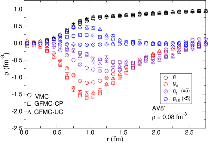
Figure 5: Pair distribution functions for the $v8^{\prime}$ interaction at rho = 0.08 fm^-3, as in Figure 4.

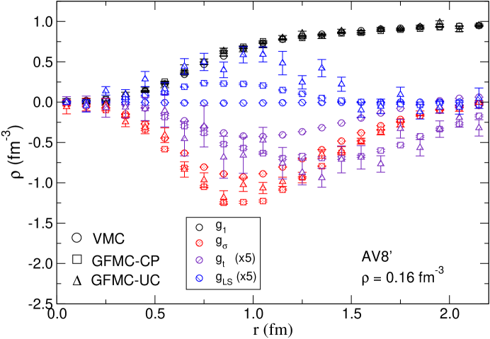
Figure 6: Pair distribution functions for the $v8^{\prime}$ interaction at rho = 0.16 fm^-3, as in Figure 4.

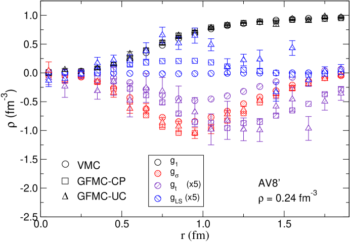
Figure 7: Pair distribution functions for the $v8^{\prime}$ interaction at rho = 0.24 fm^-3, as in Figure 4.

Figure 10: The lowest order elementary 4-body circular exchange diagram. The dashed line shows $F_{24}^{2}-1$, the thick solid line denotes the interaction link, and the thin lines with direction show the exchange pattern.

References

- (1) C. J. Pethick and D. G. Ravenhall, Annu. Rev. Nucl. Part. Sci. 45, 429 (1995).
- (2) H. Heiselberg and V. R. Pandharipande, Annu. Rev. Nucl. Part. Sci. 50, 481 (2000).
- (3) W. Nazarewicz in The RIA White paper, www.nscl.msu.edu/future/ria/process/ whitepapers/durham2000.pdf (2000).
- (4) L. Engvik, M. Hjorth-Jensen, R. Machleidt, H. Müther and A. Polls, Nucl. Phys. A627, 85 (1997); L. Engvik, The nuclear equation of state, Thesis, Univ. of Oslo (1999).
- (5) M. Baldo, I. Bombaci and G. F. Burgio, Astron. Astrophys. 328, 274 (1997).
- (6) R. B. Wiringa, V. Fiks and A. Fabrocini, Phys. Rev. C 38, 1010 (1988).
- (7) A. Akmal, V. R. Pandharipande and D. G. Ravenhall, Phys. Rev. C 58, 1804 (1998).
- (8) H. Q. Song, M. Baldo, G. Giansiracusa and U. Lombardo, Phys. Rev. Lett. 81, 1584 (1998).
- (9) J. Morales, V. R. Pandharipande and D. G. Ravenhall, Phys. Rev. C 66, 054308 (2002).
- (10) R. B. Wiringa, S. C. Pieper, J. Carlson and V. R. Pandharipande, Phys. Rev. C 62, 014001 (2000).
- (11) S. C. Pieper, K. Verga and R. B. Wiringa, Phys. Rev. C 66, 044310 (2002).
- (12) S. C. Pieper, V. R. Pandharipande, R. B. Wiringa and J. Carlson, Phys. Rev. C 64, 014001 (2001).
- (13) K. E. Schmidt and S. Fantoni, Phys. Lett. B446, 99 (1999).
- (14) S. Fantoni, A. Sarsa and K.E. Schmidt, Phys Rev Lett 87, 181101 (2001).
- (15) G. F. Bertsch, Challenge Problem in Many-Body Physics www.phys.washington.edu / mbx/george (1998)
- (16) J. R. Engelbrecht and M. Randeria and C.A.R. Sá de Melo, Phys. Rev. B 55, 15153 (1997).
- (17) J. Carlson, V. R. Pandharipande, K. E. Schmidt and S-Y Chang, private comunication (2002).
- (18) B. S. Pudliner, V. R. Pandharipande, J. Carlson, S. C. Pieper and R. B. Wiringa, Phys. Rev. C 56, 1720 (1997).
- (19) D. M. Ceperley, Rev. Mod. Phys. 67, 279 (1995).
- (20) G. Ortiz and P. Ballone, Phys. Rev. B 50, (1994).
- (21) J. B. Anderson, J. Chem. Phys. 63, 1499 (1975).
- (22) Shiwei Zhang, J. Carlson, and J. E. Gubernatis, Phys. Rev. B55 , 7464 (1997); J. Carlson, J. E. Gubernatis, G. Ortiz, and Shiwei Zhang, Phys. Rev. B59, 12788 (1999).
- (23) V. R. Pandharipande and R. B. Wiringa, Rev. Mod. Phys. 51, 821 (1979).
- (24) S. Fantoni and K. E. Schmidt, Nucl. Phys. A690, 456, 2001.
- (25) M. Baldo, J. Cugnon, A. Lejeune and U. Lombardo, Nucl. Phys. A536, 349 (1992).
- (26) A. Akmal and V. R. Pandharipande, Phys. Rev. C 56, 2261 (1997).
- (27) A. L. Fetter and J. D. Walecka, Quantum Theory of Many Particle Systems, McGraw-Hill (1971).
- (28) G. A. Baker, Phys. Rev. C 60, 054311 (1999).
- (29) H. Heiselberg, Phys. Rev. A 63, 043606 (2001).
- (30) B. Friedman and V. R. Pandharipande, Nucl. Phys. A361, 501 (1981).
- (31) V. R. Pandharipande and D. G. Ravenhall, in Proc. NATO Advanced Research Workshop on Nuclear Matter and Heavy Ion Collisions, Les Houches, Ed. M. Soyeur et.al., pp 103 Plenum (1989).
- (32) J. G. Zabolitzky, Adv. Nucl. Phys. 12, 1 (1981).
- (33) E. Krotscheck, Nucl. Phys. A317, 149 (1979).
- (34) R. Schiavilla, D. S. Lewart, V. R. Pandharipande, S. C. Pieper, R. B. Wiringa and S. Fantoni, Nucl. Phys. A473, 267 (1987).