Off-shell pairing correlations from meson-exchange theory of nuclear forces

Abstract

We develop a model of off-mass-shell pairing correlations in nuclear systems, which is based on the meson-exchange picture of nuclear interactions. The temporal retardations in the model are generated by the Fock exchange diagrams. The kernel of the complex gap equation for baryons is related to the in-medium spectral function of mesons, which is evaluated nonperturbatively in the random phase approximation. The model is applied to the low-density neutron matter in neutron star crusts by separating the interaction into a long-range one-pion-exchange component and a short-range component parametrized in terms of Landau Fermi liquid parameters. The resulting Eliashberg-type coupled nonlinear integral equations are solved by an iterative procedure. We find that the self-energies extend to off-shell energies of the order of several tens of MeV. At low energies the damping of the neutron pair correlations due to the coupling to the pionic modes is small, but becomes increasingly important as the energy is increased. We discuss an improved quasiclassical approximation under which the numerical solutions are obtained.

I Introduction

The lowest order in the interaction mean-field treatments of the nuclear pairing in bulk nuclear matter and in finite nuclei are conceptually simple and have been reasonably consistent with the phenomenology of these systems. The Hartree-Fock-Bogolyubov (HFB) theory with zero- or finite-range (e.g., the Skyrme and the Gogny) phenomenological forces has been the standard tool in the studies of the nuclear structure to describe the bulk of the experimental data RING_SCHUCK . At the same time, the calculations of the pairing gaps in bulk nuclear matter based on the Bardeen-Cooper-Schrieffer (BCS) theory with interactions modeled by the bare (realistic) nucleon-nucleon forces and quasiparticle spectra in the effective mass approximation are not inconsistent with the cooling simulations of neutron stars or the phenomenology of their rotation dynamics. Although there is no direct evidence for higher order correlations in the phenomenology of nuclear systems, these cannot be discarded on the basis of purely phenomenological arguments. The effective forces used in the HFB calculations are fitted to the pairing properties of (some) nuclei, consequently the contributions beyond mean field are built-in automatically (e.g., the effective Skyrme or Gogny forces include the contributions from the ladder diagrams). The values of the pairing gaps deduced from the phenomenology of neutron stars depend sensitively on the physical input, such as the equation of state, the matter composition, and its dynamical properties. Provided the uncertainties in these ingredients the phenomenological values of the gap can be off by an order of magnitude. From the theory point of view the higher order correlations might not be manifest due to large cancellation between the vertex and propagator renormalization.

The on-mass-shell properties of the pairing gaps are well understood at the mean-field level. Upon ignoring the renormalization effects, the on-mass-shell gaps can be directly computed from the nucleon-nucleon scattering phase shifts. Since the pairing is a low-temperature phenomenon, a well-defined Fermi sea implies that the on-shell self-energies of weakly excited quasiparticles can be expanded around their Fermi momentum. The magnitude of the gap is then controlled by the renormalization of density of states at the Fermi surface. Since the ratio of the momentum-dependent effective mass to the bare mass is less than unity the reduction of the density of states causes a reduction of the pairing gap.

The early work to construct renormalization schemes for strongly interacting fermions introduced wave-function renormalization factors in the kernel of the gap equation and modeled the pairing interaction in terms of particle-hole irreducible vertices MIGDAL . These were related to the phenomenological Landau Fermi liquid parameters which can (in principle) be fixed by comparison with experiments. The Landau parameters can be obtained from ab initio microscopic calculations as well, which are needed, for example, to describe isospin asymmetric nuclear systems that are not directly accessible in laboratories Backman:sx ; Dickhoff:qr ; Dickhoff:qr2 ; Dickhoff:qr3 . Various aspects of the pairing in the infinite nuclear matter beyond the mean-field (BCS) approximation were addressed during the past two decades by employing either more advanced schemes to calculated the self-energy and vertex corrections and/or modern (phase-shift equivalent) interactions. This work includes the microscopic calculations of the effective interactions and Landau parameters using variants of the Babu-Brown BABU_BROWN or related (e.g., polarization potential) schemes of summing the polarization graphs in neutron matter WAMBACH1 ; WAMBACH2 ; SCHULZE . The polarization effects were found to suppress the on-shell pairing gaps by large factors. Earlier, similar reduction was found from the correlated basis variational calculations based on the Jastrow ansatz for fermionic wave functions CLARK1 ; CLARK2 ; CLARK3 . More recent work concentrated on the calculations of the wave-function renormalizations and their implementations in gap equations employing self-energies derived within Brueckner theory at first BALDO and second LOMBARDO order in the hole-line expansion. While again a suppression was found due to the wave function renormalizations, supplementing these self-energy corrections with appropriate vertex corrections largely compensates for the latter effect SHEN . The finite temperature $T$ matrix was utilized to deduce the pairing correlations that include full spectral information on the system by using the Thouless criterion ROEPKE , wave-function renormalizations in the gap equations, or the $T$ matrix in the superfluid phase BOZEK . The reduction of the critical temperature of superfluid phase transition found in these approaches is due to dressing of propagators in the particle-particle channel, i.e., the analog effect of the self-energy renormalizations in the Brueckner scheme BALDO ; LOMBARDO . (It is unrelated to the reduction mentioned above caused by the polarization of the interaction that follows from the resummations in the particle-hole channels.) Renormalization group approach has been used to resume the particle-hole channels and deduce the pairing gap from the matrix elements defined on the Fermi surface RENORM1 ; the overall magnitude of the reduction of the gap is consistent with the results mentioned above. The pairing gaps computed from the renormalization group motivated interactions are in good agreement with the calculations based on the original bare interactions RENORM2 or the effective Gogny interactions RENORM3 below the renormalization scale.

The off-mass-shell physics of the nuclear pairing is much less understood. Contributions to the (complex) pairing gap can be generated by time nonlocal interactions. The simplest example is the fermionic Fock-exchange diagram in a boson-exchange interaction model. The generic theory of the boson-exchange superconductors is known in the form first developed by Eliashberg ELIASHBERG to describe the superconductivity in materials where the electron-phonon coupling is of the order of unity (see also the general references SCHRIEFFER ; SCALAPINO ; MAHAN ). Because the theory contains another small parameter - the ratio of the phonon Debye energy to the Fermi energy of electrons - the vertex corrections (according to the Migdal theorem) can be neglected. For the same reason, the quasiclassical approximation can be used where the on-shell energy of the original Green’s functions are integrated out. In our context the coupling of the pionic modes to baryons is not small and the characteristic energies of the off-shell excitations are not small compared to the Fermi energy. Below, we shall partially overcome these difficulties, first, by including a vertex renormalization by the short-range correlations in the pion-nucleon vertex and, second, by applying an improved version of the quasiclassical approximation.

Pairing in nuclear systems, induced by retarded interactions, was discussed previously in Refs. SEDRAKIAN ; TERASAKI ; KAMERDZHIEV . In the context of laboratory nuclei the retarded pairing interaction is driven by an exchange of virtual phonons - low-lying collective bosonic excitation TERASAKI ; KAMERDZHIEV . In the astrophysical context of neutron star crusts the attractive pairing interaction is mediated by an exchange of real phonons of the nuclear Coulomb lattice of the crusts SEDRAKIAN . The approach taken here differs from the models above in the nature of the bosonic modes that mediate the pairing interactions. While the density fluctuations are responsible for the pairing interaction in the models above, we concentrate here at the modes that have the quantum numbers of pions.

In what follows, we construct a model of pairing in neutron matter that is based on the meson-exchange picture of the nuclear interactions. Specific to our model is the explicit treatment of the mesonic degrees of freedom including retardation. Unlike the potential models, the interaction incorporates medium modifications of the dispersion relation of the mesons (pions) and they are treated dynamically, i.e., only in the static limit the retarded interaction reduces to a meson (pion)-exchange potential. We note that the meson-exchange picture of pairing is known from applications of the Walecka mean-field model to the pairing problem RMF1 ; RMF2 ; RMF3 . These approaches, however, do not include the pion dynamics or retardation. In computing the renormalization of the pionic propagator and the pion-nucleon vertex, we shall use a simplified version of the resummation of the particle-hole diagrams by modeling the residual interaction in terms of a contact approximation to the $g^{\prime}$ Landau parameter. This corresponds to the random phase approximation (RPA) renormalizations of pion propagators in Migdal’s theory of finite Fermi systems MIGDAL2 . The retardation effects are included by evaluating the Fock (exchange) self-energies of neutrons which are coupled to dynamical (off-mass-shell) pions. We determine numerically the resulting off-mass-shell gap function and wave-function renormalization self-consistently by solving the coupled integral equations for these two complex functions.

To elucidate our model, we start with the $\pi_{0}$-exchange interaction among neutrons in a low -density neutron matter relevant for the physics of neutron star crusts. In the density regime $(0.002-0.5)~{}\rho_{0}$, where $\rho_{0}=0.17$ fm^-3 is the nuclear saturation density, the matter in neutron stars is an admixture of unbound neutron liquid and a Coulomb lattice of nuclei with a charge-neutralizing background of relativistic electrons BBP ; NV ; HAENSEL . We shall assume that the neutrons form a homogenous Fermi liquid which is characterized by an isotropic Fermi surface.

The remainder of the paper is organized as follows. Section. II is devoted to the formulation of the model in the framework of the real time Green’s functions formalism. Section. III describes a method of solution of the coupled, nonlinear integral Eliashberg equations. The results are discussed for the case under study – the pairing in the low-density neutron matter – where the retarded pairing interaction is mediated by an exchange of neutral pions. Section. IV contains our conclusions. In the Appendix we discuss the quasiclassical approximation to the propagators and its improved version, which is used in our numerical work.

II Model

We shall formulate the model in terms of the real-time contour-ordered Green’s functions KELDYSH . The imaginary time Matsubara formalism is well suited for our purposes, since we assume the system to be in equilibrium, however, the numerical solution of the equations formulated on the real frequency axis are technically simpler compared to the solution of the imaginary time equations. The latter require a summation of finite number of discrete Matsubara frequencies with a certain cutoff frequency which is followed by an analytical continuation to the real axis; the former are solved directly on the real axis.

The real-time treatment of a superfluid system requires a $4\times 4$ matrix of propagators and self-energies in general KELDYSH . A $2\times 2$ structure is needed to account for the anomalous correlations due to the pairing. The elements of the Nambu-Gor’kov matrix propagator $\underline{G}_{\alpha\beta}(x,x^{\prime})$ are defined as

$$\left(\begin{array}[]{cc}G_{\alpha\beta}(x,x^{\prime})&F_{\alpha\beta}(x,x^{\prime})\\ -F^{\dagger}_{\alpha\beta}(x,x^{\prime})&\overline{G}_{\alpha\beta}(x,x^{\prime})\\ \end{array}\right)=\left(\begin{array}[]{cc}-i\langle T\psi_{\alpha}(x)\psi_{\beta}^{\dagger}(x^{\prime})\rangle&\langle\psi_{\alpha}(x)\psi_{\beta}(x^{\prime})\rangle\\ \langle\psi_{\alpha}^{\dagger}(x)\psi_{\beta}^{\dagger}(x^{\prime})\rangle&-i\langle\tilde{T}\psi_{\alpha}(x)\psi_{\beta}^{\dagger}(x^{\prime})\rangle\\ \end{array}\right),$$ (5)

where $\psi_{\alpha}(x)$ are the baryon field operators, $x$ is the space-time coordinate, $\alpha$ and $\beta$ stand for the internal (discrete) degrees of freedom, $T$ and $\tilde{T}$ are the symbols for time ordering and inverse time ordering of operators, respectively. Each of the propagators above can be viewed as a $2\times 2$ matrix in the Keldysh space, if we map the time structure of the propagators on a real-time contour. For example, the elements of the normal propagator in the Keldysh space, ${\underline{\hat{G}}}_{\alpha\beta}(x,x^{\prime})$ (the hat hereafter indicates that the propagator is contour ordered) are defined as

$$\left(\begin{array}[]{cc}\underline{G}^{c}_{\alpha\beta}(x,x^{\prime})&\underline{G}^{<}_{\alpha\beta}(x,x^{\prime})\\ \underline{G}^{>}_{\alpha\beta}(x,x^{\prime})&\underline{G}^{a}_{\alpha\beta}(x,x^{\prime})\\ \end{array}\right)=\left(\begin{array}[]{cc}-i\langle T\psi_{\alpha}(x)\psi_{\beta}^{\dagger}(x^{\prime})\rangle&i\langle\psi_{\alpha}^{\dagger}(x^{\prime})\psi_{\beta}(x)\rangle\\ -i\langle\psi_{\alpha}(x)\psi_{\beta}^{\dagger}(x^{\prime})\rangle&-i\langle\tilde{T}\psi_{\alpha}(x)\psi_{\beta}^{\dagger}(x^{\prime})\rangle\\ \end{array}\right).$$ (10)

The off-diagonal elements of the matrix (10) have their time arguments on the opposite branches of the time contour, while the upper (lower) diagonal elements have their both time arguments on the positive (negative) branch of the contour (hence the time-ordering symbols; see for details Ref. KELDYSH ). The remainder propagators are defined in a similar way. We note that even in the non-equilibrium theory only a limited subset of the elements of the matrices above carry new information. The Keldysh structure will be used below as a convenient tool for writing down the finite temperature expressions for diagrams. Eventually, we will find that the final expressions can be written only in terms of the normal and anomalous retarded propagators.

The $4\times 4$ matrix Green’s function satisfies the familiar Dyson equation

$$\underline{\hat{G}}_{\alpha\beta}(x,x^{\prime})=\underline{\hat{G}}^{0}_{\alpha\beta}(x,x^{\prime})+\sum_{\gamma,\delta}\int\!\!d^{4}x^{\prime\prime}d^{4}x^{\prime\prime\prime}\underline{\hat{G}}^{0}_{\alpha\gamma}(x,x^{\prime\prime\prime})\underline{\hat{\Sigma}}_{\gamma\delta}(x^{\prime\prime\prime},x^{\prime\prime})\underline{\hat{G}}_{\delta\beta}(x^{\prime\prime},x^{\prime}),$$ (11)

where the free-propagator matrices are diagonal in both spaces and the matrix structure of the self-energies is identical to that of the propagators (see for details Ref. KELDYSH ). Fourier transforming Eq. (11) with respect to the relative coordinate $x=x-x^{\prime}$ one obtains the Dyson equation in the momentum representation; in this representation the components of the Nambu-Gor’kov matrix obey the following coupled Dyson equations

$$\hat{G}_{\alpha\beta}(p) = \hat{G}_{0\alpha\beta}(p)+\hat{G}_{0\alpha\gamma}(p)\left[\hat{\Sigma}_{\gamma\delta}(p)\hat{G}_{\delta\beta}(p)+\hat{\Delta}_{\gamma\delta}(p)\hat{F}^{\dagger}_{\delta\beta}(p)\right],$$ (12)

$$\hat{F}^{\dagger}_{\alpha\beta}(p) = \hat{G}_{0\alpha\gamma}(-p)\left[\hat{\Delta}^{\dagger}_{\gamma\delta}(p)\hat{G}_{\delta\beta}(p)+\hat{\Sigma}_{\gamma\delta}(-p)\hat{F}^{\dagger}_{\delta\beta}(p)\right],$$ (13)

$$\hat{F}_{\alpha\beta}(p) = \hat{G}_{0\alpha\gamma}(p)\left[\hat{\Delta}_{\gamma\delta}(p)\hat{G}_{\delta\beta}(-p)+\hat{\Sigma}_{\gamma\delta}(p)\hat{F}_{\delta\beta}(p)\right],$$ (14)

$$\hat{G}_{\alpha\beta}(-p) = \hat{G}_{0\alpha\beta}(-p)+\hat{G}_{0\alpha\gamma}(-p)\left[\hat{\Sigma}_{\gamma\delta}(-p)\hat{G}_{\delta\beta}(-p)+\hat{\Delta}_{\gamma\delta}^{\dagger}(p)\hat{F}_{\delta\beta}(p)\right],$$ (15)

where $p$ is the four momentum, $\hat{G}_{\alpha\beta}(p)$ and $\hat{G}_{0\alpha\beta}(p)$ are the full and free normal propagators, $\hat{F}^{\dagger}_{\alpha\beta}(p)$ and $\hat{F}_{\alpha\beta}(p)$ are the anomalous propagators, and $\hat{\Sigma}_{\alpha\beta}(p)$ and $\hat{\Delta}_{\alpha\beta}(p)$ are the normal and anomalous self-energies; the greek subscripts are the spin/isospin indices; summation over repeated indices is understood. We shall assume that the interactions conserve spin and isospin, i.e., $\hat{G}_{\alpha\beta}(p)=\delta_{\alpha\beta}\hat{G}(p)$ and $\hat{\Sigma}_{\alpha\beta}(p)=\delta_{\alpha\beta}\hat{\Sigma}(p)$ and concentrate below on the pairing in the state of total spin $S=0$, total isospin $I=1$, and orbital angular momentum $L=0$. Thus the anomalous propagators and self-energies must be antisymmetric with respect to the spin indices and symmetric in the isospin indices

$$\hat{F}^{\dagger}_{\alpha\beta}(p) = g_{\alpha\beta}\hat{F}^{\dagger}(p),\quad\hat{F}_{\alpha\beta}(p)=g_{\alpha\beta}\hat{F}(p),$$ (16)

$$\hat{\Delta}^{\dagger}_{\alpha\beta}(p) = g_{\alpha\beta}\hat{\Delta}^{\dagger}(p),\quad\hat{\Delta}_{\alpha\beta}(p)=g_{\alpha\beta}\hat{\Delta}(p),$$ (17)

where $g_{\alpha\beta}\equiv i\sigma_{y}$ is the spin matrix with $\sigma_{y}$ being the second component of the vector Pauli matrices; the unit matrix in the isospin space is suppressed. The Dyson equations (12)-(15) can be written in terms of auxiliary Green’s functions, which describe the unpaired state of the system

$$\hat{G}^{N}_{\alpha\beta}(p) = \hat{G}_{0\alpha\beta}(p)+\hat{G}^{N}_{\alpha\gamma}(p)\hat{\Sigma}_{\gamma\delta}(p)\hat{G}^{N}_{0\delta\beta}(p),$$ (18)

$$\hat{G}^{N}_{\alpha\beta}(-p) = \hat{G}_{0\alpha\beta}(-p)+\hat{G}^{N}_{\alpha\gamma}(-p)\hat{\Sigma}_{\gamma\delta}(-p)\hat{G}^{N}_{0\delta\beta}(-p).$$ (19)

Combining Eqs. (12)-(15) and (18) and (19) we find an equivalent form of the Dyson equations

$$\hat{G}_{\alpha\beta}(p) = \hat{G}^{N}_{\alpha\gamma}(p)\left[\delta_{\gamma\beta}+\hat{\Delta}_{\gamma\delta}(p)\hat{F}^{\dagger}_{\delta\beta}(p)\right],$$ (20)

$$\hat{F}^{\dagger}_{\alpha\beta}(p) = \hat{G}^{N}_{\alpha\gamma}(-p)\hat{\Delta}^{\dagger}_{\gamma\delta}(p)\hat{G}_{\delta\beta}(p),$$ (21)

$$\hat{F}_{\alpha\beta}(p) = \hat{G}^{N}_{\alpha\gamma}(p)\hat{\Delta}_{\gamma\delta}(p)\hat{G}_{\delta\beta}(-p),$$ (22)

$$\hat{G}_{\alpha\beta}(-p) = \hat{G}^{N}_{\alpha\gamma}(-p)\left[\delta_{\gamma\beta}+\hat{\Delta}_{\gamma\delta}^{\dagger}(p)\hat{F}_{\delta\beta}(p)\right].$$ (23)

The time-reversal symmetry implies that $\Delta_{\alpha\beta}(p)=[\Delta^{\dagger}_{\alpha\beta}(p)]^{*},$ i.e. the pairing correlations in the system are fully specified if we know one of the two anomalous Green’s functions; in other words, it is sufficient to solve Eq. (20) with either Eq. (21) or Eq. (22). If we are interested in the equilibrium properties of the system, it is convenient to solve Eqs. (20)-(23) for the retarded propagators. The form of these equations remains the same as we replace the contour-ordered functions by the retarded (more precisely, the contour ordered Dyson equation is invariant under unitary transformations which bring the Keldysh matrix to the so-called ‘triangular’ form in which the diagonal elements are the retarded and advanced propagators KELDYSH ; the simplest example of such a transformation is given by the unitary matrix $U=(1+i\sigma_{y})/\sqrt{2}$ which acts in the Keldysh space). We first substitute in Eqs. (18) and (19) for the normal state retarded propagators $G^{N,R}_{\alpha\beta}(\pm p)=\delta_{\alpha\beta}[\pm(\omega+i\eta)-\xi_{p}-\Sigma^{R}(\pm p)]^{-1}$, where $\xi_{p}$ is the free quasiparticle spectrum in the normal state. After decomposing the retarded self-energy into its even and odd in $\omega$ components, $\Sigma^{R}(p)=\Sigma_{S}^{R}(p)+\Sigma_{A}^{R}(p)$, we further define the wave-function renormalization $Z(p)=1-\omega^{-1}\Sigma_{A}^{R}(p)$ and the renormalized quasiparticle spectrum $\xi_{p}^{*}=\xi_{p}+\Sigma_{S}^{R}(\bm{p},\xi_{p}^{*})$. With these definitions, the solution of algebraic equations (20) and (22) is

$$G^{R}(p)=\frac{\omega Z(p)+\xi^{*}_{p}}{(\omega+i\eta)^{2}Z(p)^{2}-\xi_{p}^{*2}-\Delta^{R}(p)^{2}},$$ (24)

$$F^{R}(p)=-\frac{\Delta^{R}(p)}{(\omega+i\eta)^{2}Z(p)^{2}-\xi_{p}^{*2}-\Delta^{R}(p)^{2}},$$ (25)

where we used the relation $\Delta_{\alpha\beta}\Delta^{\dagger}_{\beta\alpha}=-\Delta^{2}$. For the purpose of analytical representation of diagrams for the self-energies it is convenient to introduce additional real-time Green’s functions by the relations

$$G^{>,<}(p) = iA_{G}(p)f^{>,<}(\omega),$$ (26)

$$F^{>,<}(p) = iA_{F}(p)f^{>,<}(\omega),$$ (27)

where $A_{G}(\omega)$ and $A_{F}(\omega)$ are the normal and anomalous spectral functions and $f^{>,<}(\omega)$ are the Wigner distribution functions. In nonequilibrium theory these propagators are the off-diagonal elements of the Keldysh matrix (10) (i.e., have their time arguments on the opposite branches of the timecontour) and are the solutions of transport equations. However, in equilibrium the relations (26) and (27) do not contain additional information, for the spectral functions $A_{G}(\omega)$ and $A_{F}(\omega)$ can be related to the retarded propagators by the their spectral representation (here we drop the three-momentum dependence of the functions)

$$G^{R}(\omega) = \int_{-\infty}^{\infty}\frac{d\varepsilon}{2\pi}\frac{A_{G}(\varepsilon)}{\omega-\varepsilon+i\eta},$$ (28)

$$F^{R}(\omega) = \int_{-\infty}^{\infty}\frac{d\varepsilon}{2\pi}\frac{A_{F}(\varepsilon)}{\omega-\varepsilon+i\eta},$$ (29)

and the Wigner distribution functions reduce to the Fermi distribution functions for particles and holes: $f^{<}(\omega)\equiv f(\omega)=[{\rm exp}(\beta\omega)+1]^{-1}$ and $f^{>}(\omega)=f(\omega)-1$, where $\beta$ is the inverse temperature. In other words, the relations (26) and (27) establish a one to one correspondence between the retarded and $G^{>,<}(p)$, $F^{>,<}(p)$ propagators.

To model the strong interaction, we separate its long-range and short-range components. The long-range part of nuclear interaction is dominated by the pion dynamics with the characteristic scale set by the pion Compton wavelength $m_{\pi}^{-1}=1.4$ fm. The nonrelativistic form of the effective pion-nucleon interaction Hamiltonian is

$$H_{\pi NN}=-\frac{f_{\pi}}{m_{\pi}}({\bm{\sigma}}\cdot{\bm{\nabla}})({\bm{\tau}}\cdot{\bm{\phi}}),$$ (30)

where ${\bm{\phi}}$ is the pseudoscalar isovector pion field satisfying the Klein-Gordon equation, $f_{\pi}$ is the pion-nucleon coupling constant, $m_{\pi}$ is the pion mass, ${\bm{\sigma}}$ and ${\bm{\tau}}$ are the vectors of Pauli matrices in the spin and isospin spaces. For static pions the one-pion-exchange interaction among neutrons in the momentum space has the form

$$V_{\pi}(\bm{q})=-\frac{f_{\pi}^{2}}{3m_{\pi}^{2}}\,\frac{\bm{q}^{2}}{\bm{q}^{2}+m_{\pi}^{2}}\left[{\bm{\sigma}}_{1}\cdot{\bm{\sigma}}_{2}+S_{12}(\bm{n})\right]{\bm{\tau}}_{1}\cdot{\bm{\tau}}_{2},$$ (31)

where $\bm{q}$ is the momentum transfer, $\bm{n}=\bm{q}/q$, and $S_{12}(\bm{n})$ is the tensor operator. It is known to reproduce the low-energy phase shift and, to a large extent, the deuteron properties WEISE . Below, the pairing correlations are evaluated from the diagrams which contain dynamical pions with full account of the frequency dependence of the pion propagators; the static results could be recovered, and a relation to the phase shifts established, only in the limit $\omega\to 0$ in the pion propagators. The intermediate and short-range dynamics is dominated, respectively, by the correlated two-pion exchange $\rho$ and other heavy meson-exchanges. Short-range correlations are crucial for a realistic description of low-energy phenomena, since the response functions calculated from one-pion-exchange alone would lead to an instability of nuclear matter at the nuclear saturation density (pion condensation) which is not observed. The short-range correlations can be modeled by an effective interaction of the form WEISE

$$V_{\rm corr}(\omega,q) = \frac{f_{\pi}^{2}}{m_{\pi}^{2}}\Bigl{[}g^{\prime}(\omega,q){\bm{\sigma}}_{1}\cdot{\bm{\sigma}}_{2}$$ (32)

$$\hskip 2.84544pt+h^{\prime}(\omega,q){\bm{\sigma}}_{1}\cdot{\bm{\sigma}}_{2}~{}S_{12}(\bm{n})\Bigr{]}{\bm{\tau}}_{1}\cdot{\bm{\tau}}_{2},$$

where $g^{\prime}$ and $h^{\prime}$ are the dimensionless Landau parameters. Equation (32)contains only the spin-isospin part of the short-range interaction, which is relevant for the RPA renormalization of the vertices and the polarization tensor. The parameters $g^{\prime}$ and $h^{\prime}$ describe short-range correlations on the scale $l_{\rm corr}$ which is much smaller than the Compton length of the pion, hence, they should be smooth functions of the momentum transfer $q$ and the energy of excitations $\omega$. Frequently, they are approximated as $g^{\prime}=$ const and $h^{\prime}=(l_{\rm corr}k)^{2}\times$ const. Furthermore, often only the contribution from the $g^{\prime}$ parameter is kept, since the contribution of the tensor component $\sim h^{\prime}$ is numerically small. The phenomenological features of the pion-nucleon systems described above are consistent with the microscopic theories Backman:sx ; Dickhoff:qr . The full meson propagator obeys the Dyson equation

$$\hat{D}(p) = \hat{D}_{0}(p)+\hat{D}_{0}(p)\hat{\Pi}(p)\hat{D}(p),$$ (33)

where $\hat{D}_{0}(q)$ is the free meson propagator and the polarization tensor is defined as

$$\hat{\Pi}(q) = -{\rm Tr}\int\!\!\frac{d^{4}p}{(2\pi)^{4}}\,i\,\hat{\Gamma}_{0}(q)\hat{G}(p+q)\hat{G}(-p)\hat{\Gamma}(q),$$ (34)

where $\hat{\Gamma}_{0}(q)$ and $\hat{\Gamma}(q)$ are the bare and full pion-nucleon vertices; $\hat{\Gamma}_{0}(q)=-\left(f_{\pi}/m_{\pi}\right)~{}({\bm{\sigma}}\cdot\bm{q})$. The full pion-nucleon vertex is defined by the integral equation

$$\hat{\Gamma}(q)=\hat{\Gamma}_{0}(q)+{\rm Tr}\int\!\!\frac{d^{4}p}{(2\pi)^{4}}\,i\,\hat{\Gamma}_{1}(q)\hat{G}(p+q)\hat{G}(-p)\hat{\Gamma}(q),$$

where $\hat{\Gamma}_{1}(q)$ is the short-range part of the particle-hole interaction, which can be approximated by Eq. (32). In general the propagators in Eq. (34) and (II) are $2\times 2$ matrices in the Nambu-Gor’kov space. The contributions from the anomalous sector, however, involve propagator products which contain powers of $F$, each contributing a suppression factor $O(\Delta/\mu)$, where $\mu$ is the Fermi energy. Therefore, we shall keep below only the contribution from the nonsuperconducting propagators to the polarization tensor, i.e., the renormalization of the pion dispersion relation is carried out in the normal state. As in the baryon sector, we introduce the pion Green’s functions $D^{>,<}(q)$, which are the off-diagonal elements of the nonequilibrium matrix propagator (i.e., have their time arguments on the opposite branches of the time contour) by the relations

$$D^{<}(q) = -iB(q)g(\omega)-iB(-q)[1+g(-\omega)],$$ (36)

$$D^{>}(q) = -iB(q)[1+g(\omega)]-iB(-q)g(-\omega),$$ (37)

where $g(\omega)=[{\rm exp}(\beta\omega)-1]^{-1}$ is the Bose distribution function and $B(q)$ is the pion spectral function defined over the frequency range $\omega\in[\,0;~{}\infty]$. The latter is related to the retarded component of the polarization tensor, Eq. (34), by the relation

$$B(q)=\frac{-2{\rm Im}\Pi^{R}(q)}{[\omega^{2}-\bm{q}^{2}-m_{\pi}^{2}-{\rm Re}\Pi^{R}(q)]^{2}+[{\rm Im}\Pi^{R}(q)]^{2}}.$$ (38)

The one-loop-polarization tensor for neutral pions in a noninteracting neutron gas at zero temperature is given by

$$\Pi^{R}_{0}(\omega,q)=-\frac{2f_{\pi}^{2}q^{2}}{m_{\pi}^{2}}\phi_{L}(\omega,q),$$ (39)

where $\phi_{L}(\omega,q)$ is the Lindhard function. The RPA renormalization of the polarization tensor then leads to

$$\Pi^{R}(\omega,q)=-\frac{2f_{\pi}^{2}q^{2}}{m_{\pi}^{2}}\left[1-\frac{2f_{\pi}^{2}}{m_{\pi}^{2}}g^{\prime}\phi_{L}(\omega,q)\right]^{-1}\,\phi_{L}(\omega,q).$$

The form of the polarization tensor thus completely determines the spectral function of pions, which is the central quantity for the calculations of self-energies. The time nonlocal parts of the normal and anomalous self-energies are due to the Fock contributions defined as

$$\hat{\Sigma}(p) = -{\rm Tr}\int\frac{d^{4}q}{(2\pi)^{4}}\hat{\Gamma}_{0}(q)\hat{D}(q)\hat{G}(p-q)\hat{\Gamma}(q),$$ (41)

$$\hat{\Delta}(p) = -{\rm Tr}\int\frac{d^{4}q}{(2\pi)^{4}}\hat{\Gamma}_{0}(q)\hat{D}(q)\hat{F}(p-q)\hat{\Gamma}(-q).$$ (42)

Note that only the central part of pion-exchange interaction contributes to the pairing interaction in the $S=0,\,I=1$ state. To project out the pairing interaction for these quantum numbers we use the identity

$$({\bm{\sigma}}_{1}\cdot\bm{q})({\bm{\sigma}}_{2}\cdot\bm{q}) = \frac{1}{3}({\bm{\sigma}}_{1}\cdot{\bm{\sigma}}_{2})q^{2}$$ (43)

$$+\frac{1}{3}\left[3({\bm{\sigma}}_{1}\cdot\bm{q})({\bm{\sigma}}_{2}\cdot\bm{q})-({\bm{\sigma}}_{1}\cdot{\bm{\sigma}}_{2})q^{2}\right],$$

drop the second (tensor) term and substitute $({\bm{\sigma}}_{1}~{}\cdot~{}{\bm{\sigma}}_{2})({\bm{\tau}}_{1}~{}\cdot~{}{\bm{\tau}}_{2})=-3$. To obtain the full pion-neutron vertex we use the same procedure as for the polarization tensor to include the effects of the short-range correlations. However, we do not dress the pion-nucleon vertex by pion mediated interactions, therefore our model corresponds to the lowest order contribution in the number of pion-nucleon vertices.

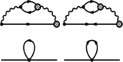
Figure 1: Top panel: The baryon Fock-exchange self-energies for normal (left graph) and anomalous (right graph) sectors. The solid lines correspond to the fermions, the wavy lines - to the pions; the blobs schematically indicate the RPA renormalized vertices, the dots - the bare pion-nucleon vertices. Bottom panel: The normal and anomalous Hartree diagrams. The dots stand for the contact Landau interactions; the straight lines are shown for clarity.

The top panel in Fig. 1 shows the Fock diagrams corresponding to Eqs. (41) and (42); the exchange diagrams, which are related to the direct ones by crossing symmetry are not shown, but are taken into account in the definition of the polarization function (II). The bottom panel in Fig. 1 shows the Hartree diagrams which contribute to the mean field and the BCS interaction via the short-range component of the interaction (the contribution of the pions to these diagrams vanishes). The analytical expressions for the retarded components of the self-energies can be read off from the diagrams

$$\Sigma^{R}(\omega) = \int_{-\infty}^{\infty}\frac{d\bar{\omega}}{2\pi}\frac{\Sigma^{>}(\bar{\omega})-\Sigma^{<}(\bar{\omega})}{\omega-\bar{\omega}+i\eta},$$ (44)

$$= \int_{-\infty}^{\infty}\frac{d\bar{\omega}}{2\pi}\int_{0}^{\infty}\frac{d\omega^{\prime}}{2\pi}\frac{D^{>}(\omega^{\prime})G^{>}(\bar{\omega}-\omega^{\prime})-D^{<}(\bar{\omega})G^{<}(\bar{\omega}-\omega^{\prime})}{\omega-\bar{\omega}+i\eta},$$

$$\Delta^{R}(\omega) = \int_{-\infty}^{\infty}\frac{d\bar{\omega}}{2\pi}\frac{\Delta^{>}(\bar{\omega})-\Delta^{<}(\bar{\omega})}{\omega-\bar{\omega}+i\eta}$$ (45)

$$= \int_{-\infty}^{\infty}\frac{d\bar{\omega}}{2\pi}\int_{0}^{\infty}\frac{d\omega^{\prime}}{2\pi}\frac{D^{>}(\omega^{\prime})F^{\dagger>}(\bar{\omega}-\omega^{\prime})-D^{<}(\bar{\omega})F^{\dagger<}(\bar{\omega}-\omega^{\prime})}{\omega-\bar{\omega}+i\eta},$$

where we used the dispersion relations for the retarded self-energies $\Sigma^{R}(\omega)$ and $\Delta^{R}(\omega)$ [in Eqs. (44) and (45) the momentum variables and the vertices have been suppressed]. Substituting the spectral representations of the Green’s functions in the above expression we arrive at

$$\Sigma^{R}(\omega,\bm{p}) = {\rm Tr}\int\!\!\frac{d^{3}q}{(2\pi)^{3}}\int_{-\infty}^{\infty}\!\!\frac{d\varepsilon}{2\pi}\Gamma_{0}(\bm{q})A_{G}(\varepsilon,\bm{p}-\bm{q})C(\omega,\varepsilon,\bm{q})\Gamma(\bm{q}),$$ (46)

$$\Delta^{R}(\omega,\bm{p}) = {\rm Tr}\int\!\!\frac{d^{3}q}{(2\pi)^{3}}\int_{-\infty}^{\infty}\!\!\frac{d\varepsilon}{2\pi}\Gamma_{0}(\bm{q})A_{F}(\varepsilon,\bm{p}-\bm{q})C(\omega,\varepsilon,\bm{q})\Gamma(\bm{q}),$$ (47)

where

$$C(\omega,\varepsilon,\bm{q})=\int_{0}^{\infty}\!\!\frac{d\omega^{\prime}}{2\pi}B(\omega^{\prime},\bm{q})\left[\frac{f(\varepsilon)+g(\omega^{\prime})}{\varepsilon-\omega^{\prime}-\omega-i\eta}+\frac{1-f(\varepsilon)+g(\omega^{\prime})}{\varepsilon+\omega^{\prime}-\omega-i\eta}\right].$$ (48)

The expressions (46)-(48) for the Fock self-energies are general to the extent that the approximations to the spectral function of pions and the pion-nucleon vertices have not been specified. In the numerical computations below we shall use the RPA renormalized spectral function of pions and the one-pion-exchange vertices which are dressed by the short-range correlations; clearly, our choice of the resummation scheme is not unique, but it is known to include the dominant set of graphs that renormalize the modes related to the long-range perturbations.

Next we proceed to integrate out the dependence of the self-energies on the on-shell energies by implementing the improved quasiclassical approximation (IQCA), which is described in the Appendix. Since at low temperatures the particle momenta lie close to their Fermi surface, the quasiclassical approximation (QCA), in its common form, expands the functions with respect to the small parameter $\delta p/p_{F}$, where $\delta p=|p-p_{F}|$ is the deviation of the particle momenta from their value on the Fermi surface, and keeps the zeroth order in $\delta p$ terms. Thus, the on-mass-shell physics is constrained to the Fermi surface because of the degeneracy of the system. Independently, the QCA assumes that the typical off-shell excitation energies are much smaller than the Fermi energy, so that the momentum integrals over the Green’s functions can be evaluated within infinite limits. The IQCA avoids the latter approximation since, as we shall see below, the off-shell excitation energies are of the same order of magnitude as the Fermi energy.

Upon implementing the IQCA, Eqs. (46) and (47) can be written as

$$\Sigma^{Q}(p_{F},\omega) = -\int_{0}^{\infty}d\omega^{\prime}K(\omega^{\prime})\Bigl{\{}g(\omega^{\prime})\left[G^{Q}(\omega+\omega^{\prime})+G^{Q}(\omega-\omega^{\prime})\right]$$ (49)

$$+\int_{-\infty}^{\infty}\frac{d\varepsilon}{\pi}{\rm Im~{}}[G^{Q}(\varepsilon)]J(\omega,\omega^{\prime},\varepsilon)\Bigr{\}},$$

$$\Delta^{Q}(p_{F},\omega) = \int_{0}^{\infty}d\omega^{\prime}K(\omega^{\prime})\Bigl{\{}g(\omega^{\prime})\left[F^{Q}(\omega+\omega^{\prime})+F^{Q}(\omega-\omega^{\prime})\right]$$ (50)

$$+\int_{-\infty}^{\infty}\frac{d\varepsilon}{\pi}{\rm Im~{}}[F^{Q}(\varepsilon)]J(\omega,\omega^{\prime},\varepsilon)\Bigr{\}},$$

where $\Sigma^{Q}(\omega,p_{F})$ and $\Delta^{Q}(\omega,p_{F})$ are the quasiclassical counterparts of the retarded self-energies,

$$J(\varepsilon,\omega,\omega^{\prime})=\frac{f(\varepsilon)}{\varepsilon-\omega-\omega^{\prime}-i\eta}+\frac{1-f(\varepsilon)}{\varepsilon-\omega+\omega^{\prime}-i\eta},$$ (51)

and we defined a momentum averaged (real) interaction kernel as

$$K(\omega)=\frac{m^{*}}{(2\pi)^{3}p_{F}}\int_{0}^{2p_{F}}dq~{}q\int_{0}^{2\pi}d\phi~{}B(\bm{q},\omega)~{}{\rm Tr}~{}\{\Gamma_{0}(\bm{q})\Gamma(\bm{q})\}.$$ (52)

Formally, Eqs. (49) and (50) are a coupled set of nonlinear integral equations for the complex pairing amplitude and the normal self-energy (i.e. are equivalent to four integral equations for four real quantities). This becomes explicit if we note that the Green’s functions on the right-hand side of Eqs. (49) and (50) can be expressed in terms of certain integrals

$$G^{Q}(\omega)=\omega Z^{Q}(\omega)I_{1}(\omega)+I_{2}(\omega),\quad F^{Q}(\omega)=-\Delta^{Q}I_{1}(\omega),$$ (53)

which are defined by Eqs. (Appendix) and (72) of the Appendix and are functions of the pairing field $\Delta^{Q}(p_{F},\omega)$ and the wave-function renormalization $Z^{Q}(p_{F},\omega)$. Let us briefly comment on the physical content of Eqs. (49) and (50). They describe the pairing and wave-function renormalization among degenerate fermions which live on their Fermi surface and interact via a force that depends on the momentum transfer. The effective pairing interaction $K(\omega)$ is an average over the momentum transfers that are accessible to particles constrained to their Fermi surface ($0\leq q\leq 2p_{F}$) with a weight given by the pion spectral function (i.e., the probability of finding a pion of momentum $\bm{q}$ at a fixed energy $\omega$). Although the function $K(\omega)$ is independent of momentum, it is not equivalent to a contact approximation to the (nonretarded) $S$-wave interaction in the potential models; the latter would correspond, in the present context, to the limit of zero momentum transfer. Let us recall again that the interaction kernel, via the momentum averaged spectral function of pions, incorporates the modification of the pionic spectrum by the nuclear medium - a feature that is missing in the potential models.

We turn now to the anomalous Hartree contribution, shown by the second diagram in the lower panel of Fig. 1 (the first diagram renormalizes the on-shell particle mass). Approximating the $S$-wave interaction in terms of the Landau parametrization, $F_{0}(\omega,\bm{q})+G_{0}(\omega,\bm{q})({\bm{\sigma}}_{1}\cdot{\bm{\sigma}}_{2})$, one finds for the mean-field BCS contribution to the pairing in the spin-zero state

$$\Delta^{R}_{BCS}(\omega,\bm{p}) = -i\int\frac{d^{4}p^{\prime}}{(2\pi)^{4}}[F_{0}(\omega^{\prime},\bm{p}^{\prime})-3G_{0}(\omega^{\prime},\bm{p}^{\prime})]$$ (54)

$$\times F^{\dagger<}(\omega+\omega^{\prime},\bm{p}+\bm{p}^{\prime}).$$

If the Landau parameters are further approximated by constants, the quasiclassical approximation to the Hartree self-energy becomes

$$\Delta_{BCS}^{Q}=(F_{0}-3G_{0})\nu(\mu)\int_{-\infty}^{\infty}\frac{d\omega}{\pi}f(\omega){\rm Im~{}}[F^{Q}(\omega)],$$ (55)

where $\nu(\mu)=p_{F}m^{*}/(2\pi^{2})$ is the density of states at the Fermi surface.

In the zero-temperature limit, Eqs. (49) and (50) take the simple form

$$Z^{Q}(\omega) = 1-\frac{1}{\omega}\int_{-\infty}^{\infty}\frac{d\varepsilon}{\pi}~{}{\rm Im}\left[G^{Q}(\varepsilon)\right]\,L(\omega,\varepsilon),$$ (56)

$$\Delta^{Q}(\omega) = \int_{-\infty}^{\infty}\frac{d\varepsilon}{\pi}~{}{\rm Im}\left[F^{Q}(\varepsilon)\right]\,L(\omega,\varepsilon),$$ (57)

where the effective (complex) retarded interaction is defined as

$$L(\omega,\varepsilon)=\int_{0}^{\infty}d\omega^{\prime}K(\omega^{\prime})\left[\frac{\theta(\varepsilon)}{\varepsilon-\omega+\omega^{\prime}-i\eta}+\frac{\theta(-\varepsilon)}{\varepsilon-\omega-\omega^{\prime}-i\eta}\right],$$ (58)

where $\theta(\varepsilon)$ is the Heaviside’s step function. Note that the thermal occupation probability of the pions vanishes in the zero-temperature limit and they contribute only to the effective interaction $L(\omega,\varepsilon)$. Note also that due to the time-reversal symmetry of the problem the energy integrations in Eqs. (56) and (57) can be restricted to the positive energy domain upon using the property $\Delta^{Q}(-\varepsilon)=\Delta^{Q}(\varepsilon)$, the time-reversal properties of the quasiclassical propagators (see the Appendix) and the symmetries of the effective interaction $L(\omega,\varepsilon)$. The form of Eq. (56) remains the same, but the effective interaction is replaced according to $L(\omega,\varepsilon)\to L_{-}(\omega,\varepsilon)$, while Eq. (57) becomes

$$\Delta^{Q}(\omega) = \int_{0}^{\infty}\frac{d\varepsilon}{\pi}~{}\left\{{\rm Im}\left[F_{\rm odd}^{Q}(\varepsilon)\right]\,L_{+}(\omega,\varepsilon)+~{}{\rm Im}\left[F_{\rm even}^{Q}(\varepsilon)\right]\,L_{-}(\omega,\varepsilon)\right\},$$ (59)

where the subscripts on the propagators refer to their odd and even in the energy variable parts and the new kernels are defined as

$$L_{\pm}(\omega,\varepsilon)=\int_{0}^{\infty}d\omega^{\prime}K(\omega^{\prime})\left[\frac{1}{\varepsilon+\omega+\omega^{\prime}+i\eta}\pm\frac{1}{\varepsilon-\omega+\omega^{\prime}-i\eta}\right].$$ (60)

The zero-temperature expression for the BCS contribution to the pairing gap becomes

$$\Delta_{BCS}^{Q}=(F_{0}-3G_{0})\nu(\mu)\int_{0}^{\infty}\frac{d\varepsilon}{\pi}\left\{{\rm Im~{}}[F_{\rm even}^{Q}(\varepsilon)]-{\rm Im~{}}[F_{\rm odd}^{Q}(\varepsilon)]\right\}.$$

The net pairing gaps in the quasiparticle spectrum is the sum of the Fock-exchange and Hartree terms $\Delta(\omega)\equiv\Delta^{Q}(\omega)+\Delta_{BCS}^{Q}$, defined by Eqs. (59) and (II).

III The algorithm and results

Equations (56) and (57) form a coupled set of four nonlinear integral equations for four real functions: these are the real and imaginary parts of the gap function $\Delta_{1}(\omega)$ and $\Delta_{2}(\omega)$, and the real and imaginary parts of the wave-function renormalization $Z_{1}(\omega)$ and $Z_{2}(\omega)$. Since the interaction kernel $L(\omega,\varepsilon)$ is constructed from the spectral function of pions, renormalized by the nuclear medium in the normal state, it serves as an input to Eqs. (56) and (57) and can be computed prior to their solution. Thus, as a first step, the $L(\omega,\varepsilon)$ function is generated on a two-dimensional energy grid. The starting point is the construction of the pion-spectral function from the real and imaginary parts of the RPA renormalized polarization function. The RPA polarization function is in turn constructed from the free-particle polarization function (or the Lindhard function) which has an analytical form both at zero and finite temperatures. From the pion spectral function and the RPA renormalized vertex $\Gamma(q)$ we then construct the momentum-averaged effective interaction $K(\omega)$ according to Eq. (52) in a typical energy range $0\leq\omega\leq 200$ MeV. The first part of the computation is accomplished by constructing the real and imaginary parts of the function $L(\omega,\varepsilon)$ on a two-dimensional energy grid. Typical computations were carried out on a $100\times 100$ point mesh. The range of energy integrations was extended up to 400 MeV to ensure that the integrands in Eqs. (56) and (57) have dropped to values below the accuracy of the integration. Note that the evaluation of Eq. (58) requires principle value integrations due to the simple poles in the integrand and, in addition, evaluation of integrals which are singular at the boundary.

In the second part of the computation the four integral equations represented by Eqs. (56) and (57) are solved self-consistently using as an input the values of the function $L(\omega,\varepsilon)$ stored on a two-dimensional energy grid. An iterative procedure is used. The iteration starts by assigning to the functions the values $\Delta_{1}(\omega)=$ const, $\Delta_{2}(\omega)=0$, $Z_{1}(\omega)=1$ and $Z_{2}(\omega)=0$, where the constant is set equal to the typical scale $\sim 1$ MeV. The newly computed functions are reinserted in the kernels on the right-hand side of the equations and the iterations are repeated until convergence is achieved. Note that the kernels of Eqs. (56) and (57) are singular; in the first of these equations the singularity is always at the lower boundary of the integration region, while in the second equation singularities occur both at the lower end point and within the integration regions (the latter is understood in the Cauchy sense). The positions of the singularities, of course, change from one iteration to another. An efficient use of the quadratures can be achieved by dividing the integration region into subintervals: a 24 point Clenshaw-Curtis integration was used on the intervals which contain singularities; in the remainder intervals the standard Gaussian rule was used. A few iterations were sufficient to achieve a convergence to accuracy $10^{-5}$ on all points of the energy mesh.

Below, we present the results obtained for zero-temperature low-density neutron matter relevant to the physics of neutron star crusts. The density is parametrized in terms of the Fermi momentum $\rho=p_{F}^{3}/(3\pi^{2})$ and we consider the range $0.4\leq p_{F}\leq 0.6$ fm ^-1 which is below the maximum of the on-shell pairing gap at about $p_{F}\simeq 1$ fm^-1. The gap decreases at larger densities due to the repulsive component of the pairing force and we need to include (at least) $\rho$-meson-exchange to reproduce this feature. We supplement our input parameters with a set of dimensionless (i.e., normalized by the density of states) Landau parameters. We keep them constant throughout the range of Fermi momenta considered. The effective Landau mass is set to $m^{*}/m=0.8$ and we assume $g^{\prime}=0.6$, although we discuss its variations towards the end of this section. To evaluate the BCS contribution (55) we choose the parameter values $f_{0}=-0.3$ and $g_{0}=0.3$ which are taken from Ref. WAMBACH1 . These values of Landau parameters satisfy the well-know stability criteria.

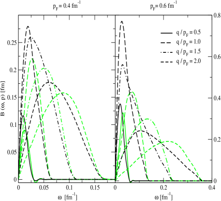
Figure 2: The frequency dependence of the free (light lines) and RPA renormalized (heavy lines) pion spectral function at several fixed values of the momentum transfer $q/p_{F}=0.5$, 1.0, 1.5 and 2.0. The density corresponds to $p_{F}=0.4$ fm^-1 in the left panel and to $p_{F}=0.6$ fm^-1 in the right panel.

Figure 2 displays the frequency dependence of the spectral function of pions at several fixed momentum transfers for densities corresponding to $p_{F}=0.4$ (left panel) and 0.6 fm^-1 (right panel). It can be seen that the contribution of processes with momentum transfers $q\leq p_{F}/2$ to the spectral function is unimportant compared to the contribution from large momentum transfers $q\geq p_{F}$. At fixed $q$ the spectral function has a Lorentzian shape as a function of energy transfer. For very large momentum transfers $q\leq 2p_{F}$, as the particle-hole excitations with higher energies become accessible, the spectral function is broadened and its maximum is shifted towards larger energies. Compared to the free case, the maximum of the spectral functions computed within the RPA is shifted to lower energies while the width remains nearly constant.

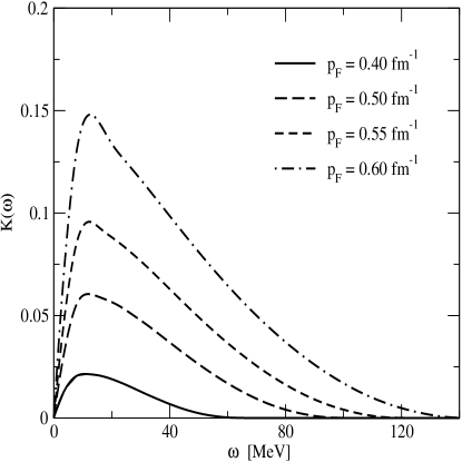
Figure 3: The frequency dependence of the averaged over the momentum transfer (dimensionless) kernel $K(\omega)$ derived from the RPA renormalized pion spectral function for $p_{F}=$ 0.4 (solid), 0.5 (long-dashed), 0.55 (dashed) and 0.6 (dashed-dotted lines).

Figure 3 displays the frequency dependence of the interaction kernel $K(\omega)$ for several Fermi momenta. The shape of the kernel $K(\omega)$ is Lorentzian at low and intermediate energies [characteristic also to spectral function $B(\bm{q},\omega)$ for fixed values of $|q|$] with an excess contribution in the high-energy tail. The contribution from small momentum transfers $q\ll p_{F}$ to the kernel $K(\omega)$ is negligible, since the spectral function for these processes is generally small (see Fig. 2) and, in addition, the integrand in Eq. (52) is weighted by the factor $q^{3}$, with each pion-nucleon vertex contributing a power of $q$. The latter factor cuts off the contribution from small momentum transfers. The main contribution to the peak of $K(\omega)$ function originates from the momentum transfers $|q|\sim p_{F}$; in this regime the maximum of the spectral function coincides with that of the $K(\omega)$ function. The excess contribution to the high-energy tail of the $K(\omega)$ function is due to the excitations with large momentum transfers and the magnifying effect of the pion-nucleon vertices (a factor $\propto q^{2}$). As the density is increased, the $K(\omega)$ function extends to higher energies, its maximum increase by roughly an order of magnitude over the Fermi momentum range $0.4\leq p_{F}\leq 0.6$ fm^-1 with a minor shift of its position to the higher energies. Note that the observed increase in the interaction strength will saturate at densities corresponding to $p_{F}\leq 1$ fm^-1 once the repulsive interaction via $\rho$ meson-exchange will become important.

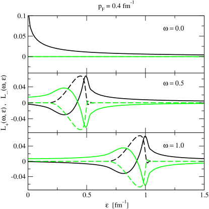
Figure 4: The $\varepsilon$-dependence of the effective interaction kernels $L_{+}(\omega,\varepsilon)$ (heavy lines) and $L_{-}(\omega,\varepsilon)$ (light lines) for fixed values of $\omega=0$, 0.5, and 1 fm^-1 for $p_{F}=0.4$ fm^-1. The solid and dashed lines refer to the real and imaginary parts.

The panels in Fig. 4 show the energy dependence of the real and imaginary parts of the interaction kernels $L_{\pm}(\omega,\varepsilon)$ [Eq. (60)] at several fixed values of the integration variable $\varepsilon$. Separating the real and imaginary parts in Eq. (60) it is easy to see that (i) the real parts acquire their maximum when $\varepsilon=\omega$ and (ii) the imaginary parts vanish for $\varepsilon\geq\omega$ features that are evident in Fig. 4. Thus, the main contribution to the kernel of the gap equation comes from the ‘diagonal’ part of the interaction kernel $L_{\pm}(\varepsilon,\varepsilon)$.

The frequency dependence of the real and imaginary parts of the gap function and the wave-function renormalization is shown in Fig. 5. The gap function has been replaced by a new function $\Delta^{\prime}(\omega)=Z^{-1}(\omega)\Delta(\omega)$ (the prime is dropped below), which is equivalent to a redefinition of the energy scale $\omega^{\prime}=\omega Z(\omega)$. The $\omega\to 0$ limit of these functions is consistent with what is known from the on-shell physics. The real part of the gap function $\Delta_{1}(\omega=0)$ is of the order of MeV and increases with density, as is the case for the pairing gaps deduced using potential models. The real part of the wave-function renormalization $Z_{1}(\omega=0)$ is larger than unity, i.e., there is an enhancement of the density of states at the Fermi surface. The imaginary parts of these functions vanish in the limit $\omega\to 0$ (as they should). Off the mass-shell the real and imaginary parts of the gap function develop a complicated structure: in the low-energy domain, below the maximum of the function $K(\omega)$ at about 10 MeV, the real part of the gap function dominates the imaginary part: $|\Delta_{1}(\omega)|>|\Delta_{2}(\omega)|$. Beyond the maximum the opposite is true up to the energies $\omega\simeq 100$ MeV.

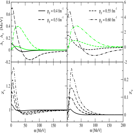
Figure 5: Top panel: The frequency dependence of the real (heavy lines) and imaginary (light lines) parts of the gap function $\Delta_{1}(\omega)$ and $\Delta_{2}(\omega)$ for $p_{F}=0.4$ (solid) 0.5 (long-dashed) 0.55 (dashed) and 0.6 (dashed-dotted lines) fm^-1. The on-shell values of the pairing gap are 0.1, 0.7, 1.4, and 3.7 MeV for $p_{F}=0.4$, 0.5, 0.55 and 0.6 fm^-1. Bottom panel: The frequency dependence of the real (left panel) and imaginary (right panel) parts of the wave-function renormalization $Z_{1}(\omega)$ and $Z_{2}(\omega)$. The labeling is the same as in the top panel.

A nonvanishing imaginary part $\Delta_{2}(\omega)$ implies a finite decay time for the pairing correlations due to the coupling of the neutron quasiparticles to the pionic modes. The imaginary part of the wave-function renormalization $Z_{2}(\omega)$ implies, likewise, finite lifetime for the normal quasiparticle excitation. It is worthwhile to note that the latter effect is not independent of the pairing correlations, since it emerges from a self-consistent solution of the coupled dynamics of the normal and anomalous sectors. The enhancement of the gap and the wave-function renormalization with increasing density can be traced back to the enhancement of the attractive interaction kernel $K(\omega)$. Including the repulsive components of the interaction by treating heavier (notably $\rho$ meson) exchanges would lead to a saturation of the attractive interactions at about $p_{F}\simeq 1$ fm^-1 and a depression of the gap at larger densities.

Many-body calculations of the Landau parameters lead to values $g^{\prime}\simeq 0.6-0.8$ Dickhoff:qr ; Dickhoff:qr2 ; Dickhoff:qr3 . The experimental evidence from the studies of spin-isospin modes in finite nuclei suggests that $g^{\prime}\simeq 0.6$.

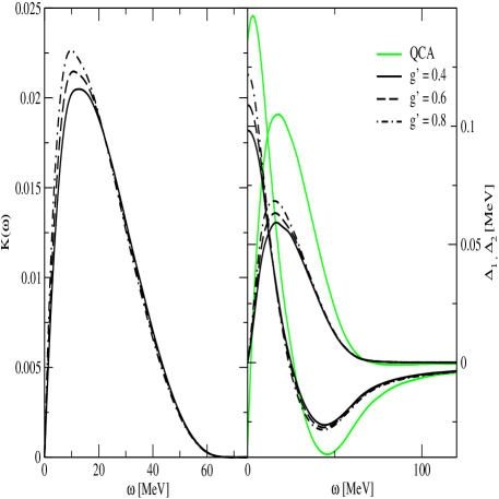
Figure 6: The frequency dependence of the effective interaction kernel $K(\omega)$ (left graph) and the real $\Delta_{1}(\omega)$ and imaginary $\Delta_{2}(\omega)$ parts of the pairing gap (right graph) for three values of the Landau parameter $g^{\prime}=0.4$, 0.6 and 0.8 and $p_{F}=0.4$ fm^-1. The light lines correspond to the QCA approximation with $g^{\prime}=0.6$ for $p_{F}=0.4$ fm^-1.

Figure 6 displays the changes in the interaction kernel $K(\omega)$ and the pairing gap function $\Delta(\omega)$ as the Landau parameter $g^{\prime}$ is varied in the range 0.4-0.8. The larger $g^{\prime}$ the stronger is the attractive interaction kernel and, hence, the larger is the pairing gap. The overall range of variations of these quantities is, however, small and the observables are insensitive to the variations of $g^{\prime}$. As discussed in the Appendix, the ordinary QCA requires that the characteristic off-shell energies of the excitation be smaller than the Fermi energy $\omega/\mu\ll 1$ - a condition which is not well satisfied for excitation energies in the present model. One finds typically $\omega/\mu\sim 1$. The IQCA relaxes the $\omega/\mu\ll 1$ assumption of the QCA, but treats the pairing gaps and the wave-function renormalizations independent of the momentum variable. Figure 6 (right panel) compares the results obtained within the QCA and the IQCA. Although the qualitative picture is the same in both approximations, the IQCA leads to smaller gap functions (and wave-function renormalizations) because the integrations over the on-mass-shell energy are limited to a finite shell, while the QCA assumes infinite integration limits. Calculations which include full momentum dependence of the gap function and wave-function renormalization will be needed to gauge the remaining error due to the IQCA.

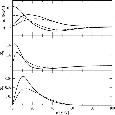
Figure 7: The frequency dependence of the real $\Delta_{1}(\omega)$ and imaginary $\Delta_{2}(\omega)$ parts of the pairing gap (top panel) and the real $Z_{1}(\omega)$ and imaginary $Z_{2}(\omega)$ parts of wave-function renormalization (bottom panels) for $p_{F}=0.4$ fm^-1. The solid and dashed curves correspond to the results obtained with the RPA renormalized and free pion spectral function.

Finally, Fig. 7 compares the results obtained with the free and the RPA renormalized pion spectral function. The shapes of the gap and renormalizations functions are qualitatively similar in both cases; however, the RPA renormalization enhances the values of the gap at small frequencies and, therefore, their on-shell values. More generally, according to Fig. 7, the RPA renormalization enhances (suppresses) the gap and renormalization functions in the low-frequency (high-frequency) limit. These features are consistent with the frequency dependence of the free and renormalized spectral functions displayed in Fig. 2.

IV Concluding remarks

In this work we proposed a model of pairing in nuclear systems based on the meson-exchange picture of nuclear interactions that includes retardation effects. The model is illustrated on a simplest possible example - neutrons interacting via exchange of neutral pions; the short-range correlations are included in the spirit of Landau-Migdal theory of Fermi liquids. Unlike the treatments based on the potential models, the modifications of the meson properties in the medium are taken into account by relating the pairing gap function and the wave-function renormalization to the spectral functions of mesons. We computed these medium modifications for the pionic modes within the non-perturbative particle-hole (RPA) resummation scheme, which softens their spectrum, but has no qualitative effect on the retardation. The model builds in the retardation effect via the coupled Fock-exchange self-energies for normal and anomalous sectors. The Hartree self-energies receive contributions only from the short-range part of the interaction, as pions do not contribute. Although we obtain the exact self-energies for our system, these are solved numerically with the improved quasiclassical approximation (IQCA). Since it is difficult to estimate a priori the error introduced through the IQCA (which fixes the momentum transfer at the Fermi momentum) our numerical results should be taken with caution.

The numerical calculations above show that the real and imaginary parts of the gap function are of the same order of magnitude over a wide energy range. At low energies, the real part of the gap function dominates the imaginary part, i.e., the Fourier transform of the anomalous pair-correlation function in the time-domain shows a damped oscillatory behavior; the picture is opposite in the high-energy regime, typically above tens of MeV, where the oscillations are damped out within a ‘cycle’. Physically, the complex pairing gap implies a finite lifetime of the Cooper pairs due to the emission/absorption of pions. The real part of the wave-function renormalization (derived self-consistently with the gap equation) is larger than unity, i.e., implies an enhancement of the density of states; the finite imaginary part describes the damping of the normal quasiparticle excitations due to the coupling to the pion modes. The frequency dependence of the pairing gap and the wave-function renormalization will have implications on the responses of nuclear systems to those electromagnetic and weak probes which are sensitive to the energy range where these functions vary substantially.

Extrapolating from the analysis of this paper, it is clear that the meson-exchange picture of pairing with retardation can be extended to treat problems which have been difficult to handle within the potential models. Such an extension could incorporate the dynamics of nucleon resonances, for example, to clarify the role of delta’s in the effective retarded interaction or to deduce their pairing properties. Another interesting direction is the application of the model to the strange sector to study the pairing properties of the strange baryons that are stable in the interiors of compact stars (typically $\Sigma$ and $\Lambda$ hyperons, see Ref. GLENDENNING ; WEBER ), the role of the kaon dynamics on the pairing properties of the strange baryons, etc. The model appears also suitable for treating the fermionic pair condensation of the baryons on the same footing with the Bose condensation of pions or kaons.

Appendix

The purpose of this appendix is to discuss in detail the approximations to the full normal and anomalous Green’s functions that allow us to remove the explicit momentum dependence of the wave-function renormalization and the gap function. We start by examining the momentum dependence of Eqs. (46)-(48) in the low-temperature limit. Since the formal structure of the normal and anomalous self-energies is the same, we shall apply our arguments only to the normal self-energy, Eq. (46). Below, we assume isotropic medium with a spherical Fermi surface.

Using the spectral representations of the Green’s functions (28) and (29), Eq. (46) can be transformed to the following form

$$\Sigma^{R}(\omega,\bm{p})=\int\frac{d^{3}q}{(2\pi)^{3}}{\rm Tr}\{\Gamma_{0}(\bm{q})\Gamma(\bm{q})\}\int_{0}^{\infty}\frac{d\omega^{\prime}}{2\pi}B(\omega^{\prime},\bm{q})\Biggl{[}g(\omega^{\prime})G^{R}(\bm{p}-\bm{q},\omega+\omega^{\prime})$$

$$-g(\omega^{\prime})G^{R}(\bm{p}-\bm{q},\omega-\omega^{\prime})+\int_{-\infty}^{\infty}\frac{d\varepsilon}{\pi}J(\varepsilon,\omega,\omega^{\prime}){\rm Im}G^{R}(\bm{p}-\bm{q},\epsilon)\Biggl{]},$$ (62)

where the function $J(\varepsilon,\omega,\omega^{\prime})$ is defined by Eq. (51). Directing the axis of a spherical system of coordinates along the vector $\bm{p}$, the integration measure becomes $d^{3}q=q^{2}dq~{}dx~{}d\phi$, where $x$ is the cosine of the angle between the vectors $\bm{p}$ and $\bm{q}$. Upon defining $\bm{k}=\bm{p}-\bm{q}$ and replacing the integration over $x$ by an integration over $\xi_{k}$, Eq. (Appendix) becomes

$$\Sigma^{R}(\omega,p_{F})=\frac{m^{*}}{(2\pi)^{2}p_{F}}\int_{0}^{\infty}\!\!qdq{\rm Tr}\{\Gamma_{0}(\bm{q})\Gamma(\bm{q})\}\int_{0}^{\infty}\frac{d\omega^{\prime}}{2\pi}B(\omega^{\prime},\bm{q})H(\omega,\omega^{\prime}),$$ (63)

with

$$H(\omega,\omega^{\prime}) = g(\omega^{\prime})\int_{\xi_{-}(q)}^{\xi_{+}(q)}\!\!d\xi_{k}~{}[G^{R}(\bm{k},\omega+\omega^{\prime})+G^{R}(\bm{k},\omega-\omega^{\prime})]$$ (64)

$$+ \int_{-\infty}^{\infty}\frac{d\varepsilon}{\pi}J(\varepsilon,\omega,\omega^{\prime})\int_{\xi_{-}(q)}^{\xi_{+}(q)}\!\!d\xi_{k}~{}{\rm Im}G^{R}(\bm{k},\epsilon),$$

where $\xi_{k}=k^{2}/2m^{*}-\mu$, the integration limits are $\xi_{\pm}=(p_{F}\pm q)^{2}/2m^{*}-\mu$, $m^{*}$ is the effective mass, $\mu$ is the chemical potential. Without loss of generality, the momentum argument of the self-energy $\Sigma^{R}(\omega,p)$ is taken as the Fermi momentum, i.e., the expressions (63) and (64) are still exact.

Quasiclassical Green’s functions. Now we turn to the $\xi_{k}$-integrations in Eq. (64). Formally, the quasiclassical approximation (QCA) amounts to (i) taking infinite limits $\xi_{\pm}\to\pm\infty$ and (ii) approximating the function $\Delta(\xi_{k},\omega)$ and $Z(\xi_{k},\omega)$ in the propagators by their values on the Fermi surface $\Delta(\xi(p_{F}),\omega)$ and $Z(\xi(p_{F}),\omega)$. The integrals over the normal and anomalous Green’s functions are then computed by a contour integration

$$\int_{-\infty}^{\infty}\!\!d\xi_{k}~{}\frac{\omega Z(\omega)+\xi_{k}}{\omega^{2}Z(\omega)^{2}-\xi_{k}^{2}-\Delta^{R}(\omega)^{2}+i~{}{\rm sgn}(\omega)\eta}$$ (66)

$$\hskip 56.9055pt=-i\pi\frac{\omega Z(\omega){\rm sgn}(\omega)}{\sqrt{\omega^{2}Z^{2}(\omega)-\Delta(\omega)^{2}}}~{}\theta[\omega^{2}Z^{2}(\omega)-\Delta(\omega)^{2}],$$

$$\int_{-\infty}^{\infty}\!\!d\xi_{k}~{}\frac{-\Delta^{R}(\omega)}{\omega^{2}Z(\omega)^{2}-\xi_{k}^{2}-\Delta^{R}(\omega)^{2}+i~{}{\rm sgn}(\omega)\eta}$$

$$\hskip 56.9055pt=i\pi\frac{\Delta(\omega){\rm sgn}(\omega)}{\sqrt{\omega^{2}Z^{2}(\omega)-\Delta(\omega)^{2}}}~{}\theta[\omega^{2}Z^{2}(\omega)-\Delta(\omega)^{2}].$$

The second approximation [$\xi(k)\to\xi(k_{F})$], assumes that the gap function and the wave-function renormalization are smooth functions of momentum, therefore, at low temperatures, they can be approximated by their values at the Fermi surface. For the range of possible momentum transfers $0\leq q\leq 2p_{F}$ for particles on their Fermi surface, the functions need to be constant in the interval $k\in[0~{};~{}3p_{F}]$. Such an assumption is not inconsistent with the results of the potential models, but an error estimate will depend on the shape of the chosen interaction in the momentum space. Note that in our case, the momentum dependence of the functions is controlled by the shape of the spectral function which contributes mainly for $q\geq p_{F}$.

The first approximation (infinite integration limits) uses the fact that the large momentum transfers are important in the integration in Eq. (63), so that the limits $|\xi_{\pm}|\sim\mu$ are large compared to values of the poles of the Green’s functions in Eqs. (66) and (66), i.e., the condition $\xi_{\rm pole}\ll|\xi_{\pm}|$ is satisfied. The main contribution to the $q$ integration comes from large momentum transfers $p_{F}\leq q\leq 2p_{F}$ (see Sec. III), so that $\xi_{\pm}=(p_{F}\pm q)^{2}/2m^{*}-\mu\sim\pm\mu$ [note that max $(\xi_{+})=8\mu$ and min $(\xi_{-})=-\mu$]. In addition, the pion-nucleon vertices contribute a factor of $q^{2}$ to the integrand in Eq. (63), which cuts off the contributions from small momentum transfers. The poles of the Green’s functions in Eqs. (66) and (66) are defined by the condition $|\xi_{\rm pole}|=\sqrt{\omega^{2}Z(\omega)^{2}-\Delta(\omega)^{2}}\leq\omega$. The QCA is then applicable whenever the condition $\xi_{\rm pole}/\mu\ll 1$ is satisfied. In our problem, the typical energy scale for the off-shell excitations is of the order of 20 MeV which is of the same order of magnitude as the Fermi energies; the parameter $\xi_{\rm pole}/\mu$ could be of the order of unity, in which case the conventional QCA will break down.

Improved quasiclassical Green’s functions. Here we shall improve on the second approximation of the QCA by keeping the integration limits finite. To decouple the on-shell energy integrations over the Green’s functions from the remainder of the kernel, we approximate the $q$-dependent integration limits $\xi_{\pm}(q)$ by constants $\xi_{\pm}(p_{F})$. Setting the momentum transfer to $q=p_{F}$ is motivated by the shape of the pion-spectral function which, as noted above, contributes essentially in the range $p_{F}\leq q\leq 2p_{F}$.

The integrations in Eq. (64) and the analog equation for the anomalous self-energy require then two types of integrals ($\xi\equiv\xi_{k}$ hereafter)

$$I_{1} = \int_{\xi_{-}}^{\xi_{+}}\!\!\frac{d\xi}{\omega^{2}Z(\omega)^{2}-\xi^{2}-\Delta^{R}(\omega)^{2}+i~{}{\rm sgn}(\omega)\eta},$$ (67)

$$I_{2} = \int_{\xi_{-}}^{\xi_{+}}\!\!\frac{\xi~{}d\xi}{\omega^{2}Z(\omega)^{2}-\xi^{2}-\Delta^{R}(\omega)^{2}+i~{}{\rm sgn}(\omega)\eta}.$$ (68)

Upon defining a shorthand $D=\omega^{2}Z(\omega)^{2}-\Delta^{R}(\omega)^{2}$, the first integral can be rewritten as

$$I_{1} = \int_{\xi_{-}}^{\xi_{+}}\!\!d\xi_{k}\left[\frac{\theta(D)}{D-\xi^{2}+i~{}{\rm sgn}(\omega)\eta}+\frac{\theta(-D)}{D-\xi^{2}+i~{}{\rm sgn}(\omega)\eta}\right].$$ (69)

The first term contains a pole and we apply the Dirac identity $1/x=P/x-i\pi\delta(x)$ to separate the real and imaginary parts ($P$ stands for the principal value). The second term is regular and we take the limit $\eta\to 0$ to obtain

$$I_{1} = \int_{\xi_{-}}^{\xi_{+}}\!\!d\xi\Biggl{\{}\theta(D)\frac{P}{D-\xi^{2}}-\frac{\theta(-D)}{-D+\xi^{2}}-i\,\pi\,{\rm sgn}(\omega)\frac{\theta(D)}{2|\xi|}\left[\delta(\xi-\sqrt{D})+\delta(\xi+\sqrt{D})\right]\Biggr{\}}.$$

These integrals are standard (e.g. 3.3.21 and 3.3.23 of Ref. ABRAM ) and the final result is

$$I_{1} = \frac{\theta(D)}{2\sqrt{D}}~{}{\rm ln}\Bigg{|}\frac{(\sqrt{D}+\xi_{+})}{(\sqrt{D}-\xi_{+})}\frac{(\sqrt{D}+\xi_{-})}{(\sqrt{D}-\xi_{-})}\Bigg{|}+\frac{\theta(-D)}{\sqrt{D}}{\rm arctanh}\left[\frac{\xi_{+}+\xi_{-}}{\sqrt{D}(1+\xi_{+}\xi_{-})}\right]$$

$$- i\,\pi\,{\rm sgn}(\omega)\frac{\theta(D)}{2\sqrt{D}}\left\{\theta[(\xi_{+}-\sqrt{D})(\sqrt{D}-\xi_{-})]+\theta[(\xi_{+}+\sqrt{D})(-\sqrt{D}-\xi_{-})]\right\}.$$

The step functions in the last term insure that the poles of the propagators are counted only if they lie within the integration limits; to obtain the final expression we have used the relation arctan($ix)=i~{}$arctanh$(x)$. In the limit $\xi_{\pm}\to\pm\infty$ we recover the right-hand sides of Eqs. (66) and (66). The integral $I_{2}$ is computed as above and, upon using 3.3.22 of Ref. ABRAM , we obtain

$$I_{2}=\frac{1}{2}~{}{\rm ln}\Bigg{|}\frac{D-\xi_{-}^{2}}{D-\xi_{+}^{2}}\Bigg{|}\left[\theta(D)-\theta(-D)\right].$$ (72)

Note that this integral vanishes when the limits are infinite ($\xi_{\pm}\to\pm\infty$) or, more generally, when the integration is within finite limits which are symmetrical ($|\xi_{-}|=|\xi_{+}|)$. Under the time reversal the integrals $I_{1}$ and $I_{2}$ transform according to

$${\rm Re}~{}I_{1,2}(-\omega)={\rm Re}~{}I_{1,2}(\omega),\quad{\rm Im}~{}I_{1}(-\omega)=-{\rm Im}~{}I_{1}(\omega).$$ (73)

These transformation properties were used to derive Eqs. (59)-(II).

References

- (1) P. Ring and P. Schuck,The Nuclear Many Body Problem (Springer-Verlag, New York, 1980), Chaps. 4 and 7.
- (2) A. B. Migdal, Theory of Finite Fermi Systems and Applications to Atomic Nuclei (Interscience, London, 1967).
- (3) S. O. Bäckman, G. E. Brown, and J. A. Niskanen, Phys. Rep. 124, 1 (1985), and references therein.
- (4) W. H. Dickhoff, A. Faessler, H. Müther, and S. S. Wu, Nucl. Phys. A405, 534 (1983).
- (5) W. H. Dickhoff, A. Faessler, J. Meyer ter Vehn, and H. Müther, Phys. Rev. C 23, 1154 (1981).
- (6) W. H. Dickhoff and H. Müther, Nucl. Phys. A473, 394 (1987).
- (7) S. V. Babu and G. E. Brown, Ann. Phys. (N.Y.) 77, 1 (1973).
- (8) J. Wambach, T. L. Ainsworth, and D. Pines, Nucl. Phys. A555, 128 (1993).
- (9) T. L. Ainsworth, J. Wambach, and D. Pines, Phys. Lett. B 222, 173 (1989).
- (10) H.-J. Schulze, J. Cugnon, A. Lejeune, M. Baldo, and U. Lombardo, Phys. Lett., B 375, 1 (1996).
- (11) J. Clark, C.-G. Källman, C.-H. Yang, and D. Chakkalakal, Phys. Lett., B 61 331 (1976).
- (12) J. M. C. Chen, J. W. Clark, E. Krotschek, and R. A. Smith, Nucl. Phys. A451, 509 (1986).
- (13) J. M. C. Chen, J. W. Clark, R. D. Davé, and V. V. Khodel, Nucl. Phys. A555, 59 (1993).
- (14) M. Baldo and A. Grasso, Phys. Lett. B 485 115, (2000).
- (15) U. Lombardo, P. Schuck, and W. Zuo, Phys. Rev. C 64, 021301 (2001).
- (16) C. Shen, U. Lombardo, P. Schuck, W. Zuo, and N. Sandulescu, Phys. Rev. C 67 061302 (2003).
- (17) T. Alm, G. Röpke, A. Schnell, N. H. Kwong, and H. S. Köhler, Phys. Rev. C 53, 2181 (1996).
- (18) P. Bożek, Phys. Rev. C 62, 054316 (2000); 65, 034327 (2002).
- (19) A. Schwenk, B. Friman, and G. E. Brown, Nucl. Phys. A713, 191 (2003).
- (20) J. Kuckei, F. Montani, H. Müther, and A. Sedrakian, Nucl. Phys. A723, 32 (2003).
- (21) A. Sedrakian, T. T. S. Kuo, H. Müther, and P. Schuck, Phys. Lett. 576 68 (2003).
- (22) G. M. Eliashberg, Zh. Eksp. Teor. Fiz. 38, 966 (1960) [Sov. Phys. JETP 11, 696 (1960)].
- (23) J. R. Schrieffer, Theory of Superconductivity (Benjamin, New York, 1964), Chap. 7.
- (24) D. J. Scalapino, in Superconductivity, edited by R. D. Parks (Marcel Dekker, New York, 1969), Chap. 10.
- (25) G. D. Mahan, Many-Particle Physics (Plenum, New York, 1990), Chap. 9.
- (26) A. Sedrakian, in Proceedings International Workshop Hirshegg ’98, Nuclear Astrophysics, edited by M. Buballa, W. Nörenberg, J. Wambach, and A. Wirzba (GSI, Darmstadt 1998), p. 54, [astro-ph/9801239].
- (27) J. Terasaki, F. Barranco, R. A. Broglia, E. Vigezzi, and P.-F. Bortignon, Nucl. Phys. A697, 127 (2002).
- (28) A. V. Avdeenkov and S. P. Kamerdzhiev, JETP Lett. 69, 715 (1999) [Pis’ma Zh. Eksp. Teor. Fiz. 69, 669 (1999]; Yad. Fiz. 62, 610 (1999) [Phys. Atom. Nucl. 62, 563 (1999)]; Phys Lett. B 459, 423 (1999).
- (29) H. Kucharek and P. Ring, Z. Phys. A 339, 23 (1991).
- (30) F. B. Guimaraes, B. V. Carlson, and T. Frederico, Phys. Rev. C 54, 2385 (1996).
- (31) F. Matera, G. Fabbri, and A. Dellafiore, Phys. Rev. C 56, 228 (1997).
- (32) A. B. Migdal, Rev. Mod. Phys. 50, 10 (1978).
- (33) G. Baym, H. A. Bethe, and C. J. Pethick, Nucl. Phys. A175, 225 (1971).
- (34) J. W. Negele and D. Vautherin, Nucl. Phys. A207, 298 (1973).
- (35) For a review of the recent work see P. Haensel, in Physics of Neutron Star Interiors, edited D. Blaschke, N. K. Glendenning, and A. Sedrakian, (Springer-Verlag, New York, 2001), p. 127.
- (36) J. W. Serene and D. Reiner, Phys. Rep. 101, 221 (1983).
- (37) T. Ericson and W. Weise, Pions and Nuclei (Claredon Press, Oxford, 1988).
- (38) N. K. Glendenning, Compact Stars, 1st ed. (Springer-Verlag, New York, 1996)’ 2nd ed.(Springer-Verlag, New York, 2000).
- (39) F. Weber, Pulsars as Astrophysical Laboratories for Nuclear and Particle Physics (IOP, Bristol 1999).
- (40) M. Abramowitz and I. Stegun, Handbook of Mathematical Functions, (Dover, New York, 1972).