Electromagnetic interaction in chiral quantum hadrodynamics and decay of vector and axial-vector mesons

Abstract

The chiral invariant QHD-III model of Serot and Walecka is applied in the calculation of some meson properties. The electromagnetic interaction is included by extending the symmetry of the model to the local $U(1)\times SU(2)_{R}\times SU(2)_{L}$ group. The minimal and nonminimal contributions to the electromagnetic Lagrangian are obtained in a new representation of QHD-III. Strong decays of the axial-vector meson, $a_{1}\rightarrow\pi\rho,\,\ a_{1}\rightarrow\pi\sigma$, and the electromagnetic decays $\rho\rightarrow\pi\pi\gamma,\,\ a_{1}\rightarrow\pi\gamma$ and $\rho\rightarrow\pi\gamma$ are calculated. The low-energy parameters for the $\pi-\pi$ scattering are calculated in the tree-level approximation. The effect of the auxiliary Higgs bosons, introduced in QHD-III in order to generate masses of the vector and axial-vector mesons via the Higgs mechanism, is studied as well. This is done on the tree level for $\pi-\pi$ scattering and on the level of one-loop diagrams for the $a_{1}\rightarrow\pi\gamma$ decay. It is demonstrated that the model successfully describes some features of meson phenomenology in the non-strange sector.

I Introduction

Relativistic models built with hadronic degrees of freedom have been very successful in describing different properties of nuclei and hadrons at low and intermediate energies (for comprehensive reviews see refs. Ser86 ; Mei88 ; Ser97 ). In some of these models, the hadronic Lagrangian has symmetries which are inspired by the underlying QCD theory. This allows one to have fewer parameters, thereby reducing ambiguities in the hadronic models. One of the first models which incorporated the $SU(2)_{R}\times SU(2)_{L}$ symmetry was the gauged linear $\sigma$ model (GLSM) developed in ref. Lee68 . This model was an extension of the linear $\sigma$ model and included, in addition to the pion and scalar meson, the vector $\rho$ and axial-vector $a_{1}$ mesons as gauge bosons of the local $SU(2)_{R}\times SU(2)_{L}$ symmetry. The local symmetry was explicitly broken by the vector-meson mass terms, and spontaneous symmetry breaking (SSB) by the scalar field led to the mass splitting between the $\rho$ and $a_{1}.$ This model was elaborated in Gas69 , where the current-field identities were established. Later the model was applied Ko94 in a description of the meson properties. Because of some difficulties additional terms are often included. These terms break further the local symmetry and introduce additional parameters, which allow for a better description of the meson observables Gas69 ; Ko94 ; Urb01 .

The QHD-II model, which respects the local $SU(2)_{V}$ isospin symmetry, was developed in refs. Ser79 ; Ser86 . It was extended in ref. Ser92 by adding the chiral $SU(2)_{A}$ symmetry. This model, called QHD-III, is a chiral invariant theory based on the local symmetry $SU(2)_{R}\times SU(2)_{L}$. The $\rho$ and $a_{1}$ mesons are included as the gauge bosons which are initially massless. The masses are generated through SSB and the Higgs mechanism. The Lagrangian of QHD-III includes the Lagrangian of GLSM and the Lagrangian of the Higgs fields. The need for the latter sector of the model was clearly explained in ref. Pre99 : the Higgs mechanism in GLSM with local symmetry leads to the disappearance of the pion which plays the role of a would-be Goldstone boson giving its degree of freedom to the massive $a_{1}$ meson. Therefore the Higgs sector serves to generate the masses of the $a_{1}$ and $\rho$ mesons and to preserve the pion as a physical degree of freedom. Due to the local gauge symmetry the model is renormalizable and does not require the introduction of cut-off parameters. It is also parity conserving by construction.

A subtle aspect of QHD-III (but also of GLSM and other hadronic models including the axial-vector meson) is the presence of a bilinear term mixing the $a_{1}$ and pion fields. This considerably complicates the interpretation of the physical particles in the theory as well as calculations with this Lagrangian. One way to get rid of the mixing was considered in Lee68 and later used in other papers Gas69 ; Mei88 ; Ser92 ; Ko94 . It consists of a re-definition of the $a_{1}$ field and subsequent wave-function renormalization of the pion field. The final Lagrangian takes a complicated form with strongly momentum-dependent vertices. This has undesirable implications in low-energy meson phenomenology. As examples, we mention the vanishing of the $a_{1}\pi\rho$ and $\sigma\pi\pi$ vertices at some values of the invariant masses of the $a_{1}$ and $\sigma$, and the difficulties with the $\rho\pi\pi$ vertex Urb01 . The authors of Urb01 , instead of re-defining the fields, preferred to sum the self-energy generated by the  $a_{1}-\pi$ mixing to all orders.

An alternative method in the framework of QHD-III was recently suggested in Pre99 . This method exploits the freedom in choosing the gauge due to the local gauge invariance. Originally Ser92 the so-called unitary gauge was chosen from the beginning, and the two massless isovector Goldstone bosons (we will call them $\mathbf{H}$ and $\mathbf{Z}$) were ”gauged away”. This choice leads to the above-mentioned complication with the mixing. Note that the pseudoscalar boson $\mathbf{Z}$ has the same quantum numbers $I(J^{P})=1(0^{-})$ as the pion $\pi$ originating from GLSM sector. Therefore the physical pion field can be chosen as a linear combination of $\mathbf{Z}$ and $\pi$, while the orthogonal combination is decoupled in the unitary gauge Pre99 . The Lagrangian then takes a simpler form, without complicated momentum-dependent vertices.

In the present paper we apply this new representation of QHD-III in the calculation of some meson properties. First, we include the electromagnetic (EM) interaction in this model. This is done via an extension of the symmetry of QHD-III to the local $U(1)\times SU(2)_{R}\times SU(2)_{L}$ group. We use an arbitrary gauge where all eight Higgs fields are initially present. The EM interaction in both sectors of the model is obtained. After an appropriate diagonalization of the $\mathbf{Z}$ and $\pi$ fields and fixing the gauge along the lines of ref. Pre99 , we obtain the EM interaction in terms of the physical pion field. The final Lagrangian includes the minimal EM interaction, as well as the (nonminimal) EM interaction with the intrinsic magnetic moment of the $\rho$ and $a_{1}$ mesons.

We then study the strong and EM decays of the vector and axial-vector mesons. Some of the decays can be calculated on the “tree-graph” level, while others require a calculation beyond the tree level. In particular, we calculate the width of the following decays: $a_{1}\rightarrow\pi\rho\,,$ $a_{1}\rightarrow\pi\sigma$ and $\rho^{0}\rightarrow\pi^{+}\pi^{-}\gamma.$ We also address the issue of the width of the scalar $\sigma$ meson, in view of the interest Ko94 in this subject. The matrix elements for the above decays are given directly by the corresponding vertices in the Lagrangian. In order to calculate the decays $\ a_{1}^{+}\rightarrow\pi^{+}\gamma$ and $\ \rho^{+}\rightarrow\pi^{+}\gamma$ we need to include loop diagrams. In particular, the $a_{1}^{+}\rightarrow\pi^{+}\gamma$ process is described by a large number of one-loop diagrams, which can be grouped according to the intermediate state in the diagram. The diagrams where only vector or axial vector mesons in the loop are present are not yet included in this exploratory study.

All matrix elements of the EM processes turn out to be finite, due to a cancellation of divergencies between different amplitudes. The fulfillment of EM gauge invariance serves as a check of the calculation. The decay widths of these processes are listed in the PDG reviews, and we compare the model predictions with experimental values.

To determine the parameters of the model we fix the strong-coupling constant $g_{\rho}$ from the $\rho\rightarrow\pi\pi$ decay. All other parameters are strongly correlated, once the masses of the particles are taken equal to their experimental values. Only the mass $m_{\sigma}$ of the $\sigma$ meson and the mass $m_{H}$ of the Higgs particles remain unconstrained. The mass $m_{H}$ is taken to infinity in the calculation. As an additional test of the model we calculate the low-energy parameters for $\pi-\pi$ scattering. Because of some unusual features of the model, such as the presence of Higgs mesons and a suppression of the $\pi\pi\sigma$ interaction, it is not a priori clear whether the model can reasonably describe the experiment. The scattering lengths and effective ranges for the $S-$ and $P-$waves are calculated on the tree level and compared with the data and other approaches.

The paper is organized as follows. In Sect. II the Lagrangians of the EM and strong interactions are obtained. We start with the Higgs sector in Sect. II.1. The GLSM is briefly discussed in Sect. II.2. In Sect. II.3 the procedure for removing the mixing terms in the Lagrangian is described. The final EM and strong-interaction Lagrangians in terms of the physical pion field are presented in Sect. II.4. In Sect. III.1 the widths of the strong decay of the mesons are calculated, and in Sect. III.2 we consider the EM decay of the mesons. Results are compared with experiment. Pion-pion scattering at low energies is studied in Sect. IV. In Sect. V we discuss the results and prospects, and draw conclusions. In Appendix A we outline the derivation of the Lagrangian, originating from the Higgs sector. Explicit expressions are given for the Lagrangian in GLSM. Finally, Appendix B contains details of the calculation of the one-loop integrals.

II Electromagnetic interaction in chiral quantum hadrodynamics

II.1 Lagrangian of electromagnetic interaction in the Higgs sector

In this section we discuss the EM interaction in the framework of chiral quantum hadrodynamics (QHD-III). The strong Lagrangian Ser92 consists of the GLSM Lagrangian $\mathcal{L}_{N\pi\sigma\omega}$ and the Higgs part,

$$\mathcal{L}_{QHD-III}=\mathcal{L}_{N\pi\sigma\omega}+\mathcal{L}_{H},$$ (1)

where $\mathcal{L}_{N\pi\sigma\omega}$ will be discussed in the next section, and

$$\mathcal{L}_{H}=(D_{\mu}\Phi_{R})^{\dagger}(D^{\mu}\Phi_{R})+(D_{\mu}\Phi_{L})^{\dagger}(D^{\mu}\Phi_{L})-V_{H}(\Phi_{R},\Phi_{L}),$$ (2)

with the potential

$$V_{H}(\Phi_{R},\Phi_{L})=\frac{\lambda_{H}}{4}[(\Phi_{R}{}^{\dagger}\Phi_{R})^{2}+(\Phi_{L}{}^{\dagger}\Phi_{L})^{2}]-\mu_{H}^{2}(\Phi_{R}{}^{\dagger}\Phi_{R}+\Phi_{L}{}^{\dagger}\Phi_{L}).$$ (3)

The complex doublets of spinless fields, $\Phi_{R},\Phi_{L},$ transform as the spinor representation of $\ SU(2)$. The covariant derivatives $D_{\mu\text{ }}$are expressed in terms of the right and left isovector gauge fields $\mathbf{r}_{\mu}=(\mbox{\boldmath$\rho$\unboldmath}_{\mu}^{\prime}+\mathbf{a}_{\mu})/\sqrt{2}$ and $\mathbf{l}_{\mu}=(\mbox{\boldmath$\rho$\unboldmath}_{\mu}^{\prime}-\mathbf{a}_{\mu})/\sqrt{2}.$ The Lagrangian is symmetrical under the local $SU(2)_{R}\times SU(2)_{L}$ gauge transformations (for more details see Ser92 ).

To include the EM interaction we extend the model by adding the gauge $U(1)$ symmetry of hypercharge. The method is formally equivalent to that in the theory of Glashow, Weinberg and Salam (GWS) of electroweak interactions (see, e.g., Pes95 Ch.20.2, and also Ser86 ). The hypercharge $Y_{H}=1$ is assigned to the scalar fields, and the covariant derivatives acting on $\Phi_{R}$ and $\Phi_{L}$ take the form

$$D_{\mu}\Phi_{R/L}=[\partial_{\mu}+ig^{\prime}_{\rho}\frac{\mbox{\boldmath$\tau$ \unboldmath}}{2}(\mbox{\boldmath$\rho$\unboldmath}_{\mu}^{\prime}\pm\mathbf{a}_{\mu})+\frac{i}{2}e^{\prime}A_{\mu}^{\prime}]\Phi_{R/L},$$ (4)

where $A_{\mu}^{\prime}$ is the EM field, $g_{\rho}^{\prime}$ and $e^{\prime}$ are the strong and EM coupling constants. The fields $\mbox{\boldmath$\rho$\unboldmath}_{\mu}^{\prime}\;$and$\;\mathbf{a}_{\mu}$ are associated with the vector (isovector) meson $\rho(770)$, and axial-vector (isovector) meson $a_{1}(1260).$ We should also add the free Lagrangians of all vector fields

$$\mathcal{L}_{\gamma\rho a}^{(0)}=-\frac{1}{4}\mbox{\boldmath$\rho$\unboldmath}_{\mu\nu}^{{\prime}2}-\frac{1}{4}\mathbf{a}_{\mu\nu}^{2}-\frac{1}{4}(\partial_{\mu}A_{\nu}^{\prime}-\partial_{\nu}A_{\mu}^{\prime})^{2},$$ (5)

where

$$\mbox{\boldmath$\rho$\unboldmath}_{\mu\nu}^{\prime} = \partial_{\mu}\mbox{\boldmath$\rho$\unboldmath}_{\nu}^{\prime}-\partial_{\nu}\mbox{\boldmath$\rho$\unboldmath}_{\mu}^{\prime}-g^{\prime}_{\rho}(\mbox{\boldmath$\rho$\unboldmath}_{\mu}^{\prime}\times\mbox{\boldmath$\rho$\unboldmath}_{\nu}^{\prime})-g^{\prime}_{\rho}(\mathbf{a}_{\mu}\times\mathbf{a}_{\nu}),$$

$$\mathbf{a}_{\mu\nu} = \partial_{\mu}\mathbf{a}_{\nu}-\partial_{\nu}\mathbf{a}_{\mu}-g^{\prime}_{\rho}(\mbox{\boldmath$\rho$\unboldmath}_{\mu}^{\prime}\times\mathbf{a}_{\nu})-g^{\prime}_{\rho}(\mathbf{a}_{\mu}\times\mbox{\boldmath$\rho$\unboldmath}_{\nu}^{\prime}).$$ (6)

In these expressions we included primes on $A_{\mu}$ and $\mbox{\boldmath$\rho$\unboldmath}_{\mu}$, anticipating that these are not yet the fields of the physical photon and $\rho$ meson, but will be redefined.

Due to the chosen form of the potential $V_{H}$ in Eq.(3), the masses of the vector and axial-vector mesons are generated via the Higgs mechanism, as suggested in ref. Ser92 . The fields $\Phi_{R}$ and $\Phi_{L}$ acquire a nonzero vacuum expectation value (VEV)

$$\langle\Phi_{R}\rangle=\langle\Phi_{L}\rangle=\frac{1}{2}\left(\begin{array}[]{c}0\\ u\end{array}\right),$$ (7)

where the value of $u$ will be specified later. We now define the eight Higgs fields via

$$\Phi_{R/L}=\frac{1}{2}[u+\eta\pm\zeta+i\mbox{\boldmath$\tau$\unboldmath}(\mathbf{H\pm Z})]\left(\begin{array}[]{c}0\\ 1\end{array}\right).$$ (8)

The fields $\eta$ and $\mathbf{H}$ are scalars, whereas $\zeta$ and $\mathbf{Z}$ are pseudoscalars under the parity transformation,

$$\mathcal{P}\eta(t,\mathbf{x})\mathcal{P}^{-1} = \eta(t,-\mathbf{x}),\;\;\ \ \;\ \ \;\ \ \;\mathcal{P}\mathbf{H}(t,\mathbf{x})\mathcal{P}^{-1}=\mathbf{H}(t,-\mathbf{x}),\;\;\;\;\;$$

$$\mathcal{P}\zeta(t,\mathbf{x})\mathcal{P}^{-1} = -\zeta(t,-\mathbf{x}),\;\;\ \ \;\ \ \;\;\mathcal{P}\mathbf{Z}(t,\mathbf{x})\mathcal{P}^{-1}=-\mathbf{Z}(t,-\mathbf{x})\,,$$ (9)

so that the fields $\Phi_{R}$ and $\Phi_{L}$ satisfy the relations

$$\mathcal{P}\Phi_{R}(t,\mathbf{x})\mathcal{P}^{-1}=\Phi_{L}(t,-\mathbf{x}),\;\;\ \ \ \ \;\;\;\mathcal{P}\Phi_{L}(t,\mathbf{x})\mathcal{P}^{-1}=\Phi_{R}(t,-\mathbf{x})\,.$$ (10)

Eq.(10) is the condition that the model is parity conserving Ser92 .

The Lagrangian can now be rewritten in terms of the fields $\mbox{\boldmath$\rho$\unboldmath}_{\mu}^{\prime},\mathbf{a}_{\mu},A_{\mu}^{\prime},\eta,\zeta,\mathbf{H}$ and $\mathbf{Z}.$ We insert Eq.(4) in the Lagrangian (2) and use the representation of Eq.(8). In the derivation there appears a mixing between $A_{\mu}^{\prime}$ and the 3d component of $\mbox{\boldmath$\rho$\unboldmath}_{\mu}^{\prime}$, which requires a re-definition of these fields. One can introduce new physical fields (without primes),

$$\left(\begin{array}[]{c}{\rho}_{\mu}^{3}\\ {A}_{\mu}\end{array}\right)=\left(\begin{array}[]{cc}\cos\theta&-\sin\theta\\ \sin\theta&\cos\theta\end{array}\right)\left(\begin{array}[]{c}\rho_{\mu}^{{\prime}3}\\ A_{\mu}^{\prime}\end{array}\right),$$ (11)

with the mixing angle defined through $\tan\theta=e^{\prime}/g^{\prime}_{\rho},$ and rewrite the Lagrangian in terms of the physical fields. The covariant derivatives now read

$$D_{\mu}\Phi_{R/L}=[\partial_{\mu}\pm\frac{i}{2}g^{\prime}_{\rho}\mbox{\boldmath$\tau$\unboldmath}\mathbf{a}_{\mu}+\frac{i}{2}g^{\prime}_{\rho}({\tau^{1}}\rho^{1}_{\mu}+{\tau^{2}}\rho^{2}_{\mu})+\frac{i}{2}g_{\rho}({\tau^{3}}-2Q_{H}\sin^{2}{\theta})\rho^{3}_{\mu}+ieQ_{H}A_{\mu}]\Phi_{R/L}\,,$$ (12)

where we introduced the coupling of the neutral $\rho$ meson, $g_{\rho}\equiv g^{\prime}_{\rho}/\cos{\theta}$, and the electric charge of the proton, $e\equiv g^{\prime}_{\rho}\sin{\theta}=e^{\prime}\cos{\theta}$. The charge operator is given by $Q_{H}=(1+\tau_{3})/2$; it is seen that it yields zero when acting on the vacuum. The latter condition is crucial to ensure that the photon does not acquire mass due to SSB.

For the physical values of the couplings we have $\theta\ll 1$ and, up to $\mathcal{O}(e/g_{\rho})$, we use the substitutions

$$\rho_{\mu}^{{\prime}3}\rightarrow{\rho}_{\mu}^{3}+\frac{e}{g_{\rho}}{A}_{\mu},\;\;\;\ \ \;\ \ \;A_{\mu}^{\prime}\rightarrow{A}_{\mu}-\frac{e}{g_{\rho}}{\rho}_{\mu}^{3},\;\ \ \ \ \ \ \ \ \ \ \ \rho_{\mu}^{{\prime}1,2}\rightarrow{\rho}_{\mu}^{1,2},$$ (13)

without distinguishing $g^{\prime}_{\rho}$ from $g_{\rho}$, and $e^{\prime}$ from $e$. Eq.(12) simplifies correspondingly, to this order.

The derivation of the Lagrangian is tedious, and some details are collected in Appendix A. The result can be written as a sum of the EM and strong-interaction parts,

$$\mathcal{L}_{H}=\mathcal{L}_{H}^{em}+\mathcal{L}_{H}^{str},$$ (14)

where the EM Lagrangian is

$$\mathcal{L}_{H}^{em} = -\frac{1}{4}(\partial_{\mu}A_{\nu}-\partial_{\nu}A_{\mu})^{2}+\mathcal{L}_{H}^{em,{min}}+\mathcal{L}_{H}^{em,{nonmin}}\,,$$ (15)

$$\mathcal{L}_{H}^{em,{min}} = -eA_{\mu}J_{H}^{\mu}\,,$$ (16)

$$J_{H}^{\mu} = (\mathbf{H}\times\partial^{\mu}\mathbf{H}+\mathbf{Z}\times\partial^{\mu}\mathbf{Z})_{3}+m_{\rho}(\mathbf{Z}\times\mathbf{a}^{\mu}+\mathbf{H}\times\mbox{\boldmath$\rho$\unboldmath}^{\mu})_{3}$$ (17)

$$+\frac{1}{2}g_{\rho}[\mathbf{H}\times(\mathbf{H}\times\mbox{\boldmath$\rho$\unboldmath}^{\mu})+\mathbf{Z}\times(\mathbf{Z}\times\mbox{\boldmath$\rho$\unboldmath}^{\mu})+\mathbf{Z}\times(\mathbf{H}\times\mathbf{a}^{\mu})+\mathbf{H}\times(\mathbf{Z}\times\mathbf{a}^{\mu})$$

$$+\eta(\mathbf{Z}\times\mathbf{a}^{\mu}+\mathbf{H}\times\mbox{\boldmath$\rho$\unboldmath}^{\mu})+\zeta(\mathbf{H}\times\mathbf{a}^{\mu}+\mathbf{Z}\times\mbox{\boldmath$\rho$\unboldmath}^{\mu})]_{3}+(\mbox{\boldmath$\rho$\unboldmath}^{\mu\nu}\times\mbox{\boldmath$\rho$\unboldmath}_{\nu}+\mathbf{a}^{\mu\nu}\times\mathbf{a}_{\nu})_{3},$$

$$\mathcal{L}_{H}^{em,{nonmin}}=\frac{e}{2}(\partial_{\mu}A_{\nu}-\partial_{\nu}A_{\mu})(\mbox{\boldmath$\rho$\unboldmath}^{\mu}\times\mbox{\boldmath$\rho$\unboldmath}^{\nu}+\mathbf{a}^{\mu}\times\mathbf{a}^{\nu})_{3}.$$ (18)

It is seen that in the arbitrary gauge there is a contribution originating from the fields $\ \mathbf{H}$ and $\mathbf{Z}$. If they are omitted from the beginning then only the last term in Eq.(17) would remain. In fact the field $\mathbf{Z}$ may survive even in the unitary gauge (see Sect.II.3) and contribute to the EM current. To clarify this point we need to consider explicitly the second sector of the model – GLSM (Sect.  II.2). It is also worthwhile to notice the nonminimal EM interaction in Eq.(18), which comes from the free $\rho$-meson Lagrangian after making the substitutions of Eq.(13).

The strong-interaction Lagrangian in Eq.(14) has the following structure

$$\mathcal{L}_{H}^{str}=\mathcal{L}_{HZ}^{(0)}+\mathcal{L}_{\eta\zeta}^{(0)}+\mathcal{L}_{\rho a}^{(0)}+\mathcal{L}_{H}^{int}+m_{\rho}(\mathbf{a}_{\mu}\partial^{\mu}\mathbf{Z}+\mbox{\boldmath$\rho$\unboldmath}_{\mu}\partial^{\mu}\mathbf{H}),$$ (19)

where $\mathcal{L}_{HZ}^{(0)},\,\mathcal{L}_{\eta\zeta}^{(0)}$ and $\mathcal{L}_{\rho a}^{(0)}$ are the free Lagrangians of the massless Goldstone bosons$\ \mathbf{H,Z}$, the massive Higgs bosons $\eta,\zeta$, and the gauge bosons $\mbox{\boldmath$\rho$\unboldmath}_{\mu},\mathbf{a}_{\mu}$. We have respectively,

$$\mathcal{L}_{HZ}^{(0)}+\mathcal{L}_{\eta\zeta}^{(0)} = \frac{1}{2}(\partial_{\mu}\mathbf{H})^{2}+\frac{1}{2}(\partial_{\mu}\mathbf{Z})^{2}+\frac{1}{2}[(\partial_{\mu}\eta)^{2}-m_{H}^{2}\eta^{2}]+\frac{1}{2}[(\partial_{\mu}\zeta)^{2}-m_{H}^{2}\zeta^{2}],\$$ (20)

$$\mathcal{L}_{\rho a}^{(0)} = -\frac{1}{4}\mbox{\boldmath$\rho$\unboldmath}_{\mu\nu}^{2}+\frac{1}{2}m_{\rho}^{2}\mbox{\boldmath$\rho$\unboldmath}_{\mu}^{2}-\frac{1}{4}\mathbf{a}_{\mu\nu}^{2}+\frac{1}{2}m_{\rho}^{2}\mathbf{a}_{\mu}^{2}.$$ (21)

The expression for the interaction term $\mathcal{L}_{H}^{int}$ is complicated and given in Eqs.(69) and (70) of Appendix A. The last term in Eq.(19) describes the SSB induced mixing of $\mbox{\boldmath$\rho$\unboldmath}_{\mu}$ with $\mathbf{H}$ and of $\mathbf{a}_{\mu}$ with $\mathbf{Z}$. This term will be dealt with in Sect. II.3. The mass of the $\rho$ and $a_{1}$ mesons , the mass of the $\eta$ and $\zeta$, the VEV $u$, and the parameters of the potential are related via

$$m_{\rho}=\frac{1}{2}g_{\rho}u,\;\ \ \ \ \;\ \ \ \ \ \ \ \ \ \ \ \ m_{H}=\sqrt{2}\mu_{H},\;\ \ \ \ \ \ \ \ \ \ \ \;\ \ \ \ \lambda_{H}=\Big{(}\frac{m_{H}g_{\rho}}{m_{\rho}}\Big{)}^{2}.$$ (22)

II.2 Electromagnetic interaction in the gauged linear sigma model

The Lagrangian of GLSM Lee68 ; Gas69 ; Ser92 can be written in terms of the fields of the nucleon ($N$), pion ($\pi$), scalar meson ($\phi$), and vector mesons ($\omega_{\mu},\;\mbox{\boldmath$\rho$\unboldmath}_{\mu}^{\prime}$ and $\mathbf{a}_{\mu}$) as follows

$$\mathcal{L}_{N\pi\sigma\omega}=\bar{N}[i\gamma^{\mu}D_{\mu}-g_{\pi}(\phi+i\gamma_{5}\mbox{\boldmath$\tau$\unboldmath}\mbox{\boldmath$\pi$\unboldmath})]N+\frac{1}{2}[(\Delta_{\mu}\mbox{\boldmath$\pi$\unboldmath})^{2}+(\Delta_{\mu}\phi)^{2}]+\frac{1}{2}m_{\omega}^{2}\omega_{\mu}^{2}-\frac{1}{4}\omega_{\mu\nu}^{2}-V(\phi,\mbox{\boldmath$\pi$\unboldmath})+\mathcal{L}_{SB},$$ (23)

where the covariant derivatives acting on the nucleon, pion and scalar fields are defined respectively as

$$D_{\mu}N = [\partial_{\mu}+ig^{\prime}_{\rho}\frac{\mbox{\boldmath$\tau$\unboldmath}}{2}(\mbox{\boldmath$\rho$\unboldmath}_{\mu}^{\prime}+\gamma_{5}\mathbf{a}_{\mu})+ig_{\omega}\omega_{\mu}]N,$$ (24)

$$\Delta_{\mu}\mbox{\boldmath$\pi$\unboldmath} = \partial_{\mu}\mbox{\boldmath$\pi$\unboldmath}+g^{\prime}_{\rho}\mbox{\boldmath$\pi$\unboldmath}\times\mbox{\boldmath$\rho$\unboldmath}_{\mu}^{\prime}-g^{\prime}_{\rho}\phi\mathbf{a}_{\mu},\,\ \ \ \ \ \ \ \ \ \ \ \ \ \ \ \ \ \ \ \ \ \ \ \Delta_{\mu}\phi=\partial_{\mu}\phi+g^{\prime}_{\rho}\mbox{\boldmath$\pi$\unboldmath}\mathbf{a}_{\mu},\;\;\ \ \ \ \ \ \ \;\;\ \$$ (25)

and the kinetic energy of the  $\omega$ meson is expressed through the tensor $\omega_{\mu\nu}=\partial_{\mu}\omega_{\nu}-\partial_{\nu}\omega_{\mu}.\;$The potential energy term is

$$V(\phi,\mbox{\boldmath$\pi$\unboldmath})=\frac{1}{4}\lambda(\phi^{2}+\mbox{\boldmath$\pi$\unboldmath}^{2})^{2}-\frac{1}{2}\mu^{2}(\phi^{2}+\mbox{\boldmath$\pi$\unboldmath}^{2}).$$ (26)

Note that there are no mass terms for the nucleon, $\rho$ and $a_{1}$ mesons, whereas a mass term is present for the isoscalar $\omega$. This Lagrangian is invariant under local $SU(2)_{R}\times SU(2)_{L}$ transformations, apart from a possible explicit symmetry-breaking term $\mathcal{L}_{SB}=c\phi$ generating the pion mass.

The EM interaction is included by changing $D_{\mu}N$   to $\ (D_{\mu}+\frac{i}{2}e^{\prime}Y_{N}A_{\mu}^{\prime})N$, where the nucleon hypercharge $Y_{N}$ is taken equal to unity. We also have to make the substitutions of Eq.(13). The covariant derivative for the nucleon, in the order $\mathcal{O}(e/g_{\rho})$, takes the form

$$D_{\mu}N\rightarrow[\partial_{\mu}+ig_{\rho}\frac{\mbox{\boldmath$\tau$\unboldmath}}{2}(\mbox{\boldmath$\rho$\unboldmath}_{\mu}+\gamma_{5}\mathbf{a}_{\mu})+ig_{\omega}\omega_{\mu}+\frac{i}{2}e(1+\tau_{3})A_{\mu}]N\,,$$ (27)

and the electric charge of the nucleon is $eQ_{N}=e(T_{3}+Y_{N}/2)$  in accordance with the Gell-Mann - Nishijima relation.

The nucleon mass is generated via the SSB, if $\lambda>0$ and $\mu^{2}>0$ in Eq.(26). The scalar field acquires a nonzero VEV $\langle\phi\rangle=v,$ and after redefining the sigma field via $\phi=v+\sigma$ we obtain the following Lagrangian of the EM interaction

$$\mathcal{L}_{N\pi\sigma}^{em}=-eA_{\mu}J_{N\pi\sigma}^{\mu}$$ (28)

with the EM current

$$J_{N\pi\sigma}^{\mu}=\bar{N}\gamma^{\mu}\frac{1}{2}(1+\tau_{3})N+[\mbox{\boldmath$\pi$\unboldmath}\times\partial^{\mu}\mbox{\boldmath$\pi$\unboldmath}-g_{\rho}(v+\sigma)\mbox{\boldmath$\pi$\unboldmath}\times\mathbf{a}^{\mu}+g_{\rho}\mbox{\boldmath$\pi$\unboldmath}\times(\mbox{\boldmath$\pi$\unboldmath}\times\mbox{\boldmath$\rho$\unboldmath}^{\mu})]_{3}.$$ (29)

The strong-interaction Lagrangian can be written in the following form

$$\mathcal{L}_{N\pi\sigma\omega}^{str}=\mathcal{L}_{N\pi\sigma\omega}^{(0)}+\mathcal{L}_{N\pi\sigma\omega}^{int}+\frac{1}{2}g_{\rho}^{2}v^{2}\mathbf{a}_{\mu}^{2}-g_{\rho}v\mathbf{a}_{\mu}\partial^{\mu}\mbox{\boldmath$\pi$\unboldmath},$$ (30)

where the free Lagrangian $\mathcal{L}_{N\pi\sigma\omega}^{(0)}$ of the nucleon, pion, sigma and omega reads

$$\mathcal{L}_{N\pi\sigma\omega}^{(0)}=\bar{N}(i\gamma^{\mu}\partial_{\mu}-m_{N})N+\frac{1}{2}[(\partial_{\mu}\mbox{\boldmath$\pi$\unboldmath})^{2}-m_{\pi}^{2}\mbox{\boldmath$\pi$\unboldmath}^{2}]+\frac{1}{2}[(\partial_{\mu}\sigma)^{2}-m_{\sigma}^{2}\sigma^{2}]-\frac{1}{4}\omega_{\mu\nu}^{2}+\frac{1}{2}m_{\omega}^{2}\omega_{\mu}^{2}.$$ (31)

The interaction $\mathcal{L}_{N\pi\sigma\omega}^{int}$ is not needed in this section, and is given in Eq.(71) of Appendix A. The third term on the right in Eq.(30) arises due to the nonzero VEV of the scalar field $\phi$. It gives an additional contribution to the mass of the $a_{1}$ meson

$$m_{a}^{2}=m_{\rho}^{2}+g_{\rho}^{2}v^{2}=g_{\rho}^{2}(v^{2}+\frac{1}{4}u^{2}).$$ (32)

The last term in Eq.(30) mixes the pion field with the axial-meson field.

What remains to be specified are the relations between the masses of the nucleon, sigma, pion, and the parameters of the potential. They read as follows

$$m_{N}=g_{\pi}v,\;\ \ \ \ \ \ \ \ \ \ m_{\sigma}^{2}=2\lambda v^{2}+m_{\pi}^{2},\;\ \ \ \ \ \ \ \ \ \ m_{\pi}^{2}=\frac{c}{v},\;\ \ \ \ \ \ \ \ \ \ \ \mu^{2}=\frac{1}{2}(m_{\sigma}^{2}-3m_{\pi}^{2}).$$ (33)

II.3 Removing mixing terms in Lagrangian

The Lagrangians obtained so far are still not complete. They contain bilinear terms which mix different fields, namely $\mathbf{a}_{\mu}$ and $\mbox{\boldmath$\pi$\unboldmath},$ $\mathbf{a}_{\mu}$ and $\mathbf{Z},$ $\mbox{\boldmath$\rho$\unboldmath}_{\mu}$ and $\mathbf{H}.$ To remove these terms we will follow the method of Pre99 , with some variations. Collecting the mixing terms from Eq.(19) and Eq.(30) one gets

$$\mathcal{L}_{mix} = -g_{\rho}v\mathbf{a}_{\mu}\partial^{\mu}\mbox{\boldmath$\pi$\unboldmath}+m_{\rho}(\mathbf{a}_{\mu}\partial^{\mu}\mathbf{Z}+\mbox{\boldmath$\rho$\unboldmath}_{\mu}\partial^{\mu}\mathbf{H})=-g_{\rho}\partial^{\mu}\mathbf{a}_{\mu}\,(\frac{u}{2}\mathbf{Z}-v\mbox{\boldmath$\pi$\unboldmath})-m_{\rho}\partial^{\mu}\mbox{\boldmath$\rho$\unboldmath}_{\mu}\mathbf{H}$$ (34)

$$= -m_{a}\partial^{\mu}\mathbf{a}_{\mu}\mathbf{\tilde{Z}}-m_{\rho}\partial^{\mu}\mbox{\boldmath$\rho$\unboldmath}_{\mu}\mathbf{H}\,,$$

where we dropped a full divergence in the first line and used the following definition

$$\left(\begin{array}[]{c}\mathbf{\tilde{Z}}\\ \tilde{\mbox{\boldmath$\pi$\unboldmath}}\end{array}\right)=\left(\begin{array}[]{cc}\cos\theta_{\pi}&-\sin\theta_{\pi}\\ \sin\theta_{\pi}&\cos\theta_{\pi}\end{array}\right)\left(\begin{array}[]{c}\mathbf{Z}\\ \mbox{\boldmath$\pi$\unboldmath}\end{array}\right)$$ (35)

of the new fields $\mathbf{\tilde{Z}}$ and $\tilde{\mbox{\boldmath$\pi$\unboldmath}}.$ The mixing angle $\theta_{\pi}$ is determined by $\tan\theta_{\pi}=2v/u,$ i.e. by the ratio of the VEV’s of the scalar fields in the two sectors of the Lagrangian. The transformation (35) leaves the sum of the kinetic terms invariant, ($\partial_{\mu}\mbox{\boldmath$\pi$\unboldmath})^{2}+(\partial_{\mu}\mathbf{Z})^{2}=$($\partial_{\mu}\tilde{\mbox{\boldmath$\pi$\unboldmath}})^{2}+(\partial_{\mu}\mathbf{\tilde{Z}})^{2}.$ The mixing terms in Eq.(34) can now be removed by adding the gauge-fixing term $\mathcal{L}_{GF}=-(\partial^{\mu}\mathbf{a}_{\mu}-\xi m_{a}\mathbf{\tilde{Z}})^{2}/2\xi-(\partial^{\mu}\mbox{\boldmath$\rho$\unboldmath}_{\mu}-\xi m_{\rho}\mathbf{H})^{2}/2\xi$ similarly to the procedure fixing the so-called  $R_{\xi}$  gauge in gauge theories (Pes95 , Ch.21). For the sum we obtain

$$\mathcal{L}_{mix}+\mathcal{L}_{GF}=-\frac{1}{2\xi}(\partial^{\mu}\mathbf{a}_{\mu})^{2}-\frac{1}{2\xi}(\partial^{\mu}\mbox{\boldmath$\rho$\unboldmath}_{\mu})^{2}-\frac{m_{a}^{2}\xi}{2}\mathbf{\tilde{Z}}^{2}-\frac{m_{\rho}^{2}\xi}{2}\mathbf{H}^{2},$$ (36)

which shows that $\mathbf{\tilde{Z}}$  and $\mathbf{H}$ are fictitious fields with masses $\ m_{a}\xi^{1/2}$ and $m_{\rho}\xi^{1/2}$ respectively. These fields do not contribute to physical processes because their contribution is always canceled by the $\xi$-dependent part of the $\mathbf{a}_{\mu}$ or $\mbox{\boldmath$\rho$\unboldmath}_{\mu}$ propagator Pes95 (Ch.21.1). We will choose the unitary gauge  $\xi\rightarrow\infty$ in which $\mathbf{\tilde{Z}}$  and $\mathbf{H}$ completely decouple and the propagator of the vector meson takes the form $\ i(-g^{\mu\nu}+k^{\mu}k^{\nu}/m^{2})/(k^{2}-m^{2}+i0)$. In this gauge $\mathbf{\tilde{Z}}$ ($\mathbf{H}$) provides a longitudinal degree of freedom to the massive $a_{1}$ ($\rho$) meson . Setting $\ \mathbf{\tilde{Z}}=0$ in Eq.(35) gives $\mbox{\boldmath$\pi$\unboldmath}=\cos\theta_{\pi}\tilde{\mbox{\boldmath$\pi$\unboldmath}}=(m_{\rho}/m_{a})\tilde{\mbox{\boldmath$\pi$\unboldmath}}$ and $\mathbf{Z}=\sin\theta_{\pi}\tilde{\mbox{\boldmath$\pi$\unboldmath}}=(g_{\rho}v/m_{a})\tilde{\mbox{\boldmath$\pi$\unboldmath}}$. The latter formulas have been obtained in Pre99 in a slightly different way. It is convenient to use the notation $X_{\pi}\equiv(m_{\rho}/m_{a})^{2}.$ Then in all formulas of the previous sections we just have to set  $\mathbf{H}=0$  and make the replacements

$$\mbox{\boldmath$\pi$\unboldmath}\rightarrow\sqrt{X_{\pi}}\tilde{\mbox{\boldmath$\pi$\unboldmath}}\,,\;\;\ \ \ \ \ \;\;\;\;\;\;\mathbf{Z}\rightarrow\sqrt{1-X_{\pi}}\tilde{\mbox{\boldmath$\pi$\unboldmath}}\,$$ (37)

in terms of the physical pion field $\tilde{\mbox{\boldmath$\pi$\unboldmath}}$. It is seen, in particular, that choosing $\mathbf{Z}=0$ from the beginning leads to a different Lagrangian.

II.4 Electromagnetic interaction in terms of the physical pion field

Now we are in a position to write the total EM interaction. For the sake of brevity we omit from now on the “tilde” on the pion field and, after the substitutions of Eq.(37) are made, use the notation $\pi$ for the physical pion. The current arising from the Higgs sector reads

$$J_{H}^{\mu} = (1-X_{\pi})(\mbox{\boldmath$\pi$\unboldmath}\times\partial^{\mu}\mbox{\boldmath$\pi$\unboldmath})_{3}+\sqrt{1-X_{\pi}}m_{\rho}(\mbox{\boldmath$\pi$\unboldmath}\times\mathbf{a}^{\mu})_{3}+\frac{1}{2}g_{\rho}[(1-X_{\pi})\,\mbox{\boldmath$\pi$\unboldmath}\times(\mbox{\boldmath$\pi$\unboldmath}\times\mbox{\boldmath$\rho$\unboldmath}^{\mu})$$ (38)

$$+\sqrt{1-X_{\pi}}\eta\,\mbox{\boldmath$\pi$\unboldmath}\times\mathbf{a}^{\mu}+\sqrt{1-X_{\pi}}\zeta\,\mbox{\boldmath$\pi$\unboldmath}\times\mbox{\boldmath$\rho$\unboldmath}^{\mu}]_{3}+(\mbox{\boldmath$\rho$\unboldmath}^{\mu\nu}\times\mbox{\boldmath$\rho$\unboldmath}_{\nu}+\mathbf{a}^{\mu\nu}\times\mathbf{a}_{\nu})_{3},$$

while the contribution from the $N\pi\sigma\omega$ sector reads

$$J_{N\pi\sigma}^{\mu}=\frac{1}{2}\bar{N}\gamma^{\mu}(1+\tau_{3})N+[X_{\pi}\,\mbox{\boldmath$\pi$\unboldmath}\times\partial^{\mu}\mbox{\boldmath$\pi$\unboldmath}-g_{\rho}\sqrt{X_{\pi}}(v+\sigma)\,\mbox{\boldmath$\pi$\unboldmath}\times\mathbf{a}^{\mu}+g_{\rho}X_{\pi}\,\mbox{\boldmath$\pi$\unboldmath}\times(\mbox{\boldmath$\pi$\unboldmath}\times\mbox{\boldmath$\rho$\unboldmath}^{\mu})]_{3}.$$ (39)

Adding these currents, and noticing that  $\sqrt{1-X_{\pi}}m_{\rho}=g_{\rho}v\sqrt{X_{\pi}},$ we obtain the total EM current

$$J^{\mu} = \frac{1}{2}\bar{N}\gamma^{\mu}(1+\tau_{3})N+[\mbox{\boldmath$\pi$\unboldmath}\times\partial^{\mu}\mbox{\boldmath$\pi$\unboldmath}+\frac{1}{2}g_{\rho}(1+X_{\pi})\,\mbox{\boldmath$\pi$\unboldmath}\times(\mbox{\boldmath$\pi$\unboldmath}\times\mbox{\boldmath$\rho$\unboldmath}^{\mu})-g_{\rho}\sqrt{X_{\pi}\,}\sigma\,\mbox{\boldmath$\pi$\unboldmath}\times\mathbf{a}^{\mu}$$ (40)

$$+\mbox{\boldmath$\rho$\unboldmath}^{\mu\nu}\times\mbox{\boldmath$\rho$\unboldmath}_{\nu}+\mathbf{a}^{\mu\nu}\times\mathbf{a}_{\nu}+\frac{1}{2}g_{\rho}\,\sqrt{1-X_{\pi}}\,\eta\,\mbox{\boldmath$\pi$\unboldmath}\times\mathbf{a}^{\mu}+\frac{1}{2}g_{\rho}\,\sqrt{1-X_{\pi}}\,\zeta\,\mbox{\boldmath$\pi$\unboldmath}\times\mbox{\boldmath$\rho$\unboldmath}^{\mu}]_{3}.$$

The nonminimal EM interaction remains the same as in Eq.(18). It describes the interaction with the intrinsic magnetic moment of the $\rho$ and $a_{1}$ mesons, which is equal to one in this model. The gyromagnetic ratio for the $\rho$ ($a_{1}$) turns out to be $2$ in units of $\ e/2m_{\rho}$ ($e/2m_{a}$). This is analogous to the nonminimal EM interaction in GWS theory and in QHD-II Ser86 .

Eq.(40) is one of the important results of the paper. It shows the following features. The pion EM current is restored to its original form (the current of the free pion). Due to a cancellation between the currents, the term proportional to ($\mbox{\boldmath$\pi$\unboldmath}\times\mathbf{a}^{\mu})$ disappears. Therefore there is no $a\pi\gamma$ interaction on the tree level. As a result of the diagonalization in Eq.(11) the $\rho$ meson does not couple directly to the photon, so there is no explicit vector-meson dominance of the EM interaction. The EM Lagrangian includes the 3-field interactions $\gamma NN,\gamma\pi\pi,\gamma\rho\rho,\gamma aa,$ as well as the 4-field interaction pieces $\gamma\pi\pi\rho,\gamma\pi\sigma a,\gamma\rho\rho\rho,\gamma\rho aa,\gamma\pi a\eta$ and $\gamma\pi\rho\zeta.$ The latter vertices are important for the EM gauge invariance of the amplitudes which will be calculated in Sect. III.

For completeness we present the strong-interaction Lagrangian which follows from Eqs.(19) and (30),

$$\mathcal{L}^{str}=\mathcal{L}_{\eta\zeta}^{(0)}+\mathcal{L}_{\rho a}^{(0)}+\mathcal{L}_{N\pi\sigma\omega}^{(0)}+\mathcal{L}_{N\pi\sigma\omega}^{int}+\mathcal{L}_{H}^{int}\,,$$ (41)

$$\mathcal{L}_{N\pi\sigma\omega}^{int} = -\bar{N}[g_{\pi}(\sigma+i\sqrt{X_{\pi}}\gamma_{5}\mbox{\boldmath$\tau$\unboldmath}\mbox{\boldmath$\pi$\unboldmath})+g_{\rho}\gamma^{\mu}\frac{\mbox{\boldmath$\tau$\unboldmath}}{2}(\mbox{\boldmath$\rho$\unboldmath}_{\mu}+\gamma_{5}\mathbf{a}_{\mu})+g_{\omega}\gamma^{\mu}\omega_{\mu}]N$$ (42)

$$-\lambda(\sigma^{2}+X_{\pi}\mbox{\boldmath$\pi$\unboldmath}^{2})[v\sigma+\frac{1}{4}(\sigma^{2}+X_{\pi}\mbox{\boldmath$\pi$\unboldmath}^{2})]-\frac{1}{2}g_{\rho}(1+X_{\pi})\mbox{\boldmath$\rho$\unboldmath}_{\mu}(\mbox{\boldmath$\pi$\unboldmath}\times\partial^{\mu}\mbox{\boldmath$\pi$\unboldmath})$$

$$+g_{\rho}\sqrt{X_{\pi}}\mathbf{a}_{\mu}(\mbox{\boldmath$\pi$\unboldmath}\partial^{\mu}\sigma-\sigma\partial^{\mu}\mbox{\boldmath$\pi$\unboldmath})+\frac{1}{2}g_{\rho}^{2}[X_{\pi}(\mbox{\boldmath$\pi$\unboldmath}\mathbf{a}_{\mu})^{2}+(\sqrt{X_{\pi}}\mbox{\boldmath$\pi$\unboldmath}\times\mbox{\boldmath$\rho$\unboldmath}_{\mu}-\sigma\mathbf{a}_{\mu})^{2}$$

$$-2v\mathbf{a}_{\mu}(\sqrt{X_{\pi}}\mbox{\boldmath$\pi$\unboldmath}\times\mbox{\boldmath$\rho$\unboldmath}^{\mu}-\sigma\mathbf{a}^{\mu})],$$

$$\mathcal{L}_{H}^{int} = \frac{1}{8}g_{\rho}^{2}\{(\mbox{\boldmath$\rho$\unboldmath}_{\mu}^{2}+\mathbf{a}_{\mu}^{2})[\eta^{2}+\zeta^{2}+2u\eta+(1-X_{\pi})\mbox{\boldmath$\pi$\unboldmath}^{2}]+4\mbox{\boldmath$\rho$\unboldmath}_{\mu}\mathbf{a}^{\mu}(u+\eta)\zeta\}$$ (43)

$$+\frac{1}{2}g_{\rho}\sqrt{1-X_{\pi}}[\mbox{\boldmath$\rho$\unboldmath}_{\mu}(\zeta\partial^{\mu}\mbox{\boldmath$\pi$\unboldmath}-\mbox{\boldmath$\pi$\unboldmath}\partial^{\mu}\zeta)+\mathbf{a}_{\mu}(\eta\partial^{\mu}\mbox{\boldmath$\pi$\unboldmath}-\mbox{\boldmath$\pi$\unboldmath}\partial^{\mu}\eta)]$$

$$-\frac{\lambda_{H}}{32}[\eta^{4}+\zeta^{4}+4u\eta^{3}+6\eta\zeta^{2}(2u+\eta)+(1-X_{\pi})^{2}\mbox{\boldmath$\pi$\unboldmath}^{4}$$

$$+2(1-X_{\pi})\mbox{\boldmath$\pi$\unboldmath}^{2}(\eta^{2}+\zeta^{2}+2u\eta)].$$

The Lagrangian $\mathcal{L}_{\rho a}^{(0)}$ is given in Eq.(21), where now we have to take the mass of the $a_{1}$ meson from Eq.(32).

Although the EM current and strong-interaction Lagrangian look somewhat complicated, they contain only simple vertices with at most one derivative. This greatly simplifies practical calculations. It is seen from Eq.(42) that, apart from the $\rho\pi\pi$ coupling, the strength of the coupling to the pion is scaled down by a factor $\sqrt{X_{\pi}}$ for each pion field operator. At the same time the coupling to the pion from the Higgs Lagrangian in Eq.(43) is scaled by a factor $\sqrt{1-X_{\pi}}$. It also follows that the $\rho$-meson coupling to the pion, $g_{\rho\pi\pi}=g_{\rho}(1+X_{\pi})/2$, is not equal to the $\rho$ coupling to the nucleon, $g_{\rho NN}=g_{\rho}$. So in this model the $\rho$ does not couple universally to the hadrons.

The presence of the Higgs fields $\eta\$ and $\zeta$ may seem as an obstacle. However, as was argued in ref. Ser92 , these fields serve as regulators in the calculation of loop integrals. By taking the mass $m_{H}$ very large the Higgs contributions can be suppressed in many cases. We will study this aspect while calculating meson decays and low-energy pion-pion scattering in the next sections.

It is interesting to note that the EM current in Eq.(40) can be derived in a simpler way, directly from the strong-interaction Lagrangian in Eq.(41). Indeed, the minimal substitution $\partial_{\mu}\rightarrow\partial_{\mu}+ie\hat{Q}A_{\mu}$ ($\hat{Q}$ is the charge operator) applied to all charged fields leads to Eq.(40). At the same time the nonminimal EM interaction in Eq.(18) cannot be obtained in this way. The EM current satisfies the relation

$$J^{\mu}=I_{3}^{\mu}+\frac{1}{2}B^{\mu},$$ (44)

where $I_{3}^{\mu}$ is the 3d component of the conserved isospin current $\mathbf{I}^{\mu}$, and $B^{\mu}$ is the conserved baryon current. The latter is $B^{\mu}=\bar{N}\gamma^{\mu}N$, while the expression for the former is given by

$$\mathbf{I}^{\mu} = \frac{1}{2}\bar{N}\gamma^{\mu}\mbox{\boldmath$\tau$\unboldmath}N+\mbox{\boldmath$\pi$\unboldmath}\times\partial^{\mu}\mbox{\boldmath$\pi$\unboldmath}+\frac{1}{2}g_{\rho}(1+X_{\pi})\,\mbox{\boldmath$\pi$\unboldmath}\times(\mbox{\boldmath$\pi$\unboldmath}\times\mbox{\boldmath$\rho$\unboldmath}^{\mu})-g_{\rho}\sqrt{X_{\pi}\,}\sigma\mbox{\boldmath$\pi$\unboldmath}\times\mathbf{a}^{\mu}$$ (45)

$$+\mbox{\boldmath$\rho$\unboldmath}^{\mu\nu}\times\mbox{\boldmath$\rho$\unboldmath}_{\nu}+\mathbf{a}^{\mu\nu}\times\mathbf{a}_{\nu}+\frac{1}{2}g_{\rho}\,\sqrt{1-X_{\pi}}\,\eta\,\mbox{\boldmath$\pi$\unboldmath}\times\mathbf{a}^{\mu}+\frac{1}{2}g_{\rho}\,\sqrt{1-X_{\pi}}\,\zeta\,\mbox{\boldmath$\pi$\unboldmath}\times\mbox{\boldmath$\rho$\unboldmath}^{\mu}.$$

Conservation of the isospin current is a consequence of the symmetry of the strong-interaction Lagrangian in Eqs.(41-43) with respect to the global $SU(2)_{V}$  isospin transformations. Indeed, it can be readily verified that $\mathbf{I}^{\mu}$ in Eq.(45) is the corresponding Noether current. It also follows from Eqs.(41-43) that the $\rho$ meson is coupled to a source current $\ \mathbf{J}_{\rho}^{\mu}=-g_{\rho}^{-1}(\delta/\delta\mbox{\boldmath$\rho$\unboldmath}_{\mu})\,(\mathcal{L}_{N\pi\sigma\omega}^{int}+\mathcal{L}_{H}^{int}),$ which is in general different from $\mathbf{I}^{\mu}.$ The source current is closely related to a current corresponding to the underlying local $\ SU(2)_{V}$  symmetry, which is “hidden”. This symmetry may be classified according to ref. Sal72 as a symmetry of the 2nd kind. A more detailed study of this aspect is beyond the scope of the present paper. For a related discussion in QHD-II see Appendix D of ref.  Ser86 .

III Decay of the vector and axial-vector mesons

First we consider the decay of the mesons which can be obtained on the tree level. These are the decays $\rho\rightarrow\pi\pi,\,\ \rho\rightarrow\pi\pi\gamma,$ $a_{1}\rightarrow\pi\rho,\,\ a_{1}\rightarrow\pi\sigma,$ and $\sigma\rightarrow\pi\pi.$ We will need the general expression for the width of the decay $\ A(Q)\rightarrow B(p)+C(q)$  in the rest frame of the decaying particle with the mass $M_{A}$ and spin $J_{A}$

$$\Gamma=\frac{|\mathbf{p}|}{8\pi M_{A}^{2}}\frac{1}{(2J_{A}+1)}\sum_{spins}|\mathcal{M}|^{2},$$ (46)

where $Q,p$ and $q$ are the corresponding 4-momenta, such that  $Q=p+q.$ The 3-momentum of the particles in the final state is $\mathbf{p}$ ($\mathbf{q=-p}$) and the sum runs over the polarizations of all particles. The decay width for the $\rho\rightarrow\pi\pi\gamma$ will be discussed below.

We first fix the parameters of the model. In general, the coupling constants ($g_{\pi},g_{\rho,}g_{\omega}),$ the parameters of the potentials ($\mu,\lambda,c,\mu_{H},\lambda_{H}),$ and all the masses can be considered as parameters. There are however many relations between these parameters: Eq.(22), Eq.(32) and Eq.(33). Simple considerations show that if we choose the masses of the nucleon, pion, rho, $a_{1},$ and omega equal to their experimental values, then there remain only four free parameters: $g_{\rho,}g_{\omega},$ the poorly known sigma mass $m_{\sigma},$ and the unknown mass  $m_{H}$ of the Higgs particles. We will fix the coupling $g_{\rho}$ from the $\rho\rightarrow\pi\pi$ decay width. It is seen from Eq.(42) that the  $\rho\rightarrow\pi\pi$ decay is determined by the matrix element $\mathcal{M=}\ g_{\rho\pi\pi}\,\epsilon(\rho)\cdot(q-p)\varepsilon^{ijk}$. The polarization vector of the $\rho$ is denoted by $\epsilon(\rho)$, and Latin indices label the charge states of the mesons. From the experimental width 150.2 MeV one finds $g_{\rho\pi\pi}=6.04.$ Taking $m_{a}=$1.23 GeV PDG , we obtain $g_{\rho}=8.68,$ $g_{\pi}=$ 8.49, $v=111$ MeV,  $u/2=88.7$ MeV, and $X_{\pi}=0.392.$ Curiously enough, the ratio $g_{\rho}/g_{\rho\pi\pi}=2/(1+X_{\pi})$ appears to be 1.437, which is close to a factor $\sqrt{2}$ (with a deviation of 1.6%). It follows that $X_{\pi}\approx\sqrt{2}-1$ and $m_{a}\approx(1+\sqrt{2})^{1/2}m_{\rho}.$

III.1 Strong decays

The decay $a_{1}\rightarrow\pi\rho$ is governed by the matrix element $\ \mathcal{M=}-ig_{\rho}^{2}v\sqrt{X_{\pi}}\,\epsilon(a)\cdot\epsilon^{\ast}(\rho)\varepsilon^{ijk},$ where $\epsilon(a)$ [$\epsilon(\rho)$] is the polarization vector of the $a_{1}$ $(\rho)$ meson. The $a_{1}\pi\rho$ vertex is simpler than that in GLSM Gas69 ; Ko94 , or in the ”massive ” Yang-Mills approach Mei88 . Moreover it does not vanish for any invariant mass of the $a_{1.}$ The calculated width of 272 MeV can be compared with the experimental estimate 150 to 361 MeV PDG . In general, this decay is characterized by the two amplitudes, $F$ and $G,$ defined through  $\mathcal{M}=F\,\epsilon(a)\cdot\epsilon^{\ast}(\rho)+G\,\epsilon(a)\cdot p\;\epsilon^{\ast}(\rho)\cdot Q$. Those in turn define the S- and D-wave amplitudes Isg89

$$F_{S}=\frac{\sqrt{4\pi}}{3m_{\rho}}[(\varepsilon_{\rho}+2m_{\rho})F+\mathbf{p}^{2}m_{a}G],\;\ \ \ \ \ \ \ \ F_{D}=-\frac{\sqrt{8\pi}}{3m_{\rho}}[(\varepsilon_{\rho}-m_{\rho})F+\mathbf{p}^{2}m_{a}G]\,,$$ (47)

where $\varepsilon_{\rho}$ is the energy of the $\rho$ meson in the final state. Since $G=0$ in the present model we obtain the D/S ratio $F_{D}/F_{S}=-4.62$%, which agrees in sign and order of magnitude with the experimental ratio $-10.7\pm$1.6% PDG .

The $a_{1}\rightarrow\pi\sigma$ matrix element, according to Eq.(42), is $\ \mathcal{M=}\ g_{\rho}\sqrt{X_{\pi}}\epsilon(a)\cdot(q-p)\delta^{ik}.$ The corresponding calculated width comes out 46 MeV and the branching ratio is $\Gamma(a_{1}\rightarrow\pi\sigma)/\Gamma_{tot}\approx\ \Gamma(a_{1}\rightarrow\pi\sigma)/[\Gamma(a_{1}\rightarrow\pi\rho)+\Gamma(a_{1}\rightarrow\pi\sigma)]\approx$ 14%. From the branching ratio given by PDG we can estimate the corresponding width as 32 to 147 MeV. Of course this process is not very well defined, in view of the uncertain status of the $\sigma$ meson. We used the value 770 MeV for the mass of the sigma.

Next we address the issue of the width of the $\sigma$ meson. This subject has been discussed extensively in Ko94 , mainly because in the linear $\sigma$ model the width is too large, and sometimes larger than its mass, which makes it difficult to identify the $\sigma$ with a particle state. In our model the matrix element of the $\sigma\rightarrow\pi\pi$ decay is given by  $\mathcal{M=}-2i\lambda vX_{\pi}\,\delta^{ij}.$ Calculation yields $\Gamma=149$ MeV for $m_{\sigma}=770$ MeV, and $\Gamma=346$ MeV for $m_{\sigma}=1$ GeV. If we had used - as is appropriate in the linear $\sigma$ model - the values $X_{\pi}=1$ and $v=f_{\pi}$, where $f_{\pi}=93.2$ MeV is the pion weak-decay constant, then we would indeed have obtained a very large width of $1.391$ GeV ($3.227$ GeV) for $m_{\sigma}=770$ MeV ($m_{\sigma}=1$ GeV). The width, however, is reduced considerably due to the factor $X_{\pi}$ in the $\sigma\pi\pi$ vertex, and to a lesser extent due to the difference between $v$ and $f_{\pi}.$ We should also mention that the vertex, because of its simple structure, does not vanish for any values of the invariant mass of the $\sigma.$ The vanishing of the vertex is an undesirable feature of GLSM, as was pointed out in ref. Urb01 .

III.2 Electromagnetic decays

III.2.1 $\rho^{0}\rightarrow\pi^{+}\pi^{-}\gamma$ decay

Let us consider the EM decay $\rho^{0}(Q)\rightarrow\pi^{+}(q_{1})\,+\ \pi^{-}(q_{2})+\,\ \gamma(k)$, which can be described by the tree-level amplitude shown on Fig. 1. The matrix element can be written, using Eq.(40) and Eq.(42), as  $\mathcal{M}=\epsilon_{\nu}(\rho)\epsilon_{\mu}^{\ast}(\gamma)M^{\mu\nu}$ where

$$M^{\mu\nu}=eg_{\rho\pi\pi}\{\frac{(2q_{2}+k)^{\mu}(2q_{1}-Q)^{\nu}}{2k\cdot q_{2}}+\frac{(2q_{1}+k)^{\mu}(2q_{2}-Q)^{\nu}}{2k\cdot q_{1}}+2g^{\mu\nu}\}.$$ (48)

The last term comes from the $\gamma\pi\pi\rho$ vertex in Eq.(40). The total amplitude is gauge invariant, $\ k_{\mu}M^{\mu\nu}=0.$ Calculation of the decay width involves integration over invariant masses of the pairs of particles in the final state,

$$\Gamma=\frac{1}{(2\pi)^{3}32m_{\rho}^{3}}\int_{4m_{\pi}^{2}}^{m_{\rho}^{2}}\mbox{\rm d}m_{\pi\pi}^{2}\int_{m_{\min}^{2}}^{m_{\max}^{2}}\mbox{\rm d}m_{\gamma\pi}^{2}\,\frac{1}{3}\sum_{spins}|\mathcal{M}|^{2}.$$ (49)

The limits in the integral over  $m_{\gamma\pi}^{2}$ are $\ m_{\max/\min}^{2}=m_{\pi}^{2}+2k^{\ast}(E^{\ast}\pm q^{\ast}),$ where  $k^{\ast},E^{\ast}$ and $q^{\ast}$ are respectively the photon momentum, pion energy and pion momentum in the rest frame of the $\pi-\pi$ system,

$$k^{\ast}=\frac{m_{\rho}^{2}-m_{\pi\pi}^{2}}{2m_{\pi\pi}},\;\ \ \ \ \ \ \ \ \ \ \ \ E^{\ast}=\frac{1}{2}m_{\pi\pi},\;\ \ \ \ \ \ \ \ \ \ \ \ q^{\ast}=(E^{\ast 2}-m_{\pi}^{2})^{1/2}\,.$$ (50)

The sum and average over polarizations is most easily evaluated in the system where the OZ axis is along the photon 3-momentum $\mathbf{k}$. We obtain

$$\frac{1}{3}\sum_{spins}|\mathcal{M}|^{2} = \frac{4}{3}e^{2}g_{\rho\pi\pi}^{2}\left\{2+\frac{\mathbf{q}_{2}^{2}\mathbf{q}_{1T}^{2}}{(k\cdot q_{1})^{2}}+\frac{\mathbf{q}_{1}^{2}\mathbf{q}_{2T}^{2}}{(k\cdot q_{2})^{2}}\right.$$ (51)

$$\left.+2\mathbf{q}_{1T}\cdot\mathbf{q}_{2T}\left[\frac{\mathbf{q}_{1}\cdot\mathbf{q}_{2}}{(k\cdot q_{1})(k\cdot q_{2})}-\frac{1}{k\cdot q_{1}}-\frac{1}{k\cdot q_{2}}\right]\right\},$$

where $\ \mathbf{q}_{1T},\mathbf{q}_{2T}\$ are the components of the pion momenta orthogonal to the OZ axis, e.g. $\mathbf{q}_{1T}=\mathbf{q}_{1}-\mathbf{k}(\mathbf{q}_{1}\cdot\mathbf{k})/\mathbf{k}^{2}$.

The decay $\rho^{0}\rightarrow\pi^{+}\pi^{-}\gamma$ includes the bremsstrahlung from the charged pions and is infrared divergent at small photon energies. Experimentally a cut-off is introduced while measuring the decay width, namely $k>k_{\min}.$  This means that in the integral in Eq.(49) the invariant mass (squared) of the $\pi-\pi$ pair has an upper limit  $m_{\rho}^{2}-2m_{\rho}k_{\min}$.  The value of the integral in Eq.(49) depends strongly on $k_{\min}.$ For $k_{\min}=50$ MeV we obtain $\Gamma=1.73$ MeV, while for $k_{\min}=60$ MeV  we get $\ \Gamma=1.49$ MeV. The PDG review PDG gives the value 1.487$\pm 0.240$ MeV for the photon energies above 50 MeV.

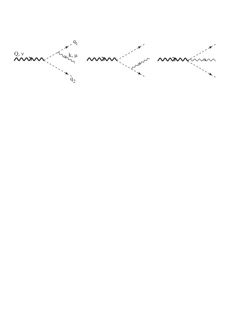
Figure 1: Diagrams for the $\rho^{0}\rightarrow\pi^{+}\pi^{-}\gamma$ decay.

III.2.2 $a_{1}^{+}\rightarrow\pi^{+}\gamma$ decay

Next we consider the EM decay $a_{1}^{+}(Q)\rightarrow\pi^{+}(p)+\,\gamma(q).$  There is no contribution to the matrix element on the tree level, and we have to include at least the one-loop processes shown in Fig. 2 (see also Table 1).

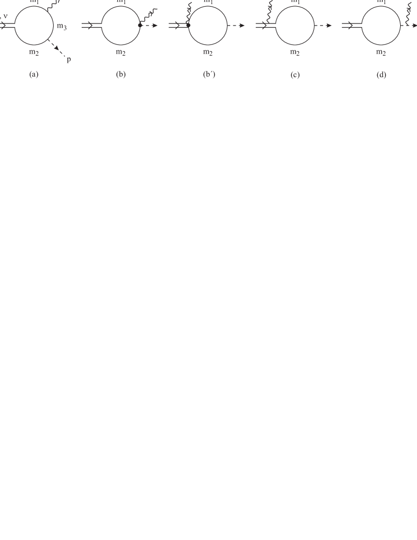
Figure 2: Diagrams for $a^{+}\rightarrow\pi^{+}\gamma$ decay at the one-loop level. The intermediate propagators labeled $m_{1}$, $m_{2}$, $m_{3}$ refer to particles as defined in Table 1. Depending on the intermediate state $j$, the contact diagrams have the structure $(b)$ for $j=1,2,4,6,7$ and the structure $(b^{\prime})$ for $j=3,5,9,10$. For $j=8$ there is no contact diagram.

Table 1: Intermediate particles in the loop diagrams indicated in Fig. 2.

$j$	1	2	3	4	5	6	7	8	9	10
$m_{1}$	$\pi$	$\rho$	$\pi$	$a$	$\pi$	$a$	$\rho$	$N$	$\rho$	$a$
$m_{2}$	$\rho$	$\pi$	$\sigma$	$\sigma$	$\eta$	$\eta$	$\zeta$	$N$	$a$	$\rho$
$m_{3}$	$\pi$	$\rho$	$\pi$	$a$	$\pi$	$a$	$\rho$	$N$	$\rho$	$a$

These contributions can be obtained by attaching the photon line to the lines of the charged particles in the mixed self-energy operator $\Sigma_{a\pi}(Q),$ and by adding diagrams coming from the contact terms in the current (40). Each one-loop diagram for $\Sigma_{a\pi}(Q)$ gives rise to four diagrams [labeled (a),(b),(c),(d) in Fig. 2] for the EM process. The amplitude can be written as a sum

$$\mathcal{M=}\sum_{j=1}^{10}\mathcal{M}_{j}=\sum_{j=1}^{10}\epsilon_{\nu}(a)\epsilon_{\mu}^{\ast}(\gamma)\ M_{j}^{\mu\nu},$$ (52)

where $j$ labels the intermediate state in the loop, namely $j=(\pi^{+}\rho^{0})$, $(\pi^{0}\rho^{+})$, $(\pi^{+}\sigma)$, $(a^{+}\sigma)$, $(\pi^{+}\eta)$, $(a^{+}\eta)$, $(\rho^{+}\zeta)$, $(p\bar{n})$, $(\rho^{+}a^{0})$, and $(\rho^{0}a^{+})$. Note that in the present study, because of the technical complexity, the diagrams with $j=9$ and $j=10$ (containing at least two vector or axial-vector propagators in the loop) are not included. Calculation of the amplitudes is cumbersome and we refer to Appendix B for details. However, some features of the calculation are worth mentioning here.

i) Each amplitude $M_{j}^{\mu\nu}$ is gauge invariant and has the structure

$$M_{j}^{\mu\nu}=(g^{\mu\nu}-\frac{Q^{\mu}q^{\nu}}{Q\cdot q})\,T_{j},$$ (53)

where the $T_{j}$ are Lorentz scalars. This serves as an important check of the calculation. The contact terms $\gamma\pi\pi\rho,\gamma\pi\sigma a,\gamma\rho aa,\gamma\pi a\eta$  and $\gamma\pi\rho\zeta$ in Eq.(40) are crucial to ensure this property.

ii) The diagrams with the bremsstrahlung from the final pion [labeled (d) in Fig. 2] do not contribute to the matrix element for the on-mass-shell $a_{1}$ meson. Indeed, the polarization vector of the $a_{1}$ meson satisfies the relation  $\epsilon(a)\cdot Q=0.$  It is easy to check that the matrix element corresponding to these diagrams is in each case proportional to $Q^{\nu},$ and therefore vanishes when multiplied by $\epsilon_{\nu}(a).$

iii) Some of the diagrams on Fig. 2 are divergent. However, the divergent terms from the different diagrams in any $M_{j}^{\mu\nu}$ cancel, and the total amplitude is finite. The calculations are done in the unitary gauge using the method of dimensional regularization (see Appendix B), in which the cancellation of divergencies is explicitly verified.

iv) The diagrams with $j=5,6,7$ in Fig. 2 contain intermediate Higgs mesons $\eta$ and $\zeta$. If one takes the mass $m_{H}$ of these mesons very large the amplitudes remain finite and correspond to a contact-like $\gamma\pi a$ Lagrangian

$$\mathcal{L}_{cont}(\gamma\pi a)=h(\partial_{\mu}A_{\nu}-\partial_{\nu}A_{\mu})(\mbox{\boldmath$\pi$\unboldmath}\times\partial^{\mu}\mathbf{a}^{\nu})_{3}$$ (54)

where  $h=-(4\pi)^{-2}eg_{\rho}^{2}(1-X_{\pi})^{1/2}/(3m_{\rho}).$

v) The amplitudes $M_{j}^{\mu\nu}$ for $j=1,2,3$ have both real and imaginary parts, because the masses of the intermediate particles in these diagrams satisfy the condition $m_{1}+m_{2}<m_{a}$.  The amplitudes  $M_{j}^{\mu\nu}$ for $j=4,...,10$ are real.

vi) The most complicated diagrams are those involving the EM vertex of the $\rho$ and $a_{1}$ mesons. The vertex for the $\gamma\rho\rho$ (or $\gamma aa)$ has the form

$$\Gamma^{\mu\nu\lambda}(q,r,p) = e\{g^{\lambda\nu}(r-p)^{\mu}-g^{\mu\nu}r^{\lambda}+g^{\lambda\mu}p^{\nu}+(g^{\mu\nu}q^{\lambda}-g^{\mu\lambda}q^{\nu})\}\delta^{ij}$$ (55)

$$= e\{g^{\lambda\nu}(r-p)^{\mu}+g^{\mu\nu}(q-r)^{\lambda}+g^{\lambda\mu}(p-q)^{\nu}\}\delta^{ij},$$

where $q$ is the momentum of the photon (with the Lorentz index $\mu),$ $p$ and $r$ are the momenta of the $\rho$ (with the Lorentz indices $\lambda$ and $\nu$), and $p+q+r=0$. In the first line we explicitly separated the minimal EM interaction and coupling to the intrinsic magnetic moment of the mesons.

vii) In the rest frame of the meson $a_{1},$ where $Q^{\nu}=(m_{a,}\mathbf{0}),$ one can use the additional relation $Q\cdot\epsilon(\gamma)=0$, as the photon polarization vectors have only space-like components. Therefore in the general structure of the amplitude of Eq.(53), only the term proportional to $g^{\mu\nu}$ contributes.

The width of the $a_{1}^{+}\rightarrow\pi^{+}\gamma$ decay is expressed in terms of the $T_{j}$ as follows

$$\Gamma=\frac{|\mathbf{p}|}{8\pi m_{a}^{2}}\frac{2}{3}\,\left|\sum_{j=1}^{10}T_{j}\right|^{2}.$$ (56)

The results of the calculation are presented in Table 2.

Table 2: Contribution of different diagrams on Fig. 2 to the $a^{+}\to\pi^{+}\gamma$ decay width. Values are given in KeV.

Intermediate state in the diagrams	$m_{a}=1.23$ GeV	$m_{a}=1.089$ GeV	Experiment PDG
$\pi^{+}\rho^{0}$	469	330
$\pi^{+}\rho^{0}+\pi^{0}\rho^{+}$	187	89
$\pi^{+}\rho^{0}+\pi^{0}\rho^{+}+\pi^{+}\sigma$	211	104
$\pi^{+}\rho^{0}+\pi^{0}\rho^{+}+\pi^{+}\sigma+a^{+}\sigma$	845	434
$\pi^{+}\rho^{0}+\pi^{0}\rho^{+}+\pi^{+}\sigma+a^{+}\sigma$+
$\;\;\;\;\;\;\;\;\;\;\;\;+\ [\pi^{+}\eta+a^{+}\eta+\rho^{+}\zeta]$	646	345
$\pi^{+}\rho^{0}+\pi^{0}\rho^{+}+\pi^{+}\sigma+a^{+}\sigma+$
$\;\;\;\;\;\;\;\;\;\;\;\;+\ [\pi^{+}\eta+a^{+}\eta+\rho^{+}\zeta]+p\bar{n}$	412	192	640$\pm 246$

Calculations were performed with two values of the $a_{1}$-meson mass: 1.23 GeV PDG , and $\sqrt{2}m_{\rho}=1.089$ GeV. The latter value is often discussed in the literature Gil68 ; Mei88 ; Wei90 . One notices from Table 2 that the different amplitudes strongly interfere. For example, the $\pi^{+}\rho^{0}$ and $\pi^{0}\rho^{+}$ amplitudes almost cancel each other. A substantial contribution comes from the $a^{+}\sigma$ loop ($j=4)$, due to the large value of the constant in front of the integral. There is a dependence on the $\sigma$ mass, but it is weak. We used here $m_{\sigma}=770$ MeV. The diagrams in Fig. 2 containing the intermediate Higgs mesons give a relatively small contribution, as can be seen from the sixth row in Table 2. The $N\bar{N}$ diagrams ($j=8)$ by themselves would give a small contribution. However, due to the interference with other diagrams, their effect becomes sizeable. On the whole, the calculation with $m_{a}=1.23$ GeV yields a width in agreement with experiment. Note however that the diagrams with $j=9$ and $j=10$ were not included.

III.2.3 $\rho^{+}\rightarrow\pi^{+}\gamma$  decay

The diagram contributing to the $\rho^{+}(Q)\rightarrow\pi^{+}(p)+\gamma(q)$ decay on the one-loop level is shown in Fig. 3. The matrix element for this process, like for any anomalous decay, has the structure Pes95 (Ch.19.3): $\mathcal{M}=\varepsilon^{\mu\nu\lambda\sigma}\epsilon_{\mu}^{\ast}(\gamma)\epsilon_{\nu}(\rho)Q_{\lambda}q_{\sigma}/(Q\cdot q)\,T,$ where $\varepsilon^{\mu\nu\lambda\sigma}$ is the Levi-Civita antisymmetric tensor, and $T$ depends on the coupling constants and masses of the particles. The one-loop integral corresponding to Fig. 3 converges, and using standard methods we obtain (see Appendix B)

$$T=(4\pi)^{-2}2eg_{\rho}g_{\pi}m_{N}\sqrt{X_{\pi}}\int_{0}^{1}\log\left[\frac{m_{N}^{2}-m_{\rho}^{2}x(1-x)}{m_{N}^{2}-m_{\pi}^{2}x(1-x)}\right]\frac{\mbox{\rm d}x}{1-x}.$$ (57)

The calculated decay width is 55 KeV, while the PDG PDG quotes the value 68$\pm 7$ KeV. In view of the simple mechanism assumed for this decay we consider the agreement between the calculation and experiment satisfactory . It is worthwhile to mention that the factor $g_{\pi}g_{\rho}\sqrt{X_{\pi}},$ which defines the magnitude of the matrix element, is considerably smaller than one would get using the conventional values for the couplings. For example, with the typical values $g_{\pi}=13.0,$ $g_{\rho}=6.04$ (and $X_{\pi}=1$) the width would increase to 160 KeV.

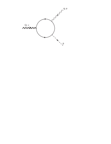
Figure 3: One-loop diagram corresponding to $\rho^{+}\rightarrow\pi^{+}\gamma$ decay.

All calculated decay widths are collected in Table 3, where they are compared with experimental values PDG . We also included in Table 3 the results Ko94 obtained in a version of GLSM with massive $\rho$ and $a_{1}$ mesons, where several additional terms were introduced. In particular, the $a_{1}^{+}\rightarrow\pi^{+}\gamma$ decay in Ko94 appears on the tree level due to the introduction of dimension-6 operators in the Lagrangian. Some results in the non-linear realization of the chiral symmetry (hidden symmetry approach) from ref. Mei88 (Ch.3) are shown in the 7th column.

Table 3: Widths of strong and electromagnetic decay of mesons. Calculations are performed with two masses of the $\sigma$ meson: $m_{\sigma}^{(a)}=770$ MeV and $m_{\sigma}^{(b)}=1$ GeV. Experimental values are from PDG .

Meson decay	$m_{a}=1.230$ GeV		$m_{a}=1.089$ GeV		Ref. Ko94	Ref. Mei88	Experiment
	$m_{\sigma}^{(a)}$	$m_{\sigma}^{(b)}$	$m_{\sigma}^{(a)}$	$m_{\sigma}^{(b)}$
$a_{1}\rightarrow\pi\rho$ [MeV]	272	272	163	163	483	360	150 to 361
$D/S$  ratio [%]	-4.6	-4.6	-2.3	-2.3	7.8		-10.7$\pm 1.6$
$a_{1}\rightarrow\pi\sigma$ [MeV]	46	4.7	21	-			32 to 147
$\Gamma(a_{1}\rightarrow\pi\sigma)/\Gamma_{tot}$ [%]	$\approx$ 14	$\approx$ 1.7	$\approx$ 11	-			18.76$\pm 4.29\pm$1.48
$\sigma\rightarrow\pi\pi$ [MeV]	149	346	325	753	373
$\rho^{0}\rightarrow\pi^{+}\pi^{-}\gamma$ [MeV]:
$\;\;\;(k_{\min}=50$ MeV)	1.73	1.73	1.73	1.73			1.487$\pm 0.240$
$\;\;\;(k_{\min}=60$ MeV)	1.49	1.49	1.49	1.49
$a_{1}^{+}\rightarrow\pi^{+}\gamma$ [KeV]	412	411	192	180	670	300	640$\pm 246$
$\rho^{+}\rightarrow\pi^{+}\gamma$ [KeV]	55	55	81	81		80	68 $\pm 7$

IV $\pi-\pi$ scattering at low energies

Pion-pion scattering is a process where one can test the strong-interaction Lagrangian. Let us first analyze the terms in the Lagrangian in Eqs.(42) and (43) which are relevant for the $\pi-\pi$ scattering on the tree level:

$$\Delta\mathcal{L} = -\lambda X_{\pi}\mbox{\boldmath$\pi$\unboldmath}^{2}(v\sigma+\frac{1}{4}X_{\pi}\mbox{\boldmath$\pi$\unboldmath}^{2})-\frac{1}{2}g_{\rho}(1+X_{\pi})\mbox{\boldmath$\rho$\unboldmath}_{\mu}(\mbox{\boldmath$\pi$\unboldmath}\times\partial^{\mu}\mbox{\boldmath$\pi$\unboldmath})$$ (58)

$$-\frac{\lambda_{H}}{8}(1-X_{\pi})\mbox{\boldmath$\pi$\unboldmath}^{2}[u\eta+\frac{1}{4}(1-X_{\pi})\mbox{\boldmath$\pi$\unboldmath}^{2}].$$

This Lagrangian has several unusual features. Firstly, the $\sigma\pi\pi$ interaction and the related $\pi^{4}$ interaction, coming from the first term in Eq.(58), are suppressed by the factors $X_{\pi}$ and  $X_{\pi}^{2}$ respectively. This will lead to a suppression of the corresponding amplitude by the factor $X_{\pi}^{2}\approx 0.15.$ Secondly, the $\rho$-meson exchange is determined by the coupling $g_{\rho\pi\pi}=g_{\rho}(1+X_{\pi})/2$ which is fixed from the $\rho\rightarrow\pi\pi$ decay. Thirdly, the last term, containing $\eta\pi\pi$ and $\pi^{4}$ interactions, has a coupling $\lambda_{H}$ which rises with the Higgs mass $m_{H}$ (see Eq.(22)). At first sight this leads to a divergence of the tree-level amplitude in the limit $m_{H}\rightarrow\infty$, and it seems unlikely that the Lagrangian (58) can give reasonable predictions for $\pi-\pi$ scattering. In this section we will study this issue by calculating the low-energy scattering parameters for the $S-$ and $P-$waves.

The formalism of $\pi-\pi$ scattering has been considered in many references (see, e.g. Ber91 ; Ko94 ), and we briefly recall the basic relations. The scattering amplitude for the reaction  $\pi^{i}+\pi^{j}\rightarrow\pi^{k}+\pi^{l}$  can be written as

$$\mathcal{M}_{ij,kl}=M(s,t,u)\delta^{ij}\delta^{kl}+M(t,s,u)\delta^{ik}\delta^{jl}+M(u,t,s)\delta^{il}\delta^{jk},$$ (59)

where $i,j,k,l$ label the charge states of the pions, and $s,t,u$ are the conventional Mandelstam variables. One also defines the amplitudes $M^{(I)}$  with total isospin $I=0,1,2:$

$$M^{(0)} = 3M(s,t,u)+M^{(2)},\,\ \ \ \ \ \ \ \ \ \ \ \ \ \ \ \ M^{(1)}=M(t,s,u)-M(u,t,s),$$

$$M^{(2)} = M(t,s,u)+M(u,t,s).$$ (60)

The amplitude in a channel with fixed isospin is expanded in partial waves,

$$M^{(I)}=32\pi\sum_{l=0}^{\infty}(2l+1)P_{l}(\cos\theta)t_{l}^{(I)}(s),$$ (61)

where $P_{l}(\cos\theta)$ is the Legendre polynomial  and $\theta$ is the scattering angle. The partial-wave amplitude $t_{l}^{(I)}(s)$ can be approximated at small center-of-mass (CM) momentum $\mathbf{|q|}=(s/4-m_{\pi}^{2})^{1/2}$  as follows,

$$\mbox{\rm Re}\ t_{l}^{(I)}(s)\approx\frac{\mathbf{q}^{2l}}{m_{\pi}^{2l}}[a_{l}^{(I)}+b_{l}^{(I)}\frac{\mathbf{q}^{2}}{m_{\pi}^{2}}+\mathcal{O}(\frac{\mathbf{q}^{4}}{m_{\pi}^{4}})].$$ (62)

In order to find the scattering lengths $a_{l}^{(I)}$ and effective ranges$\ b_{l}^{(I)}$ one has to expand the amplitudes in Eq.(60) around $\mathbf{q}^{2}=0$, using the definition of the invariants in the CM frame

$$s=4(m_{\pi}^{2}+\mathbf{q}^{2}),\,\ \ \ \ \ \ \ \ \ \ \ \ \ \ \ \ \ \ t=-2\mathbf{q}^{2}(1-\cos\theta),\,\ \ \ \ \ \ \ \ \ \ \ \ \ \ \ \ u=-2\mathbf{q}^{2}(1+\cos\theta).$$ (63)

We now show that the Higgs part of the Lagrangian (last term in Eq.(58)) gives a finite contribution to $M(s,t,u)$. The $\eta$ exchange and $\pi^{4}$ interaction lead to the amplitude

$$M_{\eta}(s,t,u)=\left(-\frac{\lambda_{H}}{4}+\frac{1}{16}\frac{\lambda_{H}^{2}u^{2}}{m_{H}^{2}-s}\right)(1-X_{\pi})^{2}=\frac{g_{\rho}^{2}(1-X_{\pi})^{2}}{4m_{\rho}^{2}}\frac{s}{(1-s/m_{H}^{2})},$$ (64)

where we made use of $\lambda_{H}u^{2}=4m_{H}^{2}$, which follows from Eqs.(22). It is clear that the couplings in the $\eta$ exchange and the contact $\pi^{4}$ diagram are tuned in such a way that the sum remains finite at large $m_{H}.$

It is straightforward to obtain from Eq.(58) the amplitudes corresponding to $\sigma$ exchange, with the associated $\pi^{4}$ term, and $\rho$ exchange,

$$M_{\sigma}(s,t,u)+M_{\rho}(s,t,u)=-2\lambda X_{\pi}^{2}\frac{m_{\pi}^{2}-s}{m_{\sigma}^{2}-s}+g_{\rho\pi\pi}^{2}\left(\frac{s-u}{m_{\rho}^{2}-t}+\frac{s-t}{m_{\rho}^{2}-u}\right).$$ (65)

The total amplitude is $\ M(s,t,u)=$ $M_{\eta}(s,t,u)+M_{\sigma}(s,t,u)+M_{\rho}(s,t,u).$ The other amplitudes in Eq.(59) are obtained by interchanging $t\longleftrightarrow s,$ or $u\longleftrightarrow s.$ As expected, the $\sigma$ contribution in Eq.(65) is multiplied by $X_{\pi}^{2}$ which strongly reduces the effect of the $\sigma$ meson in $\pi-\pi$ scattering. The low-energy parameters can be found by expanding Eq.(64) and (65) in powers of $\mathbf{q}^{2}$, using the definitions (61),(63), and comparing the results with Eq.(62). The calculated coefficients $a_{l}^{(I)}$ and $b_{l}^{(I)}$ are presented in Table 4.

Table 4: Low-energy parameters for $\pi-\pi$ scattering. The $\sigma$-meson mass is 770 MeV, and the $a_{1}$-meson mass is 1.23 GeV.

Model	$a_{0}^{(0)}$	$b_{0}^{(0)}$	$a_{0}^{(2)}$	$b_{0}^{(2)}$	$a_{1}^{(1)}$
Present model: $\sigma$ + $\rho$ + $\eta$	0.238	0.319	-0.100	-0.155	0.061
–               only $\sigma$ + $\rho$	0.210	0.301	-0.100	-0.146	0.057
–               only $\rho$	0.191	0.273	-0.095	-0.137	0.055
– with form factor for $\rho$ exchange	0.160	0.200	-0.061	-0.097	0.040
($\Lambda=1.6$ GeV)
Soft-pion amplitude Wei66	0.159	0.182	-0.045	-0.091	0.030
ChPT (only pions)  Gae83	0.20	0.24	-0.042	-0.075	0.037
ChPT (pions and resonances) Ber91	0.21		-0.043		0.038
Experiment  Nag79 ; Rig91	0.26$\pm 0.05$	0.25$\pm 0.03$	-0.028$\pm 0.012$	-0.082$\pm 0.008$	0.038$\pm 0.002$
Experiment  Sev92	0.20$\pm 0.01$		-0.037$\pm 0.004$

It is seen from Table 4 that the scattering length $a_{0}^{(0)}$ is described fairly well. The other parameters, however, are overpredicted by a factor of 1.5$\div$2. The $\rho$ meson gives the dominant contribution (compare the 2nd and 4th rows), while the contribution of the Higgs meson is small (see the 2nd and 3d rows). In the 6th row we show parameters obtained with the soft-pion amplitude  $M_{SPA}(s,t,u)=(s-m_{\pi}^{2})\,/f_{\pi}^{2}$  from ref. Wei66 , which is based on PCAC and current commutation relations. Our amplitude will reduce to $M_{SPA}(s,t,u)$ if $\ g_{\rho}=0$ and  $m_{\sigma}^{2}\gg m_{\pi}^{2}.$  We also show results of the ChPT calculations: Gae83 , where only pions are included and Ber91 , where resonances are added.

Comparison with the experiment indicates that the effect of the $\rho$ meson is overemphasized in the present model. In this connection we compare the $\rho$-exchange amplitude in Eq.(65) with the corresponding amplitude by Bernard et al. [Eq.(3.14) in ref. Ber91 ]. One of the differences is that in Ber91 the propagator of the vector meson (to be exact, the part contributing for on-shell pions) is modified according to

$$\frac{1}{m_{\rho}^{2}-t}\longrightarrow\frac{t}{m_{\rho}^{2}(m_{\rho}^{2}-t)}=\frac{1}{m_{\rho}^{2}-t}-\frac{1}{m_{\rho}^{2}},$$ (66)

which coincides with Weinberg’s suggestion Wein68 based on chiral-symmetry arguments. Such a modification strongly reduces the effect of the $\rho$ meson at low energies. In the present model however there is no compensating term of the form Wein68  $\sim(\mbox{\boldmath$\pi$\unboldmath}\times\partial_{\mu}\mbox{\boldmath$\pi$\unboldmath})^{2}$ which would lead to Eq.(66). Using the $\pi\pi\rho$ interaction with more derivatives, as is advocated in ref. Ber91 , would also be inconsistent with the Lagrangian (42). Besides, the calculation shows that the effect of the $\rho$ meson cannot be eliminated completely as would follow from Eq.(66), since the $\sigma$ contribution in itself is by far too small. One of the mechanisms which can partly reduce the $\rho$ contribution is the dependence of the $\rho\pi\pi$ vertex on the invariant mass of the $\rho.$ One may assume that $\ g_{\rho\pi\pi}(t)=g_{\rho\pi\pi}F_{\rho\pi\pi}(t)$  with a form factor normalized to unity at $t=m_{\rho}^{2}.$ The typical form often used in phenomenological models is  $F_{\rho\pi\pi}(t)=(\Lambda^{2}-m_{\rho}^{2})/(\Lambda^{2}-t),$ where $\Lambda$ is a cut-off parameter. Choosing the value $\Lambda=1.6$ GeV Loh90 we obtain a considerable reduction of the low-energy parameters (see Table 4, the 5th row). Of course this is only one plausible argument which may explain the unsatisfactory description of low-energy $\pi-\pi$ scattering on the tree level. Besides the form factor, other higher-order corrections to the amplitude would have to be consistently included. This issue will be studied elsewhere.

V Discussion and conclusions

In the previous sections we have presented the results of calculations in the framework of a new representation of QHD-III Pre99 . An advantage of this new form, compared to the original formulation Ser92 , is that only simple vertices with at most one derivative appear in the Lagrangian. As a result the calculations are simpler, and more importantly, the strong-interaction vertices describing the decay of the mesons do not vanish at any values of the meson invariant mass. A comparison with experiment (Table 3) shows that most of the decay widths are reasonably described. This was not anticipated in view of the fact that practically no free parameters were used in the calculations. In fact, only the coupling $g_{\rho}$ was fixed from the $\rho\rightarrow\pi\pi$ decay. The masses of the nucleon, pion, rho and $a_{1}$ mesons were taken from the latest PDG review PDG .

The mass of the $\sigma$ meson was chosen equal to the mass of the $\rho,$ i.e. $m_{\sigma}=m_{\rho}=770$ MeV, in line with ref. Wei90 where the $\sigma$ is supposed to be degenerate with the $\rho$. With this mass the calculated width for the $a_{1}\rightarrow\pi\sigma$ decay, 46 MeV, is surprisingly close to the value predicted in Wei90 : $\Gamma(a_{1}\rightarrow\pi\sigma)=\Gamma(\rho\rightarrow\pi\pi)\,/\sqrt{8}\approx 50$ MeV. In some calculations we use the value $m_{\sigma}=$ 1 GeV. As a result the widths of the $a_{1}\rightarrow\pi\sigma$ and $\sigma\rightarrow\pi\pi$ decays change considerably due to a change of the available phase space. The other observables are not sensitive to the $\sigma$ mass. Calculations were also performed with the value $m_{a}=\sqrt{2}m_{\rho}=1.089$ GeV, which is based on different arguments Gil68 ; Wei90 . However, agreement with experiment is better with the PDG value $m_{a}=1.23$ GeV. As a curious observation we mention that this value approximately obeys the relation $m_{a}\approx(1+\sqrt{2})^{1/2}m_{\rho}$ within a 3% accuracy. This relation also implies that $g_{\rho}/g_{\rho\pi\pi}=2m_{a}^{2}/(m_{a}^{2}+m_{\rho}^{2}),$ i.e. the ratio of the $\rho$ couplings to the nucleon and the pion, is very close to $\sqrt{2}.$

The EM decay $\rho^{0}\rightarrow\pi^{+}\pi^{-}\gamma$ is described by the two-step tree-level amplitude supplemented by a contact diagram. The latter comes from the  $\gamma\pi\pi\rho$ vertex in the EM current (39) and guarantees the EM gauge invariance. The decay is mainly determined by the $\rho\pi\pi$ coupling and is not sensitive to other ingredients of the model. The decay $a_{1}^{+}\rightarrow\pi^{+}\gamma$ is a more informative process. As there is no direct $a\pi\gamma$ coupling the process is described by many one-loop diagrams which strongly interfere. The total amplitude of $a_{1}^{+}\rightarrow\pi^{+}\gamma$ comes out finite despite the divergence of the separate diagrams. Since the Lagrangian was obtained in the unitary gauge, the propagator of the vector mesons includes the longitudinal component $k^{\mu}k^{\nu}/m^{2}.$ The latter gives rise to a quadratic divergence, $\sim\Gamma(1-d/2)$, but due to the EM gauge invariance these divergences from different diagrams cancel. Furthermore, the logarithmic divergences, $\sim\Gamma(2-d/2)$, cancel as well.

The Higgs mesons, $\eta$ and $\zeta$, play the role of auxiliary particles in this model. According to ref. Ser92 these mesons serve as regulators and should have minimal effect on the low-energy predictions. They do not appear in the initial and final states, but may contribute as intermediate particles. For instance, the $\eta$ and $\zeta$ appear in one-loop diagrams for the $a_{1}^{+}\rightarrow\pi^{+}\gamma$ decay. In the diagrams with intermediate $\pi^{+}\eta$ state, the $\pi\pi\eta$ coupling in Eq.(43) increases proportionally to $m^{2}_{H}.$ However, due to the presence of the $\eta$ propagator this contribution stays finite. The situation is different in the diagrams with an intermediate $a^{+}\eta$ and $\rho^{+}\zeta$, where the vertices $aa\eta$ and $a\rho\zeta$ are independent of $m_{H}$. Nevertheless the amplitudes do not vanish in the limit $m_{H}\rightarrow\infty$, as one would naively expect by taking the limit of the propagator in the loop integrand. This is because the longitudinal component of the vector meson propagator leads to divergent integrals; the correct procedure is to take the limit $m_{H}\rightarrow\infty$ after the loop integration, and leads to a nonzero contribution. At $m_{H}\rightarrow\infty$ the total amplitude corresponding to the above processes involving Higgs mesons takes a form equivalent to an effective $a\pi\gamma$ Lagrangian. Numerically its contribution to the $a_{1}^{+}\rightarrow\pi^{+}\gamma$ decay turns out to be relatively small.

In processes where $\eta$ and $\zeta$ appear on the tree level the amplitude may diverge at $m_{H}\rightarrow\infty$, if there are more $\pi\pi\eta$ vertices than the $\eta$ propagators. Using the $\pi-\pi$ scattering as an example we demonstrated that this is not the case. In this reaction there is the $\eta$-exchange diagram which at first sight behaves as $m_{H}^{2}$. However there is a compensating $\pi^{4}$ vertex in the Lagrangian (43). The couplings in the $\eta$ exchange and $\pi^{4}$ contact diagrams are tuned in such a way that the sum remains finite. This mechanism of cancellation is similar to that in the linear sigma model, in which the amplitude given by the $\sigma$ exchange and the $\pi^{4}$ vertex does not diverge in the limit $m_{\sigma}\rightarrow\infty$, but rather takes the value dictated by the soft-pion amplitude Wei66 . The contribution of the $\eta$ exchange and the associated $\pi^{4}$ term at low energies is small.

The pion interaction with hadrons in the model is scaled down by the factor $\sqrt{X_{\pi}}=m_{\rho}/m_{a}$ (with the exception of the $\pi\pi\rho$, $\pi\pi\rho\rho$ and $\pi\pi aa$ vertices). This influences the matrix elements of the meson decays, and in most cases improves agreement with experiment. The factor $m_{\rho}/m_{a}$ also leads to a reduction of the $\sigma\rightarrow\pi\pi$ decay width. For example, compared to the linear sigma model the width is reduced by almost an order of magnitude. Therefore the width comes out smaller than the $\sigma$ mass [of the order of 150 (350) MeV for $m_{\sigma}=$0.77 (1.0) GeV] which may be helpful in identifying the $\sigma$ with the scalar-isoscalar state around 1 GeV PDG . At the same time the effect of the $\sigma$ in $\pi-\pi$ scattering is also diminished. Our calculation shows that the $\sigma$ contribution to the low-energy parameters becomes very small, and the dominant contribution comes from the $\rho$ exchange. The agreement between the calculation and experiment is not very impressive compared to, for example, ChPT calculations. The scattering length in the $I=0,\ l=0$ channel is described quite well, but the other calculated parameters overestimate the experiment. This deficiency may be related to the tree-level approximation. We included a form factor in the $\pi\pi\rho$ vertex, similarly to what is often done in phenomenological models. This is one of the effects which contribute beyond the tree level. In this way the $\rho$ contribution is reduced and the agreement is improved, but other higher-order corrections need to be consistently taken into account before definite conclusions can be drawn.

In this paper we focused on the meson properties and left out the nucleon sector. Inclusion of the latter can also be an important test of the model, especially because the nucleon-pion vertex is reduced. At this point we would like to mention that we did not include an additional baryon, the cascade $\Xi=(\Xi^{0},\Xi^{-})$ with the hypercharge $Y_{\Xi}=-1$. This isodoublet was added in Ser92 to cure the problem with the chiral anomaly and render the theory renormalizable. The chiral anomaly in QHD-III will show up when the isoscalar $\omega$ meson couples to the baryon loop with other two isovector vertices, one of which contains $\gamma_{5}$. Such processes were not considered here. The anomaly may however be important in the EM decay $\rho^{+}\rightarrow\pi^{+}\gamma$ considered in Sect. III.2.3. If we added the loop with the cascade then the calculated width would change, though we did not include this effect. It seems logical first to extend the $SU(2)_{R}\times SU(2)_{L}$ model to the strange sector, as for example, was done in ref. Gas69 for GLSM. The extension to $SU(3)_{R}\times SU(3)_{L}$ would allow one to include along with $\Xi$ the other strange hadrons, like $\Lambda,\Sigma$ and $K.$

In conclusion, we applied chiral quantum hadrodynamics (QHD-III) Ser92 in the calculation of some properties of the mesons. First we included electromagnetic interaction by extending the symmetry to the local $U(1)\times SU(2)_{R}\times SU(2)_{L}$ group. This allowed us to obtain consistently the minimal and nonminimal contributions to the electromagnetic interaction in an arbitrary gauge. After an appropriate diagonalization and fixing the gauge the Lagrangian is obtained in terms of the physical pion field. We calculated the strong and EM decays of the vector and axial-vector mesons, $a_{1}\rightarrow\pi\rho$, $a_{1}\rightarrow\pi\sigma$, $\rho^{0}\rightarrow\pi^{+}\pi^{-}\gamma$, $a_{1}^{+}\rightarrow\pi^{+}\gamma$, $\rho^{+}\rightarrow\pi^{+}\gamma$, and addressed the issue of the width of the $\sigma$ meson. For the $a_{1}^{+}\rightarrow\pi^{+}\gamma$ decay some loop diagrams are not yet included, and a more complete analysis is reserved for future work. Most of the calculated decay widths are in reasonable agreement with experiment PDG . The only free parameter used in calculations is the mass of the $\sigma$ meson, although most of the results were not sensitive to $m_{\sigma}.$

We studied the effect of auxiliary Higgs bosons of QHD-III in the $a_{1}^{+}\rightarrow\pi^{+}\gamma$ decay and $\pi-\pi$ scattering. The contribution of these particles to the amplitude, both on the tree level and in the one-loop diagrams, turns out to be finite and small in the limit $m_{H}\rightarrow\infty$. This goes in line with the viewpoint of ref. Ser92 on the role of $\eta$ and $\zeta$ mesons in low-energy hadron physics.

Our exploratory study shows that QHD-III in the representation of ref.Pre99 can describe some features of meson phenomenology in the non-strange sector. There are many interesting issues which can be further addressed, such as an extension of calculations to the baryon sector ($\pi-N$ scattering and nucleon form factors), a clarification of the role of the cascade $\Xi$ and inclusion of the other strange hadrons. Finally, applications to the many-body sector, i.e. nuclear matter and finite nuclei, may be considered. As was shown in ref. Fur93 (see also Ser97 , sect. 3A), the linear sigma model, when applied to finite nuclei on the mean-field level, has some deficiencies. The present model is much richer and differs in several respects, such as the presence of additional particles and vertices, and a considerable suppression of the pseudo-scalar pion-nucleon coupling. Detailed calculation will help to assess the applicability of the model to the many-body sector.

Appendix A Derivation of the Lagrangian in the Higgs sector in an arbitrary gauge

The most complicated part of the Higgs Lagrangian are the terms with the covariant derivatives. For the right field, for example, such a term can be written in the form

$$(D_{\mu}\Phi_{R})^{\dagger}(D^{\mu}\Phi_{R})=\frac{1}{4}\left(\begin{array}[]{cc}0&1\end{array}\right)[Y_{1}\cdot Y_{1}+Y_{2}\cdot Y_{2}+Y_{3}\cdot\tilde{Y}_{3}-Y_{1}\cdot(Y_{3}+\tilde{Y}_{3})+i(Y_{2}\cdot\tilde{Y}_{3}-Y_{3}\cdot Y_{2})]\left(\begin{array}[]{c}0\\ 1\end{array}\right)\,,$$ (67)

where the operators $Y_{1},Y_{2},Y_{3}$ and  $\tilde{Y}_{3}$ are defined as

$$Y_{1}^{\mu} = (\partial^{\mu}\eta+\partial^{\mu}\zeta),\;\;\;\;\;\;\;\;Y_{2}^{\mu}=\mbox{\boldmath$\tau$\unboldmath}(\partial^{\mu}\mathbf{H+\partial}^{\mu}\mathbf{Z})+\frac{1}{2}(u+\eta+\zeta)Y_{4}^{\mu},\;\;\;\;\;$$

$$Y_{3}^{\mu} = \frac{1}{2}\mbox{\boldmath$\tau$\unboldmath}(\mathbf{H+Z})Y_{4}^{\mu},\;\;\;\;\;\;\;\;\tilde{Y}_{3}^{\mu}=\frac{1}{2}Y_{4}^{\mu}\mbox{\boldmath$\tau$\unboldmath}(\mathbf{H+Z}),$$

$$Y_{4}^{\mu} = g^{\prime}_{\rho}\mbox{\boldmath$\tau$\unboldmath}(\mbox{\boldmath$\rho$\unboldmath}^{\prime\mu}+\mathbf{a}^{\mu})+e^{\prime}A^{\prime\mu}\approx g_{\rho}\mbox{\boldmath$\tau$\unboldmath}({\mbox{\boldmath$\rho$\unboldmath}}^{\mu}+\mathbf{a}^{\mu})+e{A}^{\mu}(1+\tau_{3}),$$ (68)

and the notation $X\cdot Y=X_{\mu}Y^{\mu}$ is used. The similar term for the field $\Phi_{L}$ can be obtained from the above formulas by changing  $\zeta\rightarrow-\zeta,$ $\mathbf{Z}\rightarrow-\mathbf{Z}$ and $\mathbf{a}_{\mu}\rightarrow-\mathbf{a}_{\mu}.$ The potential $V_{H}$ in Eq.(3) is chosen such that $\lambda_{H}>0$ and $\mu_{H}^{2}>0,$ thus allowing for SSB of the global gauge invariance Ser92 . From the condition that the term linear in $\eta$ must be absent, the VEV $u$ can be found. The fields $\eta$ and $\zeta$ acquire a mass $m_{H}$, whereas $\mathbf{H}$ and $\mathbf{Z}$ remain massless, indicating that these are the Goldstone bosons.

Calculation of the matrix elements in Eq.(67) leads to the EM current in Eq.(16) and (17). The strong Lagrangian consists of the free Lagrangians in Eqs.(20-21), the mixing term in Eq.(19), and the interaction Lagrangian

$$\mathcal{L}_{H}^{int} = \frac{1}{8}g_{\rho}^{2}\{(\mbox{\boldmath$\rho$\unboldmath}_{\mu}^{2}+\mathbf{a}_{\mu}^{2})(\eta^{2}+\zeta^{2}+\mathbf{H}^{2}+\mathbf{Z}^{2}+2u\eta)+4\mbox{\boldmath$\rho$\unboldmath}_{\mu}\mathbf{a}^{\mu}[(u+\eta)\zeta+\mathbf{HZ}]\}$$ (69)

$$+\frac{1}{2}g_{\rho}[\mbox{\boldmath$\rho$\unboldmath}_{\mu}(\eta\partial^{\mu}\mathbf{H}-\mathbf{H}\partial^{\mu}\eta+\zeta\partial^{\mu}\mathbf{Z}-\mathbf{Z}\partial^{\mu}\zeta-\mathbf{H}\times\partial^{\mu}\mathbf{H}-\mathbf{Z}\times\partial^{\mu}\mathbf{Z})+\mathbf{a}_{\mu}(\eta\partial^{\mu}\mathbf{Z}-\mathbf{Z}\partial^{\mu}\eta$$

$$+\zeta\partial^{\mu}\mathbf{H}-\mathbf{H}\partial^{\mu}\zeta-\mathbf{H}\times\partial^{\mu}\mathbf{Z}-\mathbf{Z}\times\partial^{\mu}\mathbf{H})]-v_{H}(\eta,\zeta,\mathbf{H,Z})\,,$$

where the remaining piece of the potential is

$$v_{H}(\eta,\zeta,\mathbf{H,Z}) = \frac{\lambda_{H}}{32}[\eta^{4}+\zeta^{4}+4u\eta^{3}+6\eta\zeta^{2}(2u+\eta)+\mathbf{H}^{4}+\mathbf{Z}^{4}+2\mathbf{H}^{2}\mathbf{Z}^{2}$$ (70)

$$+4(\mathbf{HZ})^{2}+2(\mathbf{H}^{2}+\mathbf{Z}^{2})(\eta^{2}+\zeta^{2}+2u\eta)+8(u+\eta)\zeta\mathbf{HZ}]\,.$$

Eqs.(69-70) will reduce to the Lagrangian of QHD-III Ser92 if we take $\mathbf{H}=\mathbf{Z}=0.$

The interaction Lagrangian of GLSM from Sect. II.2 follows from Eqs.(23) - (26) after we define the $\sigma$ field through $\phi=v+\sigma\$, where the VEV $v$ can be fixed from the minimum of the potential, $\lambda v^{3}-\mu^{2}v-c=0$. The Lagrangian has the form

$$\mathcal{L}_{N\pi\sigma\omega}^{int} = -\bar{N}[g_{\pi}(\sigma+i\gamma_{5}\mbox{\boldmath$\tau$\unboldmath}\mbox{\boldmath$\pi$\unboldmath})+g_{\rho}\gamma^{\mu}\frac{\mbox{\boldmath$\tau$\unboldmath}}{2}(\mbox{\boldmath$\rho$\unboldmath}_{\mu}+\gamma_{5}\mathbf{a}_{\mu})+g_{\omega}\gamma^{\mu}\omega_{\mu}]N$$ (71)

$$+g_{\rho}[\mathbf{a}_{\mu}(\mbox{\boldmath$\pi$\unboldmath}\partial^{\mu}\sigma-\sigma\partial^{\mu}\mbox{\boldmath$\pi$\unboldmath})-\mbox{\boldmath$\rho$\unboldmath}_{\mu}(\mbox{\boldmath$\pi$\unboldmath}\times\partial^{\mu}\mbox{\boldmath$\pi$\unboldmath})-g_{\rho}va_{\mu}(\mbox{\boldmath$\pi$\unboldmath}\times\mbox{\boldmath$\rho$\unboldmath}^{\mu}-\sigma\mathbf{a}^{\mu})]$$

$$+\frac{1}{2}g_{\rho}^{2}[(\mathbf{a}_{\mu}\mbox{\boldmath$\pi$\unboldmath})^{2}+(\mbox{\boldmath$\pi$\unboldmath}\times\mbox{\boldmath$\rho$\unboldmath}_{\mu}-\sigma\mathbf{a}_{\mu})^{2}]-\lambda(\sigma^{2}+\mbox{\boldmath$\pi$\unboldmath}^{2})[v\sigma+\frac{1}{4}(\sigma^{2}+\mbox{\boldmath$\pi$\unboldmath}^{2})]\,.$$

Appendix B Evaluation of loop integrals

Let us consider the amplitudes for $a_{1}^{+}\rightarrow\pi^{+}\gamma$ decay with an intermediate $(\pi^{+}\rho^{0})$ state, corresponding to diagrams in Fig. 2 with $j=1$. We introduce the following notation:

$$D_{k}=k^{2}-m_{\rho}^{2},\,\ \ \ \ \ \ \ \ \ \ \ d_{k+Q}=(k+Q)^{2}-m_{\pi}^{2},\,\ \ \ \ \ \ \ \ \ \ \ d_{k+p}=(k+p)^{2}-m_{\pi}^{2}$$ (72)

with $Q^{2}=m_{a}^{2},\,\ p^{2}=m_{\pi}^{2}$ and $\ q^{2}=0.$ The amplitude labeled $(a)$ in Fig. 2 has an integrand proportional to

$$M_{1a}^{\mu\nu} \Longrightarrow (2k+2Q-q)^{\mu}(2p+k)^{\sigma}(g_{\nu\sigma}-\frac{k_{\nu}k_{\sigma}}{m_{\rho}^{2}})\frac{1}{D_{k}\ d_{k+Q}\,d_{k+p}}$$ (73)

$$\Longrightarrow \frac{2(k+Q)^{\mu}}{D_{k}\ d_{k+Q}}\left[\frac{k^{\nu}}{m_{\rho}^{2}}-\frac{(2p+k)^{\nu}}{d_{k+p}}\right]\,.$$

The terms proportional to $Q^{\nu}$ and $q^{\mu}$ are omitted hereafter because of the relations $Q\cdot\epsilon(a)=0$ and $q\cdot\epsilon(\gamma)=0.$ The diagram $(b)$ in Fig. 2 has an integrand

$$M_{1b}^{\mu\nu}\Longrightarrow\frac{2}{D_{k}\ d_{k+Q}}\left(g^{\mu\nu}-\frac{k^{\mu}k^{\nu}}{m_{\rho}^{2}}\right).$$ (74)

For the diagram $(c)$ with photon bremsstrahlung off the $a_{1}$ meson we obtain after some algebra,

$$M_{1c}^{\mu\nu} \Longrightarrow \frac{1}{q\cdot Q\,D_{k}}\left[\frac{Q^{\mu}(k-2q)^{\nu}+(k+2Q)^{\mu}q^{\nu}-g^{\mu\nu}q\cdot(2Q+k)}{d_{k+p}}\right.$$ (75)

$$\left.-\frac{Q^{\mu}k^{\nu}+k^{\mu}q^{\nu}-g^{\mu\nu}q\cdot k}{m_{\rho}^{2}}\right].$$

Similarly we find for the diagram $(d)$ in Fig. 2 with bremsstrahlung off the pion,

$$M_{1d}^{\mu\nu}\Longrightarrow\frac{Q^{\mu}k^{\nu}}{D_{k}}\left(\frac{1}{q\cdot Q\,\,m_{\rho}^{2}\ }-\frac{1}{q\cdot Q\,\ d_{k+Q}}-\frac{2}{m_{\rho}^{2}\ d_{k+Q}}\right).$$ (76)

In the chosen unitary gauge the propagator of the vector meson includes three space-like polarization states. We notice that the most divergent terms proportional to $m_{\rho}^{-2}$, which come from the longitudinal component of the $\rho$ propagator, cancel. The term  $\sim(k^{\mu}q^{\nu}-g^{\mu\nu}q\cdot k)/D_{k}$ that remains in Eq.(75) is equal to zero after integration over $k$. Further, it is straightforward to check that the sum of the four diagrams does not depend on the photon gauge, i.e.  $q_{\mu}(M_{1a}^{\mu\nu}+M_{1b}^{\mu\nu}+M_{1c}^{\mu\nu}+M_{1d}^{\mu\nu})=0.$

To evaluate the integrals we apply the method of dimensional regularization (see, e.g. Pes95 , App.A). Using the Feynman parametrization and integrating over $k$ in $d$-dimensional space-time we obtain

$$M_{1}^{\mu\nu} = 2ifg^{\mu\nu}\frac{\Gamma(2-d/2)}{(4\pi)^{d/2}}\left\{-\frac{1}{2}\int_{0}^{1}\mbox{\rm d}u_{1}\int_{0}^{1-u_{1}}\mbox{\rm d}u_{2}\,\Delta_{1}^{d/2-2}\right.$$ (77)

$$\left.+\int_{0}^{1}\mbox{\rm d}u[\Delta_{2}^{d/2-2}-(1-\frac{u}{2})\,\Delta_{3}^{d/2-2}]\right\}\,,$$

where the constant $f$ reads $f=-ieg_{\rho}^{3}v\sqrt{X_{\pi}}(1+X_{\pi})/2$. The expressions for $\Delta_{1},\Delta_{2},\Delta_{3}$ will be specified below. We kept in Eq.(77) only the $g^{\mu\nu}$ part because of the condition $Q\cdot\epsilon(\gamma)=0$ (in the rest frame of $a_{1}$). Since the Gamma-function $\Gamma(2-d/2)$ has a pole at $d=4$ we have to verify that the expression in the curly brackets vanishes at $d=4.$ Using the expansions near $d=4$ Pes95 : $\ \Delta^{d/2-2}=1+(d/2-2)\log\Delta+\mathcal{O}((d/2-2)^{2})$ and  $\Gamma(2-d/2)=2/(4-d)-\gamma_{E}+\mathcal{O}(d/2-2)$,  we find that the pole term drops out because of the relation

$$-\frac{1}{2}\int_{0}^{1}\mbox{\rm d}u_{1}\int_{0}^{1-u_{1}}\mbox{\rm d}u_{2}\,+\int_{0}^{1}\mbox{\rm d}u[1-(1-\frac{u}{2})]=0\,.$$ (78)

The residue gives the amplitude

$$M_{1}^{\mu\nu}=ifg^{\mu\nu}(4\pi)^{-2}\left\{\int_{0}^{1}\int_{0}^{1}\log\,\Delta_{1}(x,y)\,\mbox{\rm d}x\mbox{\rm d}y+\int_{0}^{1}[(2-x)\,\log\Delta_{3}(x)-2\log\,\Delta_{2}(x)]\mbox{\rm d}x\right\},$$ (79)

where the integration variables $u_{1},\,u_{2}$ have been changed to $x,y$ defined such that $u_{1}=xy,\,\,u_{2}=x(1-y).$ In the above formulas $\gamma_{E}\approx 0.5772$ is the Euler-Mascheroni constant and

$$\Delta_{1}(x,y) = \Delta_{3}(x)-(m_{a}^{2}-m_{\pi}^{2})\,x(1-x)y,\;\;\;\;\;\;\;\;\Delta_{3}(x)=m_{\rho}^{2}(1-x)+m_{\pi}^{2}x^{2},\,$$

$$\Delta_{2}(x) = -m_{a}^{2}x(1-x)+m_{\rho}^{2}(1-x)+m_{\pi}^{2}x.$$ (80)

The argument of the logarithm can formally be made dimensionless by changing $\ \log\Delta_{i}\rightarrow\log(\Delta_{i}/\Lambda^{2}),$ where $\Lambda$ is a mass-scale parameter. This will not affect the amplitude, due to (78). Expression (79) can be further simplified by carrying out the integration over $y.$

The $N\bar{N}$-loop amplitudes [$j=8$ in Fig. 2] require a trace calculation, for example,

$$M_{8a}^{\mu\nu} \Longrightarrow \frac{\mbox{Tr}[(k/+p/+m_{N})\gamma^{\mu}(k/+Q/+m_{N})\gamma^{\nu}\gamma_{5}(k/+m_{N})\gamma_{5}]}{D_{k}\ D_{k+Q}D_{k+p}}$$ (81)

$$\Longrightarrow 4m_{N}\left[\frac{g^{\mu\nu}q\cdot(2k+Q)-(2k+Q)^{\mu}q^{\nu}}{D_{k}\ D_{k+Q}D_{k+p}}-\frac{g^{\mu\nu}}{D_{k}\ D_{k+p}}\right],$$

where $D_{k}=k^{2}-m_{N}^{2},\,\ D_{k+Q}=(k+Q)^{2}-m_{N}^{2},\,\$and$\ \ D_{k+p}=(k+p)^{2}-m_{N}^{2}$. The $(c)$ amplitude in Fig. 2 reads

$$M_{8c}^{\mu\nu}\Longrightarrow 4m_{N}\frac{g^{\mu\nu}}{D_{k}\ D_{k+p}}.$$ (82)

This amplitude cancels the divergent and EM gauge noninvariant piece of $M_{8a}^{\mu\nu}.$  Finally, the amplitude $M_{8d}^{\mu\nu}$ (radiation from the pion line) is zero, being proportional to $Q^{\nu}.$

An important observation is the cancellation of divergent terms between different diagrams. This, together with the EM gauge invariance, helps in evaluating the other diagrams in Fig. 2. Most of these diagrams are calculated similarly to $M_{1}^{\mu\nu}$ while others, where the photon couples to a vector meson in the loop, are more algebraically involved.

After this general consideration we present expressions for the amplitudes corresponding to the diagrams in Fig. 2 with $j=1,...,8$. For the $\pi-\rho$ loops ($j=1,2$) we obtain

$$T_{1} = C_{1}\{-\frac{1}{2}-\int_{0}^{1}\log\frac{\Delta_{2}(x)}{\Delta_{3}(x)}[2-x+\frac{\Delta_{3}(x)}{M^{2}(1-x)}]\ \mbox{\rm d}x\},$$ (83)

$$T_{2} = C_{2}\{\frac{1}{2}+\int_{0}^{1}\log\frac{\Delta_{2}(x)}{\Delta_{3}(x)}[x-3+\frac{1}{x}(\frac{\Delta_{3}(x)}{M^{2}}+2)]\ \mbox{\rm d}x\},$$ (84)

$$\Delta_{2}(x) = m_{\pi}^{2}x+m_{\rho}^{2}(1-x)-m_{a}^{2}x(1-x),\,\ \ \ \ \ \ \ \ \ \ \Delta_{3}(x)=m_{\pi}^{2}x^{2}+m_{\rho}^{2}(1-x),$$

$$C_{1} = C_{2}=(4\pi)^{-2}\frac{1}{2}eg_{\rho}^{3}v\sqrt{X_{\pi}}(1+X_{\pi}),$$

and we introduced the notation $M^{2}\equiv m_{a}^{2}-m_{\pi}^{2}=2Q\cdot q.$  Since  $m_{\pi}+m_{\rho}<m_{a}$  these amplitudes acquire an imaginary part if $\ \Delta_{2}(x)<0,$ and we have to select the proper branch of the logarithm. Recalling the prescription $\ m^{2}\rightarrow m^{2}-i0$  for the masses of the particles in the propagators, we have correspondingly $\ \Delta_{2}(x)\rightarrow\Delta_{2}(x)-i0$ and we can use the substitution

$$\log\Delta_{2}(x) = \log|\Delta_{2}(x)|-i\pi\theta(-\Delta_{2}(x))=\log|\Delta_{2}(x)|-i\pi\theta(x-x_{-})\theta(x_{+}-x),$$ (85)

$$x_{\pm} = \{(m_{a}^{2}+m_{\rho}^{2}-m_{\pi}^{2})\,\pm[(m_{a}^{2}+m_{\rho}^{2}-m_{\pi}^{2})^{2}-4m_{a}^{2}m_{\rho}^{2}]^{1/2}\}/2m_{a}^{2},$$

in Eq.(83) and (84) to calculate the real and imaginary parts. Here $\theta(y)=1$ if$\ y>0,$ and $0$ otherwise.

For the $j=3$ contribution we obtain

$$T_{3} = C_{3}\{-1+2\int_{0}^{1}\log\frac{\Delta_{2}(x)}{\Delta_{3}(x)}[x-\frac{\Delta_{3}(x)}{M^{2}(1-x)}]\ \mbox{\rm d}x\},$$ (86)

$$\Delta_{2}(x) = m_{\pi}^{2}x+m_{\sigma}^{2}(1-x)-m_{a}^{2}x(1-x),\,\ \ \ \ \ \ \ \ \ \ \ \ \ \ \Delta_{3}(x)=m_{\pi}^{2}x^{2}+m_{\sigma}^{2}(1-x),$$

$$C_{3} = (4\pi)^{-2}2eg_{\rho}\lambda v\sqrt{X_{\pi}}X_{\pi},\,\ \ \ \ \ \ \ \ \ \ \ \ \ \ \ \ \ \ \ \ \ \ \ \ \ \ \ \ \ 2\lambda=(m_{\sigma}^{2}-m_{\pi}^{2})/v^{2}\,.$$

A substitution similar to Eq.(85) is applied to calculate the real and imaginary part of $T_{3}.$

Next, for the diagrams with $j=4$ in Fig. 2 the amplitude is real and reads,

$$T_{4} = C_{4}\{\frac{1}{2}(1-\delta)+\int_{0}^{1}\log\frac{\Delta_{2}(x)}{\Delta_{3}(x)}[x-3+\delta(1-x)+\frac{1}{x}(\frac{\Delta_{3}(x)}{M^{2}}(1-\delta)+2)]\ \mbox{\rm d}x\},$$ (87)

$$\Delta_{2}(x) = m_{\sigma}^{2}x+m_{a}^{2}(1-x)^{2},\,\ \ \ \ \ \ \ \ \ \ \ \ \ \ \ \ \ \Delta_{3}(x)=-m_{\pi}^{2}x(1-x)+m_{\sigma}^{2}x+m_{a}^{2}(1-x),$$

$$\ C_{4} = (4\pi)^{-2}2eg_{\rho}^{3}v\sqrt{X_{\pi}},\,\ \ \ \ \ \ \ \ \ \ \ \ \ \ \ \ \ \ \ \ \ \delta=(m_{\sigma}^{2}-m_{\pi}^{2})/m_{a}^{2}\ .$$

The contribution $j=5$ in Fig. 2 with an intermediate Higgs meson $\eta$ ($\pi^{+}\eta$ state) is

$$T_{5} = C_{5}\{-1+2\int_{0}^{1}\log\frac{\Delta_{2}(x)}{\Delta_{3}(x)}[x-\frac{\Delta_{3}(x)}{M^{2}(1-x)}]\ \mbox{\rm d}x\},\,$$ (88)

$$\Delta_{2}(x) = m_{\pi}^{2}x+m_{H}^{2}(1-x)-m_{a}^{2}x(1-x),\,\ \ \ \ \ \ \ \ \ \ \ \ \Delta_{3}(x)=m_{\pi}^{2}x^{2}+m_{H}^{2}(1-x),$$

$$C_{5} = -(4\pi)^{-2}\frac{1}{4}e\lambda_{H}m_{\rho}\sqrt{1-X_{\pi}}(1-X_{\pi}),\,$$

The amplitudes for $j=6$ ($a^{+}\eta$ state) and $j=7$ ($\rho^{+}\zeta$ state) can be written in the form

$$T_{6/7}=C_{6/7}\{\frac{1}{2}(1-\delta)+\int_{0}^{1}\log\frac{\Delta_{2}(x)}{\Delta_{3}(x)}[x-3+\delta(1-x)+\frac{1}{x}(\frac{\Delta_{3}(x)}{M^{2}}(1-\delta)+2)]\ \mbox{\rm d}x\},$$ (89)

where

$$\Delta_{2}(x) = m_{H}^{2}x+m_{a}^{2}(1-x)^{2},\,\ \ \ \ \ \ \ \ \ \ \ \ \ \ \ \ \ \Delta_{3}(x)=-m_{\pi}^{2}x(1-x)+m_{H}^{2}x+m_{a}^{2}(1-x),$$

$$C_{6} = -(4\pi)^{-2}\frac{1}{4}eg_{\rho}^{3}u\sqrt{1-X_{\pi}},\,\ \ \ \ \ \ \ \ \ \ \ \ \ \ \ \ \delta=(m_{H}^{2}-m_{\pi}^{2})/m_{a}^{2}$$

for $j=6,$ and

$$\Delta_{2}(x) = m_{H}^{2}x+m_{\rho}^{2}(1-x)-m_{a}^{2}x(1-x),\,\ \ \ \ \ \ \Delta_{3}(x)=m_{H}^{2}x+m_{\rho}^{2}(1-x)-m_{\pi}^{2}x(1-x),$$

$$C_{7} = C_{6},\,\;\;\;\;\;\;\;\;\;\;\;\ \ \ \ \delta=(m_{H}^{2}-m_{\pi}^{2})/m_{\rho}^{2}$$

for $j=7.$ In the limit of large Higgs mass, $m_{H}^{2}\gg m_{\pi}^{2},m_{\rho}^{2},m_{a}^{2},$  the sum of the amplitudes with the intermediate $\eta$ and $\zeta$ mesons can be written as

$$T_{5}+T_{6}+T_{7}\approx(4\pi)^{-2}eg_{\rho}^{2}\frac{m_{a}^{2}-m_{\pi}^{2}}{6m_{\rho}}\sqrt{1-X_{\pi}}+\mathcal{O}(m_{H}^{-2}).$$ (90)

This amplitude corresponds to a contact-like Lagrangian in Eq.(54) of sect. III.2.2.

Finally, the amplitude for $j=8$ ($p\bar{n}$ state) on Fig. 2 has the form

$$T_{8} = C_{8}\int_{0}^{1}\log\left[\frac{m_{N}^{2}-m_{a}^{2}x(1-x)}{m_{N}^{2}-m_{\pi}^{2}x(1-x)}\right]\frac{(1-2x)\mbox{\rm d}x}{1-x}\ ,$$ (91)

$$C_{8} = (4\pi)^{-2}2eg_{\rho}g_{\pi}m_{N}\sqrt{X_{\pi}}\ .$$

The amplitude on Fig. 3 describing the decay $\rho^{+}\rightarrow\pi^{+}\gamma$ is calculated similarly. Evaluating the trace we obtain

$$M^{\mu\nu} \Longrightarrow \frac{\mbox{Tr}[(k/+p/+m_{N})\gamma^{\mu}(k/+Q/+m_{N})\gamma^{\nu}(k/+m_{N})\gamma_{5}]}{D_{k}\ D_{k+Q}D_{k+p}}$$ (92)

$$\Longrightarrow 4m_{N}\,\varepsilon^{\mu\nu\lambda\sigma}Q_{\lambda}q_{\sigma}\frac{1}{D_{k}\ D_{k+Q}D_{k+p}}.$$

The result of the integration over $k$ is given in Eq.(57) of Sect. III.2.3.

References

- (1) B.D. Serot and J.D. Walecka, Adv. Nucl. Phys. 16, 1 (1986).
- (2) U.-G. Meißner, Phys. Rep. 161, 214 (1988).
- (3) B.D. Serot and J.D. Walecka, Int. J. Mod. Phys., E 16, 515 (1997).
- (4) B.W. Lee and H.T. Nieh, Phys. Rev. 166, 1507 (1968).
- (5) S. Gasiorowicz and D. Geffen, Rev. Mod. Phys. 41, 531 (1969).
- (6) P. Ko and S. Rudaz, Phys. Rev. D 50, 6877 (1994).
- (7) M. Urban, M. Buballa, and J. Wambach, Nucl. Phys. A697, 338 (2002).
- (8) B.D. Serot, Phys. Lett. B86, 146 (1979).
- (9) B.D. Serot and J.D. Walecka, Acta Phys. Pol. B 21, 655 (1992).
- (10) G. Prézeau, Phys. Rev. C 59, 2301 (1999).
- (11) M.E. Peskin and D.V. Schroeder, An Introduction to Quantum Field Theory, (Perseus Books Publishing, L.L.C., 1995).
- (12) A. Salam and J. Strathdee, Nuovo Cim. 11A, 397 (1972).
- (13) K. Hagiwara et al. (Particle Data Group), Phys. Rev. D 66, 010001 (2002) (URL: http://pdg.lbl.gov).
- (14) N. Isgur, C. Morningstar and C. Reader, Phys. Rev. D 39, 1357 (1989).
- (15) F.J. Gilman and H. Harari, Phys. Rev. 165, 1803 (1968).
- (16) S. Weinberg, Phys. Rev. Lett. 65, 1177 (1990).
- (17) V. Bernard, N. Kaiser and U.-G. Meißner, Nucl. Phys. B364, 283 (1991).
- (18) C. Riggenbach, J. Gasser, J.F. Donoghue and B.R. Holstein, Phys. Rev. D 43, 127 (1991).
- (19) M.M. Nagels, Th.A. Rijken, J.J. De Swart, G.C. Oades, J.L. Petersen, A.C. Irving, C. Jarlskog, W. Pfeil, H. Pilkuhn and H.P. Jakob, Nucl. Phys. B147, 189 (1979).
- (20) M.E. Sevior, Nucl. Phys. A543, 275c (1992).
- (21) S. Weinberg, Phys. Rev. Lett. 17, 616 (1966).
- (22) J. Gasser and H. Leutwyler, Phys. Lett. B125, 325 (1983).
- (23) S. Weinberg, Phys. Rev. 166, 1568 (1968).
- (24) D. Lohse, J.W. Durso, K. Holinde, J. Speth, Nucl. Phys. A516, 513 (1990).
- (25) R.J. Furnstahl and B.D. Serot, Phys. Rev. C 47, 2338 (1993)