Factorization of shell-model ground-states

Abstract

We present a new method that accurately approximates the shell-model ground-state by products of suitable states. The optimal factors are determined by a variational principle and result from the solution of rather low-dimensional eigenvalue problems. The power of this method is demonstrated by computations of ground-states and low-lying excitations in $sd$-shell and $pf$-shell nuclei.

Realistic nuclear structure models are notoriously difficult to solve due to the complexity of the nucleon-nucleon interaction and the sheer size of the model spaces. Exact diagonalizations are now possible for $pf$-shell nuclei Antoine ; Nathan and for sufficiently light systems Navratil00 ; Navratil02 , and Quantum Monte Carlo calculations Pieper01 ; Pieper02 have solved light nuclei up to mass number $A=10$. For cases where an exact diagonalization is not feasible, various accurate approximations are employed. Important examples are stochastic methods like Shell-Model Monte Carlo Lang93 ; Koonin97 and Monte Carlo Shell-Model MCSM . Recently, non-stochastic approximations have been developed. Examples are the Exponential Convergence Method Horoi94 ; Horoi99 ; Horoi02 ; Horoi03 and the application of density matrix renormalization group to nuclear structure problems Duk01 ; Duk02 ; Dimitrova02 . These latter methods truncate the Hilbert space to those states that accurately approximate the ground-state, and the results of such calculations usually converge exponentially as one increases the number of retained states. The correct identification of the most suitable states clearly becomes crucial for these approximations to be useful. In this work, we propose a solution to this problem and present a method that obtains the optimal states from a variational principle.

We divide the set of single-particle orbitals into two subsets, ${\cal P}$ and ${\cal N}$, respectively. Here ${\cal P}$ represents the set of all proton orbitals while ${\cal N}$ denotes the set of all neutron orbitals. We label many-body basis states within each subset as $\{|\pi_{\alpha}\rangle,\alpha=1,\ldots,d_{\cal P}\}$ and $\{|\nu_{\alpha}\rangle,\alpha=1,\ldots,d_{\cal N}\}$. We expand a nuclear many-body state $|\Psi\rangle$ in terms of the proton and neutron states

$$|\Psi\rangle=\sum_{\alpha}^{d_{\cal P}}\sum_{\beta}^{d_{\cal N}}\Psi_{\alpha\beta}|\pi_{\alpha}\rangle|\nu_{\beta}\rangle.$$ (1)

This expansion is not unique since the amplitudes $\Psi_{\alpha\beta}$ depend on the choice of basis states within the two subsets. There is, however, a preferred basis in which the amplitudes $\Psi_{\alpha\beta}$ are diagonal. This basis is obtained from a singular value decomposition of the amplitude matrix $\Psi_{\alpha\beta}$, i.e. $\Psi=USV^{T}$, with diagonal $S$ and orthogonal matrices $U$ and $V$.

$$|\Psi\rangle=\sum_{j=1}^{\min{\left(d_{\cal P},d_{\cal N}\right)}}s_{j}|\tilde{p}_{j}\rangle|\tilde{n}_{j}\rangle.$$ (2)

Here $s_{j}$ denote the singular values while the correlated ${\cal P}$-states $|\tilde{p}_{j}\rangle$ and the ${\cal N}$-states $|\tilde{n}_{j}\rangle$ are orthonormal sets of left and right singular vectors, respectively. The non-negative singular values $s_{1}\geq s_{2}\geq s_{3}\ldots$ fulfill $\sum_{j}s_{j}^{2}=1$ due to wave function normalization. It is interesting to take ground-states of realistic nuclear many-body Hamiltonians and compute their singular value decomposition in terms of proton and neutron states. To this purpose we take the amplitude matrix $\Psi_{\alpha\beta}$ of the ground state (1) and perform a numerical singular value decomposition of this matrix. Figure 1 shows the squares of the singular values for the ground-states of $sd$-shell nuclei ²⁰Ne, ²²Ne and ²⁴Mg (from the USD interaction BW ) and for the $pf$-shell nucleus ⁴⁴Ti (from the KB3 interaction KB ). Note that the singular values decrease rapidly (degeneracies are due to spin/isospin symmetry). This suggests that a truncation of the factorization (2) should yield accurate approximations to the ground-state. The density matrix renormalization group (DMRG) White92 , exploits this rapid fall-off of singular values in a wave-function factorization. For first applications of this method to nuclear structure problems we refer the reader to Refs. Duk01 ; Duk02 ; Dimitrova02 .

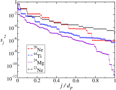
Figure 1: Singular values $s_{j}^{2}$ for ground-states of ²⁰Ne ($\ast$, $d_{\cal P}=66$), ²²Ne ($\times$, $d_{\cal P}=66$), ⁴⁴Ti ($+$, $d_{\cal P}=190$), and ²⁴Mg ($\bullet$, $d_{\cal P}=495$).

In this paper, we present an alternative technique that efficiently factorizes shell-model ground-states and determines the optimal factors for a given truncation. We make the ansatz

$$|\psi\rangle=\sum_{j=1}^{\Omega}|p_{j}\rangle|n_{j}\rangle.$$ (3)

Here, the unknown factors are the ${\cal P}$-states $|p_{j}\rangle$ and the ${\cal N}$-states $|n_{j}\rangle$. The truncation is controlled by the parameter $\Omega$ which counts the number of desired factors. Figure 1 suggests that $\Omega\ll\min{\left(d_{\cal P},d_{\cal N}\right)}$ yields accurate approximations to shell-model ground-states. This is also the result of our numerical computations below.

Let $\hat{H}$ be the nuclear many-body Hamiltonian. The unknown ${\cal P}$-states $|p_{j}\rangle$ and ${\cal N}$-states $|n_{j}\rangle$ in Eq. (3) are obtained from a variation of the energy $E=\langle\psi|\hat{H}|\psi\rangle/\langle\psi|\psi\rangle$, which yields ($j=1,\ldots,\Omega$)

$$\sum_{i=1}^{\Omega}\left(\langle n_{j}|\hat{H}|n_{i}\rangle-E\langle n_{j}|n_{i}\rangle\right)|p_{i}\rangle = 0,$$

$$\sum_{i=1}^{\Omega}\left(\langle p_{j}|\hat{H}|p_{i}\rangle-E\langle p_{j}|p_{i}\rangle\right)|n_{i}\rangle = 0.$$ (4)

These nonlinear equations are not easy to solve simultaneously. Note however that for fixed neutron (proton) states the first (second) set of these equations constitutes a generalized eigenvalue problem for the proton (neutron) states. Consider the first set of the Eqs. (Factorization of shell-model ground-states). The operator $\langle n_{i}|\hat{H}|n_{j}\rangle$ acts on ${\cal P}$-space and is determined by the nuclear structure Hamiltonian

$$\hat{H}=\hat{H}_{\cal N}+\hat{H}_{\cal P}+\hat{V}_{\cal PN},$$ (5)

with

$$\hat{H}_{\cal N} = \sum_{n}\varepsilon_{n}\hat{a}_{n}^{\dagger}\hat{a}_{n}+{1\over 4}\sum_{n,n^{\prime},m,m^{\prime}}v_{nn^{\prime}m^{\prime}m}\hat{a}_{n}^{\dagger}\hat{a}^{\dagger}_{n^{\prime}}\hat{a}_{m}\hat{a}_{m^{\prime}},$$

$$\hat{H}_{\cal P} = \sum_{p}\varepsilon_{p}\hat{a}_{p}^{\dagger}\hat{a}_{p}+{1\over 4}\sum_{p,p^{\prime},q,q^{\prime}}v_{pp^{\prime}q^{\prime}q}\hat{a}_{p}^{\dagger}\hat{a}^{\dagger}_{p^{\prime}}\hat{a}_{q}\hat{a}_{q^{\prime}},$$ (6)

$$\hat{V}_{\cal PN} = \sum_{p,n,n^{\prime},p^{\prime}}v_{pnp^{\prime}n^{\prime}}\hat{a}_{p}^{\dagger}\hat{a}^{\dagger}_{n}\hat{a}_{n^{\prime}}\hat{a}_{p^{\prime}}.$$

Here, we use indices $p,q$ and $m,n$ to refer to proton and neutron orbitals, respectively. The antisymmetric two-body matrix elements are denoted as $v_{ijkl}$.

Thus, the ${\cal P}$-space Hamilton operator $\langle n_{j}|\hat{H}|n_{i}\rangle$ is

$$\langle n_{i}|\hat{H}|n_{j}\rangle = \sum_{p,p^{\prime}}\left(\sum_{n,n^{\prime}}v_{pnp^{\prime}n^{\prime}}\langle n_{i}|\hat{a}^{\dagger}_{n}\hat{a}_{n^{\prime}}|n_{j}\rangle\right)\hat{a}_{p}^{\dagger}\hat{a}_{p^{\prime}}$$ (7)

$$+ \langle n_{i}|\hat{H}_{\cal N}|n_{j}\rangle+\langle n_{i}|n_{j}\rangle\hat{H}_{\cal P}.$$

Note that the neutron-proton interaction $\hat{V}_{\cal PN}$ results into a one-body proton operator while the neutron Hamiltonian $\hat{H}_{\cal N}$ yields a constant. This concludes the detailed explanation of the first set of equations in Eq. (Factorization of shell-model ground-states). The second set has an identical structure, only the role of neutrons and protons is reversed.

We solve the coupled set of nonlinear equations (Factorization of shell-model ground-states) iteratively as follows. We choose a random set of initial ${\cal N}$-states $\{|n_{j}\rangle,j=1,\ldots,\Omega\}$ and solve the first set of Eq. (Factorization of shell-model ground-states) for those ${\cal P}$-states $\{|p_{j}\rangle,j=1,\ldots,\Omega\}$ that yield the lowest energy $E$. We then use this solution for the second set of Eq. (Factorization of shell-model ground-states) which yields improved ${\cal N}$-states $\{|n_{j}\rangle,j=1,\ldots,\Omega\}$. We iterate this procedure until the energy $E$ is converged, typically 5-20 times. The advantage of the factorization method is that the dimensionality of the eigenvalue problem is $\Omega\times\max{(d_{\cal P},d_{\cal N})}$ while an exact diagonalization scales like $d_{\cal P}\times d_{\cal N}$. Before we present numerical results we note two further developments of the method. First, we will exploit the non-uniqueness of the ansatz (3) to reduce the generalized eigenvalue problem to a standard eigenvalue problem. Second, we will use the rotational symmetry of the shell-model Hamiltonian (5) to give a $m$-scheme formulation of the factorization method.

To reduce the Eqs. (Factorization of shell-model ground-states) to a standard eigenvalue problem we choose an orthonormal set of initial ${\cal N}$-states $\{|n_{j}\rangle,j=1,\ldots,\Omega\}$ as input to the first eigenvalue problem. This reduces the “overlap” matrix $\langle n_{j}|n_{i}\rangle$ to a unit matrix, and we solve a standard eigenvalue problem to obtain the ${\cal P}$-states $\{|p_{j}\rangle,j=1,\ldots,\Omega\}$. The resulting ${\cal P}$-states will not be orthogonal in general. Their coefficient matrix $C$ with elements $C_{\alpha j}\equiv\langle\pi_{\alpha}|p_{j}\rangle$ may, however, be factorized in a singular value decomposition as $C=UDV^{T}$. Here $D$ denotes a diagonal $\Omega\times\Omega$ matrix while $U$ is a (column) orthogonal $d_{\cal P}\times\Omega$ matrix, and $V$ is a orthogonal $\Omega\times\Omega$ matrix. The transformed states ($j=1,\ldots,\Omega$)

$$|p_{j}^{\prime}\rangle = \sum_{\alpha=1}^{d_{\cal P}}U_{\alpha,j}|\pi_{\alpha}\rangle,$$

$$|n_{j}^{\prime}\rangle = \sum_{i=1}^{\Omega}V_{ij}|n_{i}\rangle$$

are orthonormal in ${\cal P}$-space and ${\cal N}$-space, respectively, and fulfill

$$|\psi\rangle=\sum_{j=1}^{\Omega}|p_{j}\rangle|n_{j}\rangle=\sum_{j=1}^{\Omega}D_{jj}|p_{j}^{\prime}\rangle|n_{j}^{\prime}\rangle.$$ (8)

We then input the new ${\cal P}$-states $\{|p_{j}^{\prime}\rangle,j=1,\ldots,\Omega\}$ to the second set in Eq. (Factorization of shell-model ground-states), which poses a standard eigenvalue problem for the ${\cal N}$-states. The transformed neutron states $D_{jj}|n^{\prime}_{j}\rangle$ are good starting vectors for the Lanczos iteration. We iterate the whole procedure until the ground-state energy converges to an appropriate level of accuracy. Note that the singular value decomposition is very inexpensive compared to the diagonalization. This procedure also has the advantage that it yields the singular values $D_{jj}$ of the ground-state factorization.

	44Ti		48Cr		52Fe		56Ni
	$E_{0}$ [MeV]	$d$	$E_{0}$ [MeV]	$d$	$E_{0}$ [MeV]	$d$	$E_{0}$ [MeV]	$d$
Factorization	-10.74	190	-29.55	4,845	-50.41	38,760	-76.23	125,970
$m$-scheme Fact.	-12.74	190	-31.06	4,845	-52.03	38,760	-77.1	125,970
Exact	-13.88	4,000	-32.95	1,963,461	-54.27	109,954,620	-78.46	1, 087,455,228

Table 1:

Results for ground-state energies $E_{0}$ of $pf$-shell nuclei obtained from the factorization with just one state and the most severe $m$-scheme factorization compared to the exact results from Ref. Nathan . The $m$-scheme dimension of the corresponding eigenvalue problem, $d$, is also listed.

To include the axial symmetry (“$m$-scheme”) into the factorization we consider only products of proton and neutron states that have angular momentum projection $J_{z}=0$. To this purpose we modify the ansatz (3) as

$$|\psi\rangle=\sum_{m}\sum_{j=1}^{\Omega_{m}}|p_{j}^{(m)}\rangle|n_{j}^{(-m)}\rangle,$$ (9)

where $|p_{j}^{(m)}\rangle,j=1,\ldots,\Omega_{m}$ ($|n_{j}^{(-m)}\rangle,j=1,\ldots,\Omega_{m}$) denote many-proton states (many-neutron states) with angular momentum projection $J_{z}=m$ ($J_{z}=-m$), and the sum over $m$ runs over all value of $J_{z}$ that are realized. The ansatz (9) again leads to a generalized eigenvalue problem similar to Eq. (Factorization of shell-model ground-states), which we also cast into a standard eigenvalue problem by maintaining orthogonality between ${\cal P}$-states and between the ${\cal N}$-states through singular value decompositions. The number of factors used in the $m$-scheme factorization is given by the parameters $\Omega_{m}$. In the following, we use

$$\Omega_{m}(\alpha)=\max{\left(1,\alpha\Omega_{m}^{\rm max}\right)},$$ (10)

where $\Omega_{m}^{\rm max}$ is the maximal dimension of the corresponding subspace. For $\alpha=0$ the most severe truncation is obtained while $\alpha=1$ leads to an eigenvalue problem with the same dimension as an exact diagonalization in $m$-scheme. In the latter case, the first iteration (i.e. solving the first set of Eq. (Factorization of shell-model ground-states) for the proton states and using random, orthonormal neutron states as input) leads to the exact solution. This is due to the non-uniqueness of the ansatz (9). Note that other abelian symmetries and point symmetries can implemented in a similar manner as the axial symmetry. This flexibility is important since it allows us to consider factorizations that differ from the neutron-proton factorization proposed here. In neutron rich nuclei, for instance, there might be a large imbalance between the sizes of the proton and neutron space. In such a situation one might consider a “mixed” factorization where part of the neutron orbitals and all proton orbitals constitute one factor space while the other factor space consists of the remaining neutron orbitals. Note also that factorization method proposed here is not restricted to nuclear structure problems but could well be applied to problems in quantum chemistry or condensed matter.

We turn to numerical tests of the factorization method. We solve the eigenvalue equations with the sparse matrix solver arpack arpack . In a first step we set $\Omega=1$ in the ansatz (3) and compare the most severely truncated factorization with exact diagonalization. The factorization requires us to iteratively solve eigenvalue problems with rather low dimension $d_{\cal P}$ and $d_{\cal N}$, respectively. Table 1 shows the results for the $pf$-shell nuclei ⁴⁴Ti, ⁴⁸Cr, ⁵²Fe, and ⁵⁶Ni. The results from the severely truncated factorization deviate about 2-4 MeV from the exact results (from Ref. Nathan ). For comparison, we also list the dimension of the eigenvalue problem. It is also interesting to use the $m$-scheme factorization and set $\Omega_{m}=1$ in Eq. (9). This corresponds to $\alpha=0$ in Eq. (10) and yields a problem of equal dimension as the factorization (3) with truncation $\Omega=1$. Results are also listed in Table 1. The advantage of the $m$-scheme factorization is clearly visible as the corresponding results typically differ only 1-2 MeV from the exact results. This makes this severe truncation particularly interesting to compute good starting vectors for large-scale nuclear structure problems. After these encouraging results we will in the following include more factors to obtain more accurate ground-state factorizations.

We use the $m$-scheme factorization to compute accurate approximations to ground-state energies. As a first test case we consider the $sd$-shell nucleus ²⁴Mg with the USD interaction BW . The exact diagonalization yields the ground-states energy $E_{0}=-87.08$ MeV and has $m$-scheme dimension $d_{\rm max}=28503$. We solve the eigenvalue problem (Factorization of shell-model ground-states) for the ground state but also record a few excited energy solutions. The hollow data points in Fig. 2 show the resulting excitation spectrum versus the dimension of the eigenvalue problem relative to the dimension of the full $m$-scheme diagonalization, $d/d_{\rm max}$. The ground-state converges very fast while the excited states converge somewhat slower toward the exact results. To obtain fast converging results for the excited states, we directly solve the eigenvalue problem (Factorization of shell-model ground-states) for excited energies. The full data points in Fig. 2 show the results of such calculations for the first and second excited state, respectively.

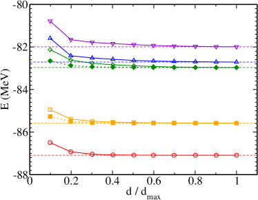
Figure 2: Low-energy spectrum for ²⁴Mg (USD interaction) versus the relative dimension of the eigenvalue problem. The dashed lines are the exact results, the open data points result from targeting the ground-state, and the filled data points result from directly targeting the 1^st and 2^nd excited state, respectively.

Figure 3 shows the squared overlaps of the factorization results with the exact solution versus the dimension $d$ of the eigenvalue problem. Excellent results are obtained for the ground state (which was directly targeted) and for the excited states. The inset of Fig. 3 shows that the angular momenta of the low-lying states are accurately reproduced even at severe truncations. This indicates that transition matrix elements can also be calculated very accurately. The results of Fig. 2 and Fig. 3 clearly demonstrate the efficiency and accuracy of the factorization.

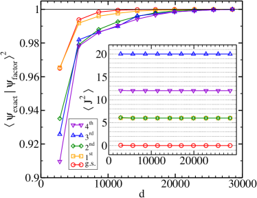
Figure 3: Squared wave function overlaps with the exact results for the low-lying states in ²⁴Mg (USD interaction) versus the dimension of the eigenvalue problem. Inset: Corresponding angular momentum expectation values. The results are obtained from targeting the ground state.

For $pf$-shell nuclei we use the KB3 interaction KB and compute the ground-states of ⁵⁶Ni and ⁴⁸Cr. The respective $m$-scheme dimensions are $d_{\rm max}=1.087\times 10^{9}$ and $d_{\rm max}=1.96\times 10^{6}$. Figure 4 shows the ground-state energies for ⁵⁶Ni and ⁴⁸Cr (inset) plotted versus the relative dimension $d/d_{\rm max}$ of the respective eigenvalue problem. We also show an exponential fit of the form $E(d/d_{\rm max})=E_{0}+b\exp{(-cd/d_{\rm max})}$ to the rightmost seven and six data points, respectively. For ⁵⁶Ni (⁴⁸Cr) the resulting ground-state energy is only 100 keV (30keV) above the exact result while the dimension of the eigenvalue problem is dramatically reduced by a factor 1000 (factor 12). Figure  5 shows the excitation spectrum relative to the ground-state. Our method reproduces the level spacings of the two lowest excitations very accurately even at the most severe truncation, while the spacings to the higher levels are about 300 keV too large. Quantum numbers are reproduced accurately for $d/d_{\rm max}\gtrsim 0.05$. Considering the modest size of the eigenvalue problem we solved, these are very good results. We also compared the $m$-scheme factorization with a particle-hole calculation. The results are listed in Table 2 and clearly demonstrate the fast convergence of the factorization method.

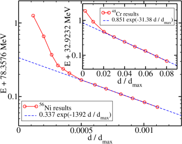
Figure 4: Ground-state energy $E$ versus the dimension $d$ of the eigenvalue problem relative to the $m$-scheme dimension $d_{\rm max}=1.087\times 10^{9}$ for ⁵⁶Ni. Inset: Similar plot for ⁴⁸Cr ($d_{\rm max}=1.96\times 10^{6}$).

Let us also compare the ground-state factorization presented in this work to three related methods. The DMRG also bases its truncation on the singular values White92 . Recent applications to simple nuclear structure problems were very successful Duk01 ; Duk02 , but the application to realistic nuclear structure problems seems more difficult as the convergence is very slow Dimitrova02 . Recently, Andreozzi and Porrini AP approximated the shell-model ground-state by products of eigenstates of the proton-proton and neutron-neutron Hamiltonian. This method yields quite good results for energy spacings of low-lying shell-model states. However, the generation of the eigenstates might become impractical for the large proton and neutron spaces. A third related method is the Exponential Convergence Method (ECM) Horoi94 ; Horoi99 ; Horoi02 ; Horoi03 . A direct comparison is not easy since the FPD6 interaction is used for $pf$-shell nuclei, and since ECM results are plotted versus $JT$-coupled dimension of the truncated space. However, it seems that the convergence of our method is considerably faster. For ⁴⁸Cr, for instance, our rate of exponential convergence is $c\approx-31.38$ (See Fig. 4), which is about a factor eight larger than what is reported for the ECM in Fig. 1 of Ref.Horoi02 . For ⁵⁶Ni, our exponential rate is about a factor 200 larger than the ECM rate HoroiPC , and our identification of the exponential region requires a $m$-scheme dimension $d\approx 10^{6}$ (See Fig. 4) while the ECM requires an $m$-scheme dimension of 4-5 million HoroiPC .

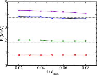
Figure 5: Level spacings of the lowest excitations with respect to the ground-state of the $pf$-shell nucleus ⁴⁸Cr (KB3 interaction) plotted versus the dimension $d$ of the eigenvalue problem relative to the $m$-scheme dimension $d_{\rm max}$. The dashed lines are the exact results.

In summary, we proposed a new method that factorizes ground-states of realistic nuclear structure Hamiltonians. The optimal factors are derived from a variational principle and are the solution of rather low-dimensional eigenvalue problems. The approximated states and energies converge exponentially quickly as more factors are included, and quantum numbers are accurately reproduced. Computations for $sd$-shell and $pf$-shell nuclei show that highly accurate approximations may result from eigenvalue problems whose dimensions are reduced by orders of magnitude.

$m$-scheme fact.		p-h approach
$E_{0}$ [MeV]	$d$		$E_{0}$ [MeV]	$d$
-31.06	4,845	2p-2h	-31.11	62,220
-32.68	78,407	4p-4h	-32.62	736,546
-32.83	138,386	5p-5h	-32.83	1,328,992

Table 2:

Comparison of $m$-scheme factorization method with a particle-hole calculation for ⁴⁸Cr (KB3 interaction). $d$ denotes the dimension of the corresponding eigenvalue problem.

The authors thank G. Stoitcheva for useful discussions and help in the uncoupling of matrix elements, and acknowledge communications with M. Horoi. This research used resources of the Center for Computational Sciences at Oak Ridge National Laboratory, and was supported in part by the U.S. Department of Energy under Contract Nos. DE-FG02-96ER40963 (University of Tennessee) and DE-AC05-00OR22725 with UT-Battelle, LLC (Oak Ridge National Laboratory).

References

- (1) E. Caurier, A. P. Zuker, A. Poves, and G. Martínez-Pinedo, Phys. Rev. C50, 225 (1994); [eprint nucl-th/9307001].
- (2) E. Caurier, G. Martínez-Pinedo, F. Nowacki, A. Poves, J. Retamosa, and A. P. Zuker, Phys. Rev. C59, 2033 (1999); [eprint nucl-th/9809068].
- (3) P. Navrátil, J. P. Vary, and B. R. Barrett, Phys. Rev. Lett. 84 (2000) 5728; [eprint nucl-th/0004058]; Phys. Rev. C62, 054311 (2000).
- (4) P. Navrátil and W. E. Ormand, Phys. Rev. Lett. 88, 152502 (2002).
- (5) S. C. Pieper and R. B. Wiringa, Ann. Rev. Nucl. Part. Sci. 51, 53 (2001); [eprint nucl-th/0103005].
- (6) S. C. Pieper, K. Varga, R. B. Wiringa, Phys. Rev. C66,044310 (2002); [eprint nucl-th/0206061].
- (7) G. H. Lang, C. W. Johnson, S. E. Koonin, and W. E. Ormand, Phys. Rev. C48, 1518 (1993); [eprint nucl-th/9305009].
- (8) S. E. Koonin, D. J. Dean, and K. Langanke, Phys. Rep. 278, 1 (1997); [eprint nucl-th/9602006].
- (9) M. Honma, T. Mizusaki, and T. Otsuka, Phys. Rev. Lett. 75, 1284 (1995).
- (10) M. Horoi, B. A. Brown, and V. Zelevinsky, Phys. Rev. C50, R2274 (1994); [eprint nucl-th/9406004].
- (11) M. Horoi, A. Voyla, and V. Zelevinsky, Phys. Rev. Lett. 82, 2064 (1999); [eprint nucl-th/9806015].
- (12) M. Horoi, B. A. Brown, and V. Zelevinsky, Phys. Rev. C65, 027303 (2002).
- (13) M. Horoi, B. A. Brown, and V. Zelevinsky, Phys. Rev. C67, 034303 (2003).
- (14) J. Dukelsky and S. Pittel, Phys. Rev. C63, 061303 (2001); [eprint nucl-th/0101048].
- (15) J. Dukelsky and S. Pittel, S. S. Dimitrova, and M. V. Stoitsov, Phys. Rev. C65, 054319 (2002); [eprint nucl-th/0202048].
- (16) S. S. Dimitrova, S. Pittel, J. Dukelsky, and M. V. Stoitsov, eprint nucl-th/0207025.
- (17) B. A. Brown and B. H. Wildenthal, Ann. Rev. Nucl. Part. Sci. 38, 29 (1988).
- (18) T. T. S. Kuo and G. E. Brown, Nucl. Phys. A 114, 241 (1968); A. Poves and A. P. Zuker, Phys. Rep. 70, 235 (1980).
- (19) S. R. White, Phys. Rev. Lett. 69, 2863 (1992); Phys. Rev. B48, 10345 (1993).
- (20) R. B. Lehoucq, D. C. Sorensen, and C. Yang, ARPACK User’s Guide (SIAM, Philadelphia 1998).
- (21) F. Andreozzi and A. Porrino, J. Phys. G 27, 845 (2001).
- (22) M. Horoi, private communication.