Nuclear Problems in Astrophysics

Abstract

These lectures, presented at the International School of Physics “Enrico Fermi,” deal with two major themes. The first is the remarkable story of the solar neutrino problem, which (along with the atmospheric neutrino anomaly) recently led to the discovery of massive neutrinos and neutrino oscillations, physics beyond the standard model. I will describe the physics of the standard solar model (SSM), the experimental program that was motivated by the discrepancies between SSM predictions and the initial observations of Raymond Davis, Jr., and his colleagues, and the recent results of SNO and SuperKamiokande. These first lectures end with a description of what we have learned about neutrino oscillations and the neutrino mass matrix, as well as the open questions (neutrino charge conjugation properties, the absolute mass scale, CP violation) that could ultimately impact our understanding of baryogenesis, the origin of large-scale structure, and other topics in cosmology and astrophysics. The second theme is the core-collapse supernova mechanism and associated nucleosynthesis. This problem connects neutrino physics, which controls much of the nuclear physics of the star, with the long-term chemical evolution of our galaxy. In particular, the $r$-process, which produces about half of the heavy elements, remains poorly understood, despite important new constraints from studies of metal-poor halo stars. The possible role of new neutrino properties on both the explosion mechanism and nucleosynthesis is noted.

1 Introduction

These lectures were presented at the International School of Physics “Enrico Fermi,” August 6-16, 2002, “From Nuclei and their Constituents to Stars.” This written version includes a few new results from later in 2002, such as the recent announcement by the KamLAND collaboration.

The main theme of these lectures is the interplay between neutrino properties — their mass, mixing, and behavior under charge conjugation and CP — and astrophysical phenomena. The first topic is the solar neutrino problem, in which the discrepancy between the predictions of the standard solar model (SSM) and the results of the chlorine experiment ultimately led to the discovery of neutrino oscillations by the SuperKamiokande and SNO collaborations. The lectures include a discussion of the basic physics of the SSM, the experiments on solar and atmospheric neutrinos, the effects of matter on neutrino oscillations, and the current status of our efforts to determine the neutrino mass matrix.

The second topic is one reminiscent of the solar neutrino problem in the 1970s, the core-collapse supernova mechanism. The failure thusfar to develop a robust theory of supernova explosions may indicate some basic inadequacy in our treatment of the nuclear astrophysics (such as our inability to model the hydrodynamics and transport realistically in three dimensions). But surprises could arise from new neutrino physics, as the environment (intense neutrino fluxes, high-velocity matter flow) is significantly different from any other we have probed. The supernova mechanism is important to basic astrophysics, as it controls much of the long-term chemical evolution of our galaxy: supernovae both synthesize and eject new elements. Futhermore, as a source of measureable fluxes of neutrinos of all flavors, supernovae offer experimentalists new opportunities to test neutrino properties. The lectures deal with supernova neutrino physics and with the nucleosynthesis associated directly (the $\nu$-process) and indirectly (the $r$-process) with neutrinos.

The “live” audience for these lectures was advanced graduate students and postdocs in nuclear and particle physics: the material is covered at this level and at a depth appropriate to a survey.

2 Solar Neutrinos [1]

The neutrino has been with us since Wolfgang Pauli’s proposal, in December, 1930, that the emission of an unobserved spin-1/2 neutral particle might explain the apparent lack of energy conservation in nuclear beta decay

$$(A,Z)\rightarrow(A,Z-1)+e^{+}+\nu.$$ (1)

Enrico Fermi was present at a number of Pauli’s presentations and discussed the neutrino with him on these occasions. In 1934, following closely Chadwick’s discovery of the neutron, Fermi proposed a theory of beta decay based on Dirac’s description of electromagnetic interactions, but with weak currents interacting at a point, rather than at long distance through the electromagnetic field. Beta decay was descibed as a proton decaying to a neutron, a phenomenon energetically possible because of nuclear binding energies, with the emission of a positron and neutrino. Apart from the absence of parity violation, which awaited discovery until 1957, Fermi’s description is a correct low-energy approximation to our current standard model of weak interactions.

The neutrino was connected early on to astrophysics. As Bethe, Critchfield, and others unraveled the stellar processes for hydrogen burning (the pp chain and CNO cycles), stars were recognized to be copious sources of neutrinos

$$4\mathrm{p}\rightarrow{}^{4}\mathrm{He}+2e^{+}+2\nu_{e}.$$ (2)

The detectability of neutrinos – of which Pauli had apologetically dispaired – was established by Cowan and Reines in 1956, and the existence of more than one flavor of neutrino by Lederman, Schwarz, and Steinberger in 1962. Thus, with the development of the Glashow-Weinberg-Salam electroweak standard model and its prediction of weak neutral currents, it was recognized that supernovae would emit prodigous numbers of neutrinos of all flavors: the hot protoneutron star at the core of the collapse contains a thermal sea of trapped neutrinos produced via neutal currents. Questions of astrophysics and of neutrino properties are thus interwined, and much can be learned about one by improving our understanding of the other.

More than three decades ago Ray Davis, Jr. and his collaborators [2] constructed a 0.615 kiloton C₂Cl₄ radiochemical solar neutrino detector in the Homestake Gold Mine, one mile beneath Lead, South Dakota. This experiment began a field, neutrino astrophysics, that in the past few years has produced remarkable discoveries showing that our current standard electroweak model is incomplete. The new neutrino properties that have been established – neutrinos are massive and neutrino flavors strongly mix – provide our first glimpse of new interactions that likely reside at energies far beyond the limits of current accelerators. Furthermore, the discoveries have important implications for particle dark matter, large-scale structure, and models where the baryon number asymmetry is connected to leptogenesis.

The first few years of the Davis experiment showed that the number of neutrinos detected was considerably below the predictions of the SSM, that is, the standard theory of main sequence stellar evolution. Those results were refined over the 30-year lifetime of the experiment, which ultimately achieved a precision equivalent to about 3% of the SSM prediction. The Cl experiment was followed by the SAGE [3] and GALLEX/GNO [4, 5] gallium experiments, the Kamiokande [6] and SuperKamiokande [7] water Cerenkov detectors, and the SNO heavy water Cerenkov detector [8]. Furthermore the explanation for the discrepancy that was inexorably forced on us – massive neutrinos oscillating as they travel from the sun’s core to the earth – proved to account for a similar anomaly in atmospheric neutrino measurements [9]. These new neutrino properties are now being confirmed with accelerator and reactor neutrino experiments, such as K2K and KamLAND. Ultimately a series of long- and short-baseline accelerator/reactor experiments coupled with new astrophysical measurements will yield precise values for the mixing parameters and probe new phenoma, such as CP violation.

My goal in the first half of these lectures is to summarize the solar neutrino problem – the standard solar model, the observations, and the accumulated evidence that led to neutrino oscillations as a resolution. The status of our knowledge of the neutrino mass matrix will be given, as well as the exciting set of outstanding questions – particle-antiparticle conjugation properties, CP violation, absolute scale of neutrino mass, the mass hierarchy, implications for dark matter and large-scale structure, connections with baryogenesis – remaining to be resolved. This is one of those wonderful times in physics where not only are new discoveries in hand, but we know we have the capacity experimentally to seek solutions to even deeper questions.

2.1 The Standard Solar Model [10]

Observations of stars reveal a wide variety of stellar conditions, with luminosities relative to solar spanning a range $L\sim 10^{-4}$ to $10^{6}L_{\odot}$ and surface temperatures $T_{s}\sim 2000-50000$K. The simplest relation one could propose between luminosity and $T_{s}$ is that for a blackbody

$$L=4\pi R^{2}\sigma T_{s}^{4}\Rightarrow$$

$${L\over L_{\odot}}=({R\over R_{\odot}})^{2}({T_{s}\over T_{\odot}})^{4},$$ (3)

which suggests that stars of a similar structure might lie along a one-parameter path (corresponding to $R/R_{\odot}$ above) in the luminosity (or magnitude) vs. temperature (or color) plane. In fact, there is a dominant path in the Hertzsprung-Russell color-magnitude diagram along which roughly 80% of the stars lie. This is the main sequence, those stars supporting themselves by hydrogen burning through the pp chain or CNO cycles.

As one such star, the sun is an important test of our theory of main sequence stellar evolution: its properties – age, mass, surface composition, luminosity, and helioseismology – are by far the most accurately known among the stars. The SSM traces the evolution of the Sun over the past 4.6 billion years of main sequence burning, thereby predicting the present-day temperature and composition profiles of the solar core that govern neutrino production. Standard solar models share four basic assumptions:

$\bullet$ The sun evolves in hydrostatic equilibrium, maintaining a local balance between the gravitational force and the pressure gradient. To describe this condition in detail, one must specify the equation of state as a function of temperature, density, and composition.

$\bullet$ Energy is transported by radiation and convection. While the solar envelope is convective, radiative transport dominates in the core region where thermonuclear reactions take place. The opacity depends sensitively on the solar composition, particularly the abundances of heavier elements.

$\bullet$ Thermonuclear reaction chains generate solar energy. The standard model predicts that over 98% of this energy is produced from the pp chain conversion of four protons into ⁴He (see fig. 1), with proton burning through the CNO cycle contributing the remaining 2%. The Sun is a large but slow reactor: the core temperature, $T_{c}\sim 1.5\cdot 10^{7}$ K, results in typical center-of-mass energies for reacting particles of $\sim$ 10 keV, much less than the Coulomb barriers inhibiting charged particle nuclear reactions. Thus reaction cross sections are small: in most cases, as laboratory measurements are only possible at higher energies, cross section data must be extrapolated to the solar energies of interest.

$\bullet$ The model is constrained to produce today’s solar radius, mass, and luminosity. An important assumption of the standard model is that the Sun was highly convective, and therefore uniform in composition, when it first entered the main sequence. It is furthermore assumed that the surface abundances of metals (nuclei with A $>$ 5) were undisturbed by the subsequent evolution, and thus provide a record of the initial solar metallicity. The remaining parameter is the initial ⁴He/H ratio, which is adjusted until the model reproduces the present solar luminosity after 4.6 billion years of evolution. The resulting ⁴He/H mass fraction ratio is typically 0.27 $\pm$ 0.01, which can be compared to the big-bang value of 0.23 $\pm$ 0.01. Note that the Sun was formed from previously processed material.

Figure 1: The solar pp chain.

The model that emerges is an evolving Sun. As the core’s chemical composition changes, the opacity and core temperature rise, producing a 44% luminosity increase since the onset of the main sequence. The temperature rise governs the competition between the three cycles of the pp chain: the ppI cycle dominates below about 1.6 $\cdot 10^{7}$ K; the ppII cycle between (1.7-2.3) $\cdot 10^{7}$K; and the ppIII above 2.4 $\cdot 10^{7}$K. The central core temperature of today’s SSM is about 1.55 $\cdot 10^{7}$K.

The competition between the cycles determines the pattern of neutrino fluxes. Thus one consequence of the thermal evolution of our sun is that the ⁸B neutrino flux, the most temperature-dependent component, proves to be of relatively recent origin: the predicted flux increases exponentially with a doubling period of about 0.9 billion years.

A final aspect of SSM evolution is the formation of composition gradients on nuclear burning timescales. Clearly there is a gradual enrichment of the solar core in ⁴He, the ashes of the pp chain. Another element, ³He, is produced and then consumed in the pp chain, eventually reaching some equilibrium abundance. The timescale for equilibrium to be established as well as the eventual equilibrium abundance are both sharply decreasing functions of temperature, and thus increasing functions of the distance from the center of the core. Thus a steep ³He density gradient is established over time.

The SSM has had some notable successes. From helioseismology the sound speed profile $c(r)$ has been very accurately determined for the outer 90% of the Sun, and is in excellent agreement with the SSM. Such studies verify important predictions of the SSM, such as the depth of the convective zone. However the SSM is not a complete model in that it does not explain all features of solar structure, such as the depletion of surface Li by two orders of magnitude. This is usually attributed to convective processes that operated at some epoch in our sun’s history, dredging Li to a depth where burning takes place.

The principal neutrino-producing reactions of the pp chain and CNO cycle are summarized in Table 1. The first six reactions produce $\beta$ decay neutrino spectra having allowed shapes with endpoints given by E${}_{\nu}^{\rm max}$. Deviations from an allowed spectrum occur for ⁸B neutrinos because the ⁸Be final state is a broad resonance. The last two reactions produce line sources of electron capture neutrinos, with widths $\sim$ 2 keV characteristic of the temperature of the solar core. Measurements of the pp, ⁷Be, and ⁸B neutrino fluxes will determine the relative contributions of the ppI, ppII, and ppIII cycles to solar energy generation. As discussed above, and as later illustrations will show more clearly, the competition between these cycles is governed in large classes of solar models by a single parameter, the central temperature $T_{c}$. The flux predictions of the 1998 calculations of Bahcall, Basu, and Pinsonneault [10] (BP98) and of Brun, Turck-Chieze and Morel [11] are included in Table 1.

Table 1: Solar neutrino sources and the flux predictions of the Bahcall/Pinsonneault (BP98) and Brun/Turck-Chieze/Morel (BTCM98) SSMs in cm^-2s^-1.

Source	E${}_{\nu}^{max}$ (MeV)	BP98	BTCM98
p + p $\rightarrow^{2}$H + e${}^{+}+\nu$	0.42	5.94E10	5.98E10
13N $\rightarrow^{13}$C + e${}^{+}+\nu$	1.20	6.05E8	4.66E8
15O $\rightarrow^{15}$N + e${}^{+}+\nu$	1.73	5.32E8	3.97E8
17F $\rightarrow^{17}$O + e${}^{+}+\nu$	1.74	6.33E6
8B $\rightarrow^{8}$Be + e${}^{+}+\nu$	$\sim$ 15	5.15E6	4.82E6
3He + p $\rightarrow^{4}$He + e${}^{+}+\nu$	18.77	2.10E3
7Be + e${}^{-}\rightarrow^{7}$Li + $\nu$	0.86 (90%)	4.80E9	4.70E9
	0.38 (10%)
p + e- + p $\rightarrow^{2}$H + $\nu$	1.44	1.39E8	1.41E8

2.2 Solar Neutrino Detection [12]

Let us start with a brief reminder about low energy neutrino-nucleus interactions in detectors. Consider the charged current reaction

$$\nu_{e}+(A,Z)\rightarrow e^{-}+(A,Z+1)$$ (4)

Because the momentum transfer to the nucleus is very small for solar neutrinos, it can be neglected in the weak propagator, leading to an effective contact current-current interaction. If we begin with the simplest example of a semileptonic weak process, the decay of a free neutron n $rightarrow$ p$+e^{-}+\bar{\nu}_{e}$, the corresponding transition amplitude is then

$$S_{fi}={G_{F}\over\sqrt{2}}\cos\theta_{C}\bar{u}(\mathrm{p})\gamma_{\mu}(1-g_{A}\gamma_{5})u(\mathrm{n})\bar{u}(e)\gamma^{\mu}(1-\gamma_{5})u(\nu)$$ (5)

where $G_{F}$ is the weak coupling constant measured in muon decay and $\cos\theta_{c}$ gives the amplitude for the weak interaction to connect the u quark to its first-generation partner, the d quark. The origin of this effective amplitude is the underlying standard model predictions for the elementary quark and lepton currents, which are exactly left handed. Experiment shows that the effective coupling of the W boson to the nucleon is governed by $\gamma_{\mu}(1-g_{A}\gamma_{5})$, as noted above, where $g_{A}\sim 1.26$. The axial coupling is thus shifted from its underlying value by the strong interactions responsible for the binding of the quarks within the nucleon.

If an isolated nucleon were the target, one could proceed to calculate the cross section from the effective nucleon current given above. The extension to nuclear systems traditionally begins with the observation that nucleons in the nucleus are rather non-relativistic, $v/c\sim 0.1$. The amplitude $\bar{u}$(p)$\gamma^{\mu}(1-g_{A}\gamma_{5})u$(n) can be expanded in powers of $p/M$. The leading vector and axial operators are readily found to be

$$\gamma_{0} : ~{}~{}~{}1$$

$$\vec{\gamma} : ~{}~{}~{}\vec{p}/M\sim v/c$$

$$\gamma_{0}\gamma_{5} : ~{}~{}~{}\vec{\sigma}\cdot\vec{p}/M\sim v/c$$

$$\vec{\gamma}\gamma_{5} : ~{}~{}~{}\vec{\sigma}$$ (6)

Thus it is the time-like part of the vector current and the space-like part of the axial-vector current that survive in the non-relativistic limit.

If such a non-relativistic reduction is done for our single-nucleon current one obtains

$$S_{fi} \sim \cos\theta_{c}{G_{F}\over\sqrt{2}}(\phi^{\dagger}(\mathrm{p})\phi(\mathrm{n})\bar{u}(e)\gamma^{0}(1-\gamma_{5})u(\nu)$$ (7)

$$-\phi^{\dagger}(\mathrm{p})g_{A}\vec{\sigma}\phi(\mathrm{n})\cdot\bar{u}(e)\vec{\gamma}(1-\gamma_{5})u(\nu))$$

where the $\phi$’s are now two-component Pauli spinors for the nucleons. The above result can be extended to include $\bar{\nu}_{e}$ reactions by introducing the isospin operators $\tau_{\pm}$ where $\tau_{+}$ $\mid$ n$\rangle$ = $\mid$ p$\rangle$ and $\tau_{-}$$\mid$ p$\rangle$ = $\mid$ n$\rangle$, with all other matrix elements being zero. Thus we can generalize our n$\rightarrow$p amplitude to n$\leftrightarrow$p by

$$\phi^{\dagger}(\mathrm{p})\phi(\mathrm{n})\rightarrow\phi^{\dagger}(\mathrm{N})\tau_{\pm}\phi(\mathrm{N})$$

$$\phi^{\dagger}(\mathrm{p})\vec{\sigma}\phi(\mathrm{n})\rightarrow\phi^{\dagger}(\mathrm{N})\vec{\sigma}\tau_{\pm}\phi(\mathrm{N}).$$

This result easily generalizes to nuclear decay. Given our comments about exchange currents, the first step is the replacement

$$\tau_{\pm}\rightarrow\sum_{i=1}^{A}\tau_{\pm}(i)$$

$$\sigma\tau_{\pm}\rightarrow\sum_{i=1}^{A}\sigma(i)\tau_{\pm}(i).$$

Plugging $S_{fi}$ into the standard cross section formula (which involves an average over initial and sum over final nuclear spins of the square of the transition amplitude) then yields the allowed squared nuclear matrix element

$${1\over 2J_{i}+1}\left(|\langle f||\sum_{i=1}^{A}\tau_{\pm}(i)||i\rangle|^{2}+g_{A}^{2}|\langle f||\sum_{i=1}^{A}\sigma(i)\tau_{\pm}(i)||i\rangle|^{2}\right).$$ (8)

The Fermi operator is proportional to the isospin raising/lowering operator: in the limit of good isospin, which typically is broken at the $\mathrel{\hbox to0.0pt{\lower 4.0pt\hbox{\hskip 1.0pt$\sim$}\hss}\raise 1.0pt\hbox{$<$}}$ 5% level for transitions between well-bound nuclear states, the Fermi operator only connects states in the same isospin multiplet, that is, states with a common spin-spatial structure. If the initial state has isospin $(T_{i},M_{Ti})$, this final state has $(T_{i},M_{Ti}\pm 1)$ for $(\nu,e^{-})$ and $(\bar{\nu},e^{+})$ reactions, respectively, and is called the isospin analog state (IAS). In the limit of good isospin the sum rule for this operator in then particularly simple

$${1\over 2J_{i}+1}\sum_{f}|\langle f||\sum_{i=1}^{A}\tau_{+}(i)||i\rangle|^{2}={1\over 2J_{i}+1}|\langle IAS||\sum_{i=1}^{A}\tau_{+}(i)||i\rangle|^{2}=|N-Z|.$$ (9)

The excitation energy of the IAS relative to the parent ground state can be estimated accurately from the Coulomb energy difference

$$E_{IAS}\sim\left({1.728Z\over 1.12A^{1/3}+0.78}-1.293\right)\mathrm{MeV}.$$ (10)

The angular distribution of the outgoing electron for a pure Fermi $(N,Z)+\nu\rightarrow(N-1,Z+1)+e^{-}$ transition is 1 + $\beta\cos\theta_{e}$, and thus forward peaked. Here $\beta$ is the electron velocity.

The Gamow-Teller (GT) response is more complicated, as the operator connects the ground state to many states in the final nucleus. In general we do not have a precise probe of the nuclear GT response apart from weak interactions themselves. However a good approximate probe is provided by forward-angle (p,n) scattering off nuclei. The (p,n) studies demonstrate that the GT strength tends to concentrate in a broad resonance centered at a position $\delta=E_{GT}-E_{IAS}$ relative to the IAS given by

$$\delta\sim\left(7.0-28.9{N-Z\over A}\right)~{}\mathrm{MeV}.$$ (11)

Thus while the peak of the GT resonance is substantially above the IAS for $N\sim Z$ nuclei, it drops with increasing neutron excess, with $\delta\sim 0$ for Pb. A typical value for the full width at half maximum $\Gamma$ is $\sim$ 5 MeV. The angular distribution of GT $(N,Z)+\nu_{e}\rightarrow(N-1,Z+1)+e^{-}$ reactions is $3-\beta\cos\theta_{e}$, corresponding to a gentle peaking in the backward direction.

The above discussion of allowed responses can be repeated for neutral current processes such as $(\nu,\nu^{\prime})$. The analog of the Fermi operator contributes only to elastic processes, where the standard model nuclear weak charge is approximately the neutron number. As this operator does not generate transitions, it is not yet of much interest for solar or supernova neutrino detection, though there are efforts to develop low-threshold detectors (e.g., cryogenic technologies) for recording the modest nuclear recoil energies. The analog of the GT response involves

$$|M_{GT}^{fi}(\nu,\nu^{\prime})|^{2}={1\over 2J_{i}+1}|\langle f||\sum_{i=1}^{A}\sigma(i){\tau_{3}(i)\over 2}||i\rangle|^{2}.$$ (12)

The operator appearing in this expression is familiar from magnetic moments and magnetic transitions, where the large isovector magnetic moment ($\mu_{v}\sim$ 4.706) often leads to it dominating the orbital and isoscalar spin operators.

Finally, there is one purely leptonic reaction of great interest, since it is the reaction exploited by Kamiokande and SuperKamiokande. Electron neutrinos can scatter off electrons via both charged and neutral current reactions. The cross section calculation is straightforward and will not be repeated here. Two features of the result are of importance for our later discussions, however. Because of the neutral current contribution, heavy-flavor $(\nu_{\mu}$ and $\nu_{\tau})$ also scatter off electrons, but with a cross section reduced by about a factor of seven at low energies. Second, for neutrino energies well above the electron rest mass, the scattering is sharply forward peaked. Thus this reaction allows one to exploit the position of the Sun in separating the solar neutrino signal from a large but isotropic background.

As we mentioned earlier, the first experiment performed exploited the reaction

$${}^{37}\mathrm{Cl}(\nu,e^{-})^{37}\mathrm{Ar}.$$

As the threshold for this reaction is 0.814 MeV, the important neutrino sources are the ⁷Be and ⁸B fluxes. The ⁷Be neutrinos excite just the GT transition to the ground state, the strength of which is known from the electron capture lifetime of ³⁷Ar. The ⁸B neutrinos can excite all bound states in ³⁷Ar, including the dominant transition to the IAS residing at an excitation of 4.99 MeV. The strength of excite-state GT transitions can be determined from the $\beta$ decay ³⁷Ca$(\beta^{+})^{37}$K, which is the isospin mirror reaction to ³⁷Cl$(\nu,e^{-})^{37}$Ar. The net result is that, for SSM fluxes, 78% of the capture rate should be due to ⁸B neutrinos, and 15% to ⁷Be neutrinos. The measured capture rate [13] 2.56 $\pm 0.16\pm 0.16$ SNU (1 SNU = 10^-36 capture/atom/sec) is about 1/3 the standard model value.

Similar radiochemical experiments were done by the SAGE, GALLEX, and GNO collaborations using a different target, ⁷¹Ga. The special properties of this target include its low threshold and an unusually strong transition to the ground state of ⁷¹Ge, leading to a large pp neutrino cross section (see fig. 2). The experimental capture rates are $66^{+5.3+3.7}_{-5.2-3.2}$ and $74.1^{+5.4+4.0}_{-5.4-4.2}$ SNU for the SAGE (data through December, 2001) and GALLEX/GNO (data through GNOI) detectors, respectively. The SSM prediction is about 130 SNU [14]. Most important, since the pp flux is directly constrained by the solar luminosity in all steady-state models, there is a minimum theoretical value for the capture rate of 79 SNU, given standard model weak interaction physics. Uncertainties in the ⁷¹Ga cross section due to ⁷Be neutrino capture to two excited states of unknown strength were greatly reduced by direct calibrations of both detectors using ⁵¹Cr neutrino sources.

Figure 2: Level scheme for ⁷¹Ge showing the excited states that contribute to absorption of pp, ⁷Be, ⁵¹Cr, and ⁸B neutrinos.

The water Cerenkov experiments Kamiokande II/III and SuperKamiokande viewed solar neutrinos on an event-by-event basis. Solar neutrinos scatter off electrons, with the recoiling electrons producing the Cerenkov radiation that is then recorded in surrounding photo-tubes. Thresholds are determined by background rates; SuperKamiokande operated with triggers as low as 5 MeV. The initial experiment, Kamiokande II/III, found a flux of ⁸B neutrinos of (2.80 $\pm 0.19\pm 0.33)\cdot 10^{6}$/cm²s after about a decade of measurement. Its much larger successor SuperKamiokande, with a 22.5 kiloton fiducial volume, yielded the result $(2.35\pm 0.02\pm 0.08)\cdot 10^{6}$/cm²s after 1496 days of measurements [15], corresponding to 0.465 of the SSM ⁸B neutrino flux.

Results from the Sudbury Neutrino Observatory (SNO) will be discussed later in the lectures.

2.3 The Argument for New Particle Physics

The pattern of solar neutrino fluxes that has emerged from these experiments is

$$\phi(\mathrm{pp}) \sim 0.9\,\phi^{\rm{SSM}}(\mathrm{pp})$$

$$\phi(^{7}{\rm{Be}}) \sim 0$$

$$\phi(^{8}{\rm B}) \sim 0.43\,\phi^{\rm{SSM}}(^{8}{\rm B}).$$ (13)

A reduced ⁸B neutrino flux can be produced by lowering the central temperature of the sun somewhat, as $\phi(^{8}$B)$\sim T_{c}^{18}$. However, such an adjustment, either by varying the parameters of the SSM or by adopting some nonstandard physics, tends to push the $\phi(^{7}$Be)/$\phi(^{8}$B) ratio to higher values rather than the low one of eq. (13),

$${\phi(^{7}{\rm{Be}})\over\phi(^{8}{\rm B})}\sim T_{c}^{-10}.$$ (14)

Thus the observations seem difficult to reconcile with plausible solar model variations: one observable, $\phi(^{8}$B), requires a cooler core while a second, the ratio $\phi(^{7}$Be)/$\phi(^{8}$B), requires a hotter one.

How robust is this apparent contradiction? In the last decade, as evidence mounted that the solar neutrino problem was a profound one, a key issue was SSM uncertainties. Inputs into the SSM – pp chain nuclear cross sections, solar parameters like the age, luminosity, and composition, and atomic physics quantities such as opacities and screening corrections – all have measurement and theory errors. It was the care with which these uncertainties were assessed that convinced the community that the solar neutrino problem was a serious one.

No issue received more scrutiny that the nuclear cross sections. The pp chain involves a series of non-resonant charged-particle reactions occurring at center-of-mass energies that are well below the height of the inhibiting Coulomb barriers. As the resulting small cross sections generally preclude laboratory measurements at the relevant energies, one must extrapolate higher energy measurements to threshold to obtain solar cross sections. This extrapolation is usually discussed in terms of the astrophysical S-factor

$$\sigma(E)={S(E)\over E}\exp(-2\pi\eta)$$ (15)

where $\eta={Z_{1}Z_{2}\alpha\over\beta}$, with $\alpha$ the fine structure constant and $\beta=v/c$ the relative velocity of the colliding particles. This parameterization removes the gross Coulomb effects associated with the s-wave interactions of charged, point-like particles. The remaining energy dependence of S(E) is gentle and can be expressed as a low-order polynomial in E. Usually the variation of S(E) with E is taken from a direct reaction model and then used to extrapolate higher energy measurements to threshold. The model accounts for finite nuclear size effects, strong interaction effects, contributions from other partial waves, etc. As laboratory measurements are made with atomic nuclei while conditions in the solar core guarantee the complete ionization of light nuclei, additional corrections must be made to account for the different electronic screening environments.

Thus a great deal of effort was invested in laboratory measurements, in the theory required to extrapolate those measurements to the Gamow peak energies where solar reactions take place, and in assessing the resulting cross section uncertainties. In addition, other SSM uncertainties were evaluated. One qualitative illustration of the results is given by fig. 3, which summarizes a Monte Carlo study of SSM input parameter uncertainties. Five key input parameters, the primordial heavy-element-to-hydrogen ratio Z/X and S(0) for the p-p, ³He-³He, ³He-⁴He, and p-⁷Be were varied according to their assigned uncertainties, assuming for each parameter a normal distribution with the appropriate mean and standard deviation. (These five were the parameters assigned the largest uncertainties.) Smaller uncertainties from radiative opacities, the solar luminosity, and the solar age were folded into the results of the model calculations perturbatively [16, 17].

The resulting pattern of ⁷Be and ⁸B flux predictions produces an elongated error ellipse, showing that $\nu$ flux changes are strongly correlated even when a large set of distinct uncertainties are explored. Those variations producing $\phi(^{8}$B) below 0.8$\phi^{\rm{SSM}}(^{8}$B) tend to produce a reduced $\phi(^{7}$Be), but the reduction is always less than 0.8. Thus a greatly reduced $\phi(^{7}$Be) cannot be achieved within the uncertainties assigned to parameters in the SSM.

Figure 3: SSM ⁷Be and ${}^{8}B$ flux predictions. The dots represent the results of SSM calculations where the input parameters were varied according to their assigned uncertainties, as described in the text. The 90% and 99% confidence level error ellipses are shown.

A similar exploration, but including parameter variations very far from their preferred values, was carried out by Castellani et al. [18], who displayed their results as a function of the resulting core temperature $T_{c}$. The pattern that emerges is striking (see fig. 4): parameter variations producing the same value of $T_{c}$ produce remarkably similar fluxes. Thus $T_{c}$ provides an excellent one-parameter description of standard model perturbations. Figure 4 also illustrates the difficulty of producing a low ratio of $\phi(^{7}$Be)/$\phi(^{8}$B) when $T_{c}$ is reduced.

The Monte Carlo parameter variations of fig. 3 were constrained to reproduce the solar luminosity. Those variations show a similar strong correlation with $T_{c}$

$$\phi(\mathrm{pp})\propto T_{c}^{-1.2}~{}~{}~{}~{}~{}~{}~{}\phi(^{7}{\rm{Be}})\propto T_{c}^{8}~{}~{}~{}~{}~{}~{}~{}\phi(^{8}{\rm B})\propto T_{c}^{18}.$$ (16)

Figures 3 and 4 offer a strong argument that reasonable variations in the parameters of the SSM, or nonstandard changes in quantities like the metallicity, opacities, or solar age, cannot produce the pattern of fluxes deduced from experiment (eq. (13)). This would seem to limit possible solutions to errors either in the underlying physics of the SSM or in our understanding of neutrino properties.

Figure 4: The responses of the pp, ⁷Be, and ⁸B neutrino fluxes to the indicated variations in solar model input parameters, displayed as a function of the resulting central temperature $T_{c}$. From Castellani et al.

The Castellani et al. explorations belong to a larger class of proposed nonstandard solar models where either very large parameter changes (in nuclear cross sections, opacities, etc.) or new physics (e.g., mixing in the solar core) are hypothesized. Once results from Cl, SAGE/GALLEX, and Kamiokande were available, it became possible to argue that no such nonstandard solar model can solve the solar neutrino problem: if one assumes undistorted neutrino spectra, no combination of pp, ⁷Be, and ⁸B neutrino fluxes fits the experimental results well [19]. In fact, in an unconstrained fit, the required ⁷Be flux is unphysical, negative by almost 3$\sigma$. Thus, barring some unfortunate experimental error, new particle physics seemed to be the indicated solution. This conclusion was reinforced by the successes the SSM had in reproducing the new data on helioseismology [20]. Suggested particle physics solutions include neutrino oscillations, neutrino decay, neutrino magnetic moments, and weakly interacting massive particles. Among these, the Mikheyev-Smirnov-Wolfenstein effect — neutrino oscillations enhanced by matter interactions — was widely regarded as the most plausible.

2.4 Neutrino Oscillations

One odd feature of particle physics is that neutrinos, which are not required by any symmetry to be massless, nevertheless must be much lighter than any of the other known fermions. For instance, the current limit on the $\overline{\nu}_{e}$ mass is $\mathrel{\hbox to0.0pt{\lower 4.0pt\hbox{\hskip 1.0pt$\sim$}\hss}\raise 1.0pt\hbox{$<$}}$ 2.2 eV. The standard model requires neutrinos to be massless, but the reasons are not fundamental. Dirac mass terms $m_{D}$, analogous to the mass terms for other fermions, cannot be constructed because the model contains no right-handed neutrino fields. Neutrinos can also have Majorana mass terms

$$\overline{\nu^{c}_{L}}m_{L}\nu_{L}~{}~{}~{}\mathrm{and}~{}~{}\overline{\nu^{c}_{R}}m_{R}\nu_{R}$$ (17)

where the subscripts $L$ and $R$ denote left- and right-handed projections of the neutrino field $\nu$, and the superscript $c$ denotes charge conjugation. The first term above is constructed from left-handed fields, but can only arise as a nonrenormalizable effective interaction when one is constrained to generate $m_{L}$ with the doublet scalar field of the standard model. The second term is absent from the standard model because there are no right-handed neutrino fields.

None of these standard model arguments carries over to the more general, unified theories that theorists believe will supplant the standard model. In the enlarged multiplets of extended models it is natural to characterize the fermions of a single family, e.g., $\nu_{e}$, e, u, d, by the same (Dirac) mass scale $m_{D}$. Indeed the charged members of this multiplet all have comparable masses $\sim$ 1 MeV. The neutrino, however, is much lighter; but the neutrino, which carries no charge, is the only standard model fermion that can have both Majorana and Dirac mass terms. Thus it is natural to explain small neutrino masses as a consequence of Majorana masses. In the seesaw mechanism[21],

$$M_{\nu}\sim\left(\begin{array}[]{cc}0&m_{D}\\ m^{T}_{D}&m_{R}\end{array}\right).$$ (18)

Diagonalization of the mass matrix produces one light neutrino, $m_{\mathrm{light}}\sim{m_{D}^{2}\over m_{R}}$, and one unobservably heavy, $m_{\mathrm{heavy}}\sim m_{R}$. The factor ($m_{D}$/$m_{R}$) is the needed small parameter that accounts for the distinct scale of neutrino masses. The masses for the $\nu_{e},\nu_{\mu}$, and $\nu_{\tau}$ are then related to the squares of the corresponding quark masses $m_{u}$, $m_{c}$, and $m_{t}$. Taking $m_{R}\sim 10^{16}$ GeV for the right-handed Majorana mass, a typical grand unification scale for models built on groups like SO(10), the seesaw mechanism gives the crude relation

$$m_{\nu_{e}}:m_{\nu_{\mu}}:m_{\nu_{\tau}}\leftrightarrow 2\cdot 10^{-12}:2\cdot 10^{-7}:3\cdot 10^{-3}\mathrm{eV}.$$ (19)

The fact that solar neutrino experiments can probe small neutrino masses, and thus provide insight into possible new mass scales $m_{R}$ that are far beyond the reach of direct accelerator measurements, has been an important theme of the field.

One of the most interesting possibilities for solving the solar neutrino problem has to do with neutrino masses. For simplicity we will discuss just two neutrinos. If a neutrino has a mass $m$, we mean that as it propagates through free space, its energy and momentum are related in the usual way for this mass. Thus if we have two neutrinos, we can label those neutrinos according to the eigenstates of the free Hamiltonian, that is, as mass eigenstates.

But neutrinos are produced by the weak interaction. In this case, we have another set of eigenstates, the flavor eigenstates. We can define a $\nu_{e}$ as the neutrino that accompanies the positron in $\beta$ decay. Likewise we label by $\nu_{\mu}$ the neutrino produced in muon decay.

Now the question: are the eigenstates of the free Hamiltonian and of the weak interaction Hamiltonian identical? Most likely the answer is no: we know this is the case with the quarks, since the different families (the analog of the mass eigenstates) do interact through the weak interaction. That is, the up quark decays not only to the down quark, but also occasionally to the strange quark. (This is why we had a $\cos\theta_{c}$ in our weak interaction amplitude: the amplitude for $u\rightarrow s$ is proportional to $\sin\theta_{c}$.) Thus we suspect that the weak interaction and mass eigenstates, while spanning the same two-neutrino space, are not coincident: the mass eigenstates $|\nu_{1}\rangle$ and $|\nu_{2}\rangle$ (with masses $m_{1}$ and $m_{2}$) are related to the weak interaction eigenstates by

$$|\nu_{e}\rangle = \cos\theta_{v}|\nu_{1}\rangle+\sin\theta_{v}|\nu_{2}\rangle$$

$$|\nu_{\mu}\rangle = -\sin\theta_{v}|\nu_{1}\rangle+\cos\theta_{v}|\nu_{2}\rangle$$ (20)

where $\theta_{v}$ is the (vacuum) mixing angle.

An immediate consequence is that a state produced as a $|\nu_{e}\rangle$ or a $|\nu_{\mu}\rangle$ at some time $t$ — for example, a neutrino produced in $\beta$ decay — does not remain a pure flavor eigenstate as it propagates away from the source. The different mass eigenstates comprising the neutrino will accumulate different phases as they propagate downstream, a phenomenon known as vacuum oscillations (vacuum because the experiment is done in free space). To see the effect, suppose the neutrino produced in a $\beta$ decay is a momentum eigenstate. At time $t$=0

$$|\nu(t=0)\rangle=|\nu_{e}\rangle=\cos\theta_{v}|\nu_{1}\rangle+\sin\theta_{v}|\nu_{2}\rangle.$$ (21)

Each eigenstate subsequently propagates with a phase

$$e^{i(\vec{k}\cdot\vec{x}-\omega t)}=e^{i(\vec{k}\cdot\vec{x}-\sqrt{m_{i}^{2}+k^{2}}t)}.$$ (22)

But if the neutrino mass is small compared to the neutrino momentum/energy, one can write

$$\sqrt{m_{i}^{2}+k^{2}}\sim k(1+{m_{i}^{2}\over 2k^{2}}).$$ (23)

Thus we conclude

$$|\nu(t)\rangle = e^{i(\vec{k}\cdot\vec{x}-kt-(m_{1}^{2}+m_{2}^{2})t/4k)}$$ (24)

$$\times[\cos\theta_{v}|\nu_{1}\rangle e^{i\delta m^{2}t/4k}+\sin\theta_{v}|\nu_{2}\rangle e^{-i\delta m^{2}t/4k}].$$

We see there is a common average phase (which has no physical consequence) as well as a beat phase that depends on

$$\delta m^{2}=m_{2}^{2}-m_{1}^{2}.$$ (25)

Now it is a simple matter to calculate the probability that our neutrino state remains a $|\nu_{e}\rangle$ at time t

$$P_{\nu_{e}}(t) = |\langle\nu_{e}|\nu(t)\rangle|^{2}$$ (26)

$$= 1-\sin^{2}2\theta_{v}\sin^{2}\left({\delta m^{2}t\over 4k}\right)\rightarrow 1-{1\over 2}\sin^{2}2\theta_{v}$$

where the limit on the right is appropriate for large $t$. (When one properly describes the neutrino state as a wave packet, the large-distance behavior follows from the eventual separation of the mass eigenstates.) Now $E\sim k$, where $E$ is the neutrino energy, by our assumption that the neutrino masses are small compared to $k$. We can reinsert the implicit constants to write the probability in terms of the distance $x$ of the neutrino from its source,

$$P_{\nu}(x)=1-\sin^{2}2\theta_{v}\sin^{2}\left({\delta m^{2}c^{4}x\over 4\hbar cE}\right).$$ (27)

If the oscillation length

$$L_{o}={4\pi\hbar cE\over\delta m^{2}c^{4}}$$ (28)

is comparable to or shorter than one astronomical unit, a reduction in the solar $\nu_{e}$ flux would be expected in terrestrial neutrino oscillations.

The suggestion that the solar neutrino problem could be explained by neutrino oscillations was first made by Pontecorvo in 1958, who pointed out the analogy with $K_{0}\leftrightarrow\bar{K}_{0}$ oscillations. From the point of view of particle physics, the sun is a marvelous neutrino source. The neutrinos travel a long distance and have low energies ($\sim$ 1 MeV), implying a sensitivity down to

$$\delta m^{2}\mathrel{\hbox to0.0pt{\lower 4.0pt\hbox{\hskip 1.0pt$\sim$}\hss}\raise 1.0pt\hbox{$>$}}10^{-12}eV^{2}.$$ (29)

In the seesaw mechanism, $\delta m^{2}\sim m^{2}_{2}$, so neutrino masses as low as $m_{2}\sim 10^{-6}$ eV could be probed.

From the expressions above one expects vacuum oscillations to affect all neutrino species equally, if the oscillation length is small compared to an astronomical unit. This is somewhat in conflict with the solar neutrino data, as we have argued that the ⁷Be neutrino flux is quite suppressed. Furthermore, there is a weak theoretical prejudice that $\theta_{v}$ should be small, like the Cabibbo angle. The first objection, however, can be circumvented in the case of “just so” oscillations where the oscillation length is comparable to one astronomical unit. In this case the oscillation probability becomes sharply energy dependent, and one can choose $\delta m^{2}$ to preferentially suppress one component (e.g., the monochromatic ⁷Be neutrinos), though the requirement for large mixing angles remains. This “just so” vacuum scenario is one that received considerable attention.

Below we will find that oscillations in matter can lead to nearly total flavor conversion even if the mixing angle is small. In preparation for this we first present the results above in a slightly more general way. The analog of eq. (24) for an initial muon neutrino ($|\nu(t=0)\rangle=|\nu_{\mu}\rangle$) is

$$|\nu(t)\rangle = e^{i(\vec{k}\cdot\vec{x}-kt-(m_{1}^{2}+m_{2}^{2})t/4k)}$$ (30)

$$\times[-\sin\theta_{v}|\nu_{1}\rangle e^{i\delta m^{2}t/4k}+\cos\theta_{v}|\nu_{2}\rangle e^{-i\delta m^{2}t/4k}]$$

Now if we compare Eqs. (24) and (30) we see that they are special cases of a more general problem. Suppose we write our initial neutrino wave function as

$$|\nu(t=0)\rangle=a_{e}(t=0)|\nu_{e}\rangle+a_{\mu}(t=0)|\nu_{\mu}\rangle.$$ (31)

Then Eqs. (24) and (30) tell us that the subsequent propagation is described by changes in $a_{e}(x)$ and $a_{\mu}(x)$ according to (this takes a bit of algebra)

$$i{d\over dx}\left(\matrix{a_{\textstyle e}\cr a_{\textstyle\mu}\cr}\right)={1\over 4E}\left(\matrix{-\delta m^{2}\cos 2\theta_{\textstyle v}~{}~{}~{}~{}~{}~{}~{}~{}~{}~{}\delta m^{2}\sin 2\theta_{\textstyle v}\cr\delta m^{2}\sin 2\theta_{\textstyle v}~{}~{}~{}~{}~{}~{}~{}~{}~{}~{}~{}\delta m^{2}\cos 2\theta_{\textstyle v}\cr}\right)\left(\matrix{a_{\textstyle e}\cr a_{\textstyle\mu}\cr}\right).$$ (32)

Note that the common phase has been ignored: it can be absorbed into the overall phase of the coefficients $a_{e}$ and $a_{\mu}$, and thus has no consequence. Also, we have equated $x=t,$ that is, set $c$ = 1.

2.5 The Mikheyev-Smirnov-Wolfenstein Mechanism

The view of neutrino oscillations changed when Mikheyev and Smirnov [22] showed in 1985 that the density dependence of the neutrino effective mass, a phenomenon first discussed by Wolfenstein in 1978, could greatly enhance oscillation probabilities: a $\nu_{e}$ is adiabatically transformed into a $\nu_{\mu}$ as it traverses a critical density within the sun. It became clear that the sun was not only an excellent neutrino source, but also a natural regenerator for cleverly enhancing the effects of flavor mixing.

While the original work of Mikheyev and Smirnov was numerical, their phenomenon was soon understood analytically as a level-crossing problem. If one writes the neutrino wave function in matter as in eq. (31), the evolution of $a_{e}(x)$ and $a_{\mu}(x)$ is governed by

$$i{d\over dx}\left(\matrix{a_{\textstyle e}\cr a_{\textstyle\mu}\cr}\right)={1\over 4E}\left(\matrix{2E\sqrt{2}G_{F}\rho(x)-\delta m^{2}\cos 2\theta_{\textstyle v}~{}~{}~{}~{}~{}\delta m^{2}\sin 2\theta_{\textstyle v}\cr\delta m^{2}\sin 2\theta_{\textstyle v}~{}~{}~{}-2E\sqrt{2}G_{F}\rho(x)+\delta m^{2}\cos 2\theta_{\textstyle v}\cr}\right)\left(\matrix{a_{\textstyle e}\cr a_{\textstyle\mu}\cr}\right)$$ (33)

where G_F is the weak coupling constant and $\rho(x)$ the solar electron density. If $\rho(x)$ = 0, this is exactly our previous result and can be trivially integrated to give the vacuum oscillation solutions given above. The new contribution to the diagonal elements, $2E\sqrt{2}G_{F}\rho(x)$, represents the effective contribution to the $M^{2}_{\nu}$ matrix that arises from neutrino-electron scattering. The indices of refraction of electron and muon neutrinos differ because the former scatter by charged and neutral currents, while the latter have only neutral current interactions. The difference in the forward scattering amplitudes determines the density-dependent splitting of the diagonal elements of the matter equation, the generalization of eq. (32).

It is helpful to rewrite this equation in a basis consisting of the light and heavy local mass eigenstates (i.e., the states that diagonalize the right-hand side of eq. (33)),

$$|\nu_{L}(x)\rangle = \cos\theta(x)|\nu_{e}\rangle-\sin\theta(x)|\nu_{\mu}\rangle$$

$$|\nu_{H}(x)\rangle = \sin\theta(x)|\nu_{e}\rangle+\cos\theta(x)|\nu_{\mu}\rangle.$$ (34)

The local mixing angle is defined by

$$\sin 2\theta(x) = {\sin 2\theta_{\textstyle v}\over\sqrt{X^{2}(x)+\sin^{2}2\theta_{\textstyle v}}}$$

$$\cos 2\theta(x) = {-X(x)\over\sqrt{X^{2}(x)+\sin^{2}2\theta_{\textstyle v}}}$$ (35)

where $X(x)=2\sqrt{2}G_{F}\rho(x)E/\delta m^{2}-\cos 2\theta_{\textstyle v}$. Thus $\theta(x)$ ranges from $\theta_{\textstyle v}$ to $\pi/2$ as the density $\rho(x)$ goes from 0 to $\infty$.

If we define

$$|\nu(x)\rangle=a_{H}(x)|\nu_{H}(x)\rangle+a_{L}(x)|\nu_{L}(x)\rangle,$$ (36)

the neutrino propagation can be rewritten in terms of the local mass eigenstates

$$i{d\over dx}\pmatrix{a_{H}\cr a_{L}\cr}=\pmatrix{\lambda(x)&i\alpha(x)\cr-i\alpha(x)&-\lambda(x)\cr}\pmatrix{a_{H}\cr a_{L}}$$ (37)

with the splitting of the local mass eigenstates determined by

$$2\lambda(x)={\delta m^{2}\over 2E}\sqrt{X^{2}(x)+\sin^{2}2\theta_{\textstyle v}}$$ (38)

and with mixing of these eigenstates governed by the density gradient

$$\alpha(x)=\left({E\over\delta m^{2}}\right)\,{\sqrt{2}\,G_{F}{d\over dx}\rho(x)\sin 2\theta_{\textstyle v}\over X^{2}(x)+\sin^{2}2\theta_{\textstyle v}}.$$ (39)

The results above are quite interesting: the local mass eigenstates diagonalize the matrix if the density is constant. In such a limit, the problem is no more complicated than our original vacuum oscillation case, although our mixing angle is changed because of the matter effects. But if the density is not constant, the mass eigenstates evolve as the density changes. This is the crux of the MSW effect. Note that the splitting achieves its minimum value, ${\delta m^{2}\over 2E}\sin 2\theta_{v}$, at a critical density $\rho_{c}=\rho(x_{c})$

$$2\sqrt{2}EG_{F}\rho_{c}=\delta m^{2}\cos 2\theta_{v}$$ (40)

that defines the point where the diagonal elements of the original flavor matrix cross.

Our local-mass-eigenstate form of the propagation equation can be trivially integrated if the splitting of the diagonal elements is large compared to the off-diagonal elements (see eq. (37)),

$$\gamma(x)=\left|{\lambda(x)\over\alpha(x)}\right|={\sin^{2}2\theta_{\textstyle v}\over\cos 2\theta_{\textstyle v}}\,{\delta m^{2}\over 2E}\,{1\over|{1\over\rho_{c}}{d\rho(x)\over dx}|}{[X(x)^{2}+\sin^{2}2\theta_{v}]^{3/2}\over\sin^{3}2\theta_{v}}\gg 1,$$ (41)

a condition that becomes particularly stringent near the crossing point,

$$\gamma_{c}=\gamma(x_{c})={\sin^{2}2\theta_{v}\over\cos 2\theta_{v}}\,{\delta m^{2}\over 2E}\,{1\over\left|{1\over\rho_{c}}{d\rho(x)\over dx}|_{x=x_{c}}\right|}\gg 1.$$ (42)

That is, adiabaticity depends on the density scale height at the crossing point. The resulting adiabatic electron neutrino survival probability [23], valid when $\gamma_{c}\gg 1$, is

$$P^{\rm adiab}_{\nu_{e}}={1\over 2}+{1\over 2}\cos 2\theta_{v}\cos 2\theta_{i}$$ (43)

where $\theta_{i}=\theta(x_{i})$ is the local mixing angle at the density where the neutrino was produced.

Figure 5: Schematic illustration of the MSW crossing. The dashed lines correspond to the electron-electron and muon-muon diagonal elements of the $M_{\nu}^{2}$ matrix in the flavor basis. Their intersection defines the level-crossing density $\rho_{c}$. The solid lines are the trajectories of the light and heavy local mass eigenstates. If the electron neutrino is produced at high density and propagates adiabatically, it will follow the heavy-mass trajectory, emerging from the sun as a $\nu_{\mu}$.

The physical picture behind this derivation is illustrated in Figure 5. One makes the usual assumption that, in vacuum, the $\nu_{e}$ is almost identical to the light mass eigenstate, $\nu_{L}(0)$, i.e., $m_{1}<m_{2}$ and $\cos\theta_{v}\sim$ 1. But as the density increases, the matter effects make the $\nu_{e}$ heavier than the $\nu_{\mu}$, with $\nu_{e}\to\nu_{H}(x)$ as $\rho(x)$ becomes large. The special property of the Sun is that it produces $\nu_{e}$s at high density that then propagate to the vacuum where they are measured. The adiabatic approximation tells us that if initially $\nu_{e}\sim\nu_{H}(x)$, the neutrino will remain on the heavy mass trajectory provided the density changes slowly. That is, if the solar density gradient is sufficiently gentle, the neutrino will emerge from the sun as the heavy vacuum eigenstate, $\sim\nu_{\mu}$. This guarantees nearly complete conversion of $\nu_{e}$s into $\nu_{\mu}$s, producing a flux that cannot be detected by the Homestake or SAGE/GALLEX detectors.

But this does not explain the curious pattern of partial flux suppressions coming from the various solar neutrino experiments. The key to this is the behavior when $\gamma_{c}\mathrel{\hbox to0.0pt{\lower 4.0pt\hbox{\hskip 1.0pt$\sim$}\hss}\raise 1.0pt\hbox{$<$}}$ 1. Our expression for $\gamma(x)$ shows that the critical region for non-adiabatic behavior occurs in a narrow region (for small $\theta_{v}$) surrounding the crossing point, and that this behavior is controlled by the density scale height. This suggests an analytic strategy for handling non-adiabatic crossings: one can replace the true solar density by a simpler (integrable!) two-parameter form that is constrained to reproduce the true density and its derivative at the crossing point $x_{c}$. Two convenient choices are the linear $(\rho(x)=a+bx)$ and exponential $(\rho(x)=ae^{-bx})$ profiles. As the density derivative at $x_{c}$ governs the non-adiabatic behavior, this procedure should provide an accurate description of the hopping probability between the local mass eigenstates when the neutrino traverses the crossing point. The initial and ending points $x_{i}$ and $x_{f}$ for the artificial profile are then chosen so that $\rho(x_{i})$ is the density where the neutrino was produced in the solar core and $\rho(x_{f})=0$ (the solar surface), as illustrated in in Figure 6. Since the adiabatic result ($P_{\nu_{e}}^{\mathrm{adiab}}$) depends only on the local mixing angles at these points, this choice builds in that limit. But our original flavor-basis equation can then be integrated exactly for linear and exponential profiles, with the results given in terms of parabolic cylinder and Whittaker functions, respectively.

Figure 6: The top figure illustrates, for one choice of sin${}^{2}2\theta$ and $\delta m^{2}$, that the region of non-adiabatic propagation (solid line) is usually confined to a narrow region around the crossing point $r_{c}$. In the lower figure, the solid lines represent the solar density and a linear approximation to that density that has the correct initial and final values, as well as the correct density and density derivative at $r_{c}$. Thus the linear profile is a very good approximation to the sun in the vicinity of the crossing point. The MSW equations can be solved analytically for this wedge. By extending the wedge to $\pm\infty$ (dotted lines) and assuming adiabatic propagation in these regions of unphysical density, one obtains the simple Landau-Zener result discussed in the text.

That result can be simplified further by observing that the non-adiabatic region is generally confined to a narrow region around $x_{c}$, away from the endpoints $x_{i}$ and $x_{f}$. We can then extend the artificial profile to $x=\pm\infty$, as illustrated by the dashed lines in Figure 6. As the neutrino propagates adiabatically in the unphysical region $x<x_{i}$, the exact solution in the physical region can be recovered by choosing the initial boundary conditions

$$a_{L}(-\infty) = -a_{\mu}(-\infty)=\cos\theta_{i}e^{-i\int^{x_{i}}_{-\infty}\lambda(x)dx}$$

$$a_{H}(-\infty) = a_{e}(-\infty)=\sin\theta_{i}e^{i\int^{x_{i}}_{-\infty}\lambda(x)dx}.$$ (44)

That is, $|\nu(-\infty)\rangle$ will then adiabatically evolve to $|\nu(x_{i})\rangle=|\nu_{e}\rangle$ as $x$ goes from $-\infty$ to $x_{i}$. The unphysical region $x>x_{f}$ can be handled similarly.

With some algebra a simple generalization of the adiabatic result emerges that is valid for all $\delta m^{2}/E$ and $\theta_{v}$

$$P_{\nu_{e}}={1\over 2}+{1\over 2}\cos 2\theta_{v}\cos 2\theta_{i}(1-2P_{\rm{hop}})$$ (45)

where P_hop is the Landau-Zener probability of hopping from the heavy mass trajectory to the light trajectory on traversing the crossing point. For the linear approximation to the density [24, 25],

$$P^{\rm{lin}}_{\rm{hop}}=e^{-\pi\gamma_{c}/2}.$$ (46)

As it must by our construction, $P_{\nu_{e}}$ reduces to P${}^{\rm{adiab}}_{\nu_{e}}$ for $\gamma_{c}\gg$ 1. When the crossing becomes non-adiabatic (e.g., $\gamma_{c}\ll 1$ ), the hopping probability goes to 1, allowing the neutrino to exit the sun on the light mass trajectory as a $\nu_{e}$, i.e., no conversion occurs.

Thus there are two conditions for strong conversion of solar neutrinos: there must be a level crossing (that is, the solar core density must be sufficient to render $\nu_{e}\sim\nu_{H}(x_{i})$ when it is first produced) and the crossing must be adiabatic. The first condition requires that $\delta m^{2}/E$ not be too large, and the second $\gamma_{c}\mathrel{\hbox to0.0pt{\lower 4.0pt\hbox{\hskip 1.0pt$\sim$}\hss}\raise 1.0pt\hbox{$>$}}$ 1. The combination of these two constraints, illustrated in fig. 7, defines a triangle of interesting parameters in the ${\delta m^{2}\over E}-\sin^{2}2\theta_{v}$ plane, as Mikheyev and Smirnov found by numerically integration. A remarkable feature of this triangle is that strong $\nu_{e}\to\nu_{\mu}$ conversion can occur for very small mixing angles $(\sin^{2}2\theta\sim 10^{-3}$), unlike the vacuum case.

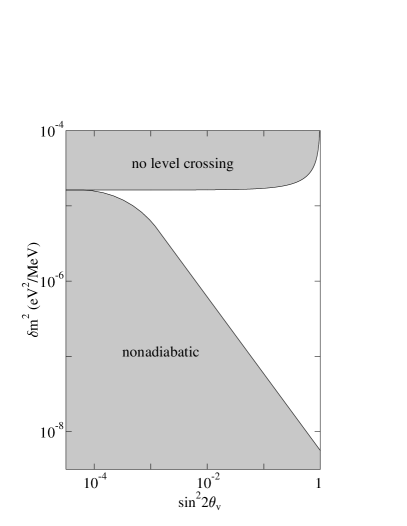
Figure 7: MSW conversion for a neutrino produced at the sun’s center. The upper shaded region indicates those $\delta m^{2}/E$ where the vacuum mass splitting is too great to be overcome by the solar density. Thus no level crossing occurs. The lower shaded region defines the region where the level crossing is non-adiabatic ($\gamma_{c}$ less than unity). The unshaded region corresponds to adiabatic level crossings where strong $\nu_{e}\rightarrow\nu_{\mu}$ will occur.

One can envision superimposing on fig. 7 the spectrum of solar neutrinos, plotted as a function of ${\delta m^{2}\over E}$ for some choice of $\delta m^{2}$. Since Davis sees some solar neutrinos, the solutions must correspond to the boundaries of the triangle in fig. 7. The horizontal boundary indicates the maximum ${\delta m^{2}\over E}$ for which the sun’s central density is sufficient to cause a level crossing. If a spectrum properly straddles this boundary, we obtain a result consistent with the Homestake experiment in which low energy neutrinos (large 1/E) lie above the level-crossing boundary (and thus remain $\nu_{e}$’s), but the high-energy neutrinos (small 1/E) fall within the unshaded region where strong conversion takes place. Thus such a solution would mimic nonstandard solar models in that only the ⁸B neutrino flux would be strongly suppressed. The diagonal boundary separates the adiabatic and non-adiabatic regions. If the spectrum straddles this boundary, we obtain a second solution in which low energy neutrinos lie within the conversion region, but the high-energy neutrinos (small 1/E) lie below the conversion region and are characterized by $\gamma\ll 1$ at the crossing density. (Of course, the boundary is not a sharp one, but is characterized by the Landau-Zener exponential). Such a non-adiabatic solution is quite distinctive since the flux of pp neutrinos, which is strongly constrained in the standard solar model and in any steady-state nonstandard model by the solar luminosity, would now be sharply reduced. Finally, one can imagine “hybrid” solutions where the spectrum straddles both the level-crossing (horizontal) boundary and the adiabaticity (diagonal) boundary for small $\theta$, thereby reducing the ⁷Be neutrino flux more than either the pp or ⁸B fluxes.

Figure 8: Illustration of the SMA, LMA, and LOW solutions arising out of fits to the event rates for Cl, Kamiokande, and SAGE/GALLEX. Figure provided by K. Heeger.

What are the results of a careful search for MSW solutions satisfying the Homestake, Kamiokande, and SAGE/GALLEX constraints? This was explored in detail by several groups (see fig. 8). One solution, corresponding to a region surrounding $\delta m^{2}\sim 6\cdot 10^{-6}$eV² and $\sin^{2}2\theta_{v}\sim 6\cdot 10^{-3}$, is the hybrid case described above. It is commonly called the small-mixing-angle solution (SMA). A second, large-angle solution (LMA) corresponds to $\delta m^{2}\sim 10^{-5}$eV² and $\sin^{2}2\theta_{v}\sim$ 0.6. These solutions can be distinguished by their characteristic distortions of the solar neutrino spectrum. The survival probabilities $P_{\nu_{e}}^{\rm MSW}$(E) for the small- and large-angle parameters given above are shown as a function of E in fig. 9.

Figure 9: MSW survival probabilities P(E_ν) for typical small angle and large angle solutions.

The MSW mechanism provides a natural explanation for the pattern of observed solar neutrino fluxes. While it requires profound new physics, both massive neutrinos and neutrino mixing are expected in extended models.

2.6 SuperKamiokande, SNO, and the Neutrino Mixing Matrix

Over the past five years the Cl/SAGE/GALLEX/Kamiokande hints of new neutrino physics have been spectacularly confirmed by SuperKamiokande and SNO, and a program to further constrain the neutrino mass matrix with terrestrial neutrino experiments has been inaugurated by KamLAND and K2K.

SuperKamiokande and Sudbury Neutrino Observatory (SNO) detectors are real-time counting detectors, in contrast to the radiochemical detectors such as Homestake, GALLEX/GNO, and SAGE, which can only determine a time- and energy-integral of the flux. Both SuperKamiokande and SNO can detect neutrinos through elastic scattering

$$\nu_{x}+e^{-}\rightarrow\nu_{x}+e^{-}.$$ (47)

The electrons coming from this reaction are confined to a forward cone, with most of the observed spread in angles around the forward peak coming from the limited angular resolution of the detector. To an excellent approximation the recorded events (including the effects of resolution) are contained in the forward hemisphere. Thus experimentalist can use the isotropic distribution of events in the backward hemisphere (defined around the vector pointing from the sun) to determine the background, then substract in the forward hemisphere to obtain the events coming from solar neutrinos. The neutrino energy is difficult to reconstruct because the initial neutrino momentum is shared by the scattered neutrino and electron. Nevertheless, for MSW solutions like the SMA where there is a significant distortion of the $\nu_{e}$ spectrum, there is a sufficient residual distortion of the electron spectrum to signal new physics. The SuperKamiokande collaboration carefully calibrated the detector with electrons from a linac so that small spectral distortions could be reliably extracted.

In addition to the reaction eq. (47) SNO can detect neutrinos by two additional reactions, one via the charged current

$$\nu_{e}+\mathrm{d}\rightarrow\mathrm{p}+\mathrm{p}+e^{-},$$ (48)

and the second via neutral current scattering

$$\nu_{x}(\overline{\nu}_{x})+\mathrm{d}\rightarrow\nu_{x}(\overline{\nu}_{x})+\mathrm{p}+\mathrm{n}.$$ (49)

The neutrons produced in eq. (49) can be detected either by (n,$\gamma)$ on the heavy water or on a salt introduced to enhance the capture, or by using ³He proportional counters. The electrons coming from the reaction (48) are quite hard, with energies not too different from $\sim E_{\nu}-1.44$ MeV, and with a angular distribution approximately that of a pure GT transition in the relativistic limit, ($1-\cos\theta_{e}/3$) with respect to the incident neutrino. This backward peaking contrasts nicely with the forward-peaked elastic scattering signal.

The hardness of the charged current reaction (eq. (48)) makes it an effective tool for finding spectral distortions induced by the MSW mechanism. The SNO spectral distortion expect for the SMA solution ($\delta m^{2}\sim 5\times 10^{-6}$ eV² and $\sin 2\theta\sim 0.01$) is shown in fig. 10.

Figure 10: The dashed line shows the spectrum distortion at SNO for the small-angle MSW solution ($\delta m^{2}\sim 5\times 10^{-6}$ eV² and $\sin 2\theta\sim 0.01$). The solid line is the spectrum without MSW oscillations, normalized to the same total rate as with MSW oscillations.

If there are no oscillations into sterile states (new neutrino states lacking the usual standard model weak interactions), the neutral current reaction (eq. (49)) measures the total SSM flux, independent of flavor. One other reaction of potential interest

$$\bar{\nu}_{e}+\mathrm{d}\rightarrow\mathrm{n}+\mathrm{n}+e^{+}$$ (50)

produces a two-neutron coincidence. Electron antineutrinos can arise from spin-flavor oscillations [26, 27] in the sun and, of course, from supernovae.

As the solar neutrino problem deepened with the new measurements from SAGE/GALLEX and Kamiokande, a second neutrino anomaly also began to draw attention. Several early underground detectors (IMB, Kamiokande, and later Soudan II) found a deficit of muons produced by atmospheric neutrinos. Atmospheric neutrinos arise from the decay of secondary pions, kaons, and muons produced by the collisions of primary cosmic rays with the oxygen and nitrogen nuclei in the upper atmosphere. For energies less than 1 GeV all the secondaries decay :

$$\pi^{\pm}(K^{\pm}) \rightarrow \mu^{\pm}+\nu_{\mu}(\overline{\nu}_{\mu}),$$

$$\mu^{\pm} \rightarrow e^{\pm}+\nu_{e}(\overline{\nu}_{e})+\overline{\nu}_{\mu}(\nu_{\mu}).$$ (51)

Consequently one expects the ratio

$$r=(\nu_{e}+\overline{\nu}_{e})/(\nu_{\mu}+\overline{\nu}_{\mu})$$ (52)

to be approximately 0.5 in this energy range. Detailed Monte Carlo calculations [28], including the effects of muon polarization, give $r\sim 0.45$. As one is evaluating a ratio of similarly calculated processes, $r$ does not require an absolute flux calculation and is thus relative free of systematic uncertainties. Different groups estimating this ratio, even though they start with neutrino fluxes which can differ in magnitude by up to 25%, all agree within a few percent [29]. As the shower energy increases more muons survive due to time dilation. Hence one expects the ratio $r$ to decrease as the energy increases. The ratio (observed to predicted) of ratios

$$R={(\nu_{\mu}/\nu_{e})_{\rm data}\over(\nu_{\mu}/\nu_{e})_{\rm MonteCarlo}}$$ (53)

studied by the experimentalists should then be unity, in the absence of oscillations.

The first “smoking gun” for neutrino oscillations came from the detailed atmospheric $\nu$ results of SuperKamiokande. The initial announcement of neutrino oscillations, made in 1998, is now supported by 1489 days of data. The experimenters found

$$R=0.638\pm 0.016({\rm stat})\pm 0.050({\rm syst})$$

for sub-GeV events which were fully contained in the detector and

$$R=0.658^{+0.030}_{-0.028}({\rm stat})\pm 0.078({\rm syst})$$

for fully- and partially-contained multi-GeV events. The large deviation from $R=1$ indicates neutrino oscillations. Much more dramatic evidence for oscillations comes from measuring $R$ as a function of the zenith angle, $\Theta$, between the vertical and incident neutrino. A down-going neutrino ($\Theta\sim 0^{o}$) travels through the atmosphere above the detector (a distance of about 20 km), whereas an up-going neutrino ($\Theta\sim 180^{o}$) has traveled through the entire Earth (a distance of about 13000 km). Hence a measurement of the flux as a function of the zenith angle yields information about neutrino survival probabilities as a function of the distance traveled.

Figure 11: The ratio of fully contained events measured at SuperKamiokande versus reconstructed $L/E_{\nu}$. The dashed lines show the expected shape for $\nu_{\mu}\leftrightarrow\nu_{\tau}$ oscillations with $\delta m^{2}=2.2\cdot 10^{-3}$ eV² and $\sin^{2}2\theta=1$.

The SuperKamiokande collaboration measured the zenith angle dependence not only of $R$, but also of the electron and muon neutrino fluxes separately [9]. This information is shown in Fig. 11, where the data is plotted as a function of the reconstructed $L/E_{\nu}$ instead of the zenith angle. The data exhibit a zenith-angle (distance) dependent deficit of muon neutrinos, but not of electron neutrinos, a behavior consistent with $\nu_{\mu}\rightarrow\nu_{\tau}$ oscillations. This interpretation is consistent with the deficits of up-going muons measured with the Kamiokande [30] and MACRO [31] detectors. These muons are produced by the very high energy up-going muon neutrinos in the rock surrounding the detectors.

One remarkable feature of the SuperKamiokande atmospheric neutrino results is the deduced mixing angle. Designating the two mass eigenstates participating in the mixing as 2 and 3, the best fit $\sin^{2}2\theta_{23}$ is 1, with $\sin^{2}\theta_{23}\geq 0.92$ at 90% c.l. As quark mixing angles are small, a $\nu$ mixing angle near maximal ($\theta_{23}\sim 45^{\circ}$) was not anticipated. The best-fit $\delta m^{2}_{23}$ is $\sim 2.5\cdot 10^{-3}$ eV².

This year an equally spectacularly resolution of the solar neutrino problem was obtained by SNO. SNO’s proof of oscillations was definitive: the heavy-flavor neutrinos produced as a result of solar $\nu_{e}$ oscillations were seen directly, by comparing the charge current and neutral current results.

SNO’s initial results are shown in fig. 12. The detector’s three $\nu$ channels – charge and neutral current scattering off deuterium and $\nu$-electron elastic scattering – combine to show that approximately two-thirds of the solar flux is in heavy flavors. The fluxes deduced, assuming a standard ⁸B $\nu$ spectrum shape, are [8]

$$\phi_{\nu_{e}}=(1.76\pm 0.05(stat)\pm 0.09(syst))\cdot 10^{6}/\mathrm{cm}^{2}\mathrm{s}$$

$$\phi_{\nu_{heavy}}=(3.41\pm 0.45(stat){}^{+0.48}_{-0.45}(syst))\cdot 10^{6}/\mathrm{cm}^{2}\mathrm{s}.$$ (54)

The 5.3 $\sigma$ difference is the significance of the oscillation proof. The total active flux, measured above the neutron breakup threshold for deuterium of 2.2 MeV, is

$$\phi_{\nu}=5.09^{+0.44}_{-0.43}(stat){}^{+0.46}_{-0.43})\cdot 10^{6}/\mathrm{cm}^{2}\mathrm{s}$$ (55)

in excellent agreement with SSM results.

Furthermore the results point to a unique solution in the MSW plane, the LMA solution, with a best fit $\delta m^{2}\sim 5\cdot 10^{-5}$ eV² and $\sin^{2}2\theta\sim 0.75$. Thus the oscillation corresponds to a new $\delta m^{2}$, distinct from the atmospheric $\nu$ solution, and while the oscillation appears to be not quite maximal, the mixing angle is again large. For three light neutrinos, we can label this mixing as that between mass eigenstates 1 and 2 with $\theta_{12}\sim 30^{\circ}$.

Figure 12: The ⁸B solar neutrino flux decomposed into electron and heavy-flavor components. The diagonal bands show the total flux measured by the SNO neutral-current reaction (solid) and predicted by the SSM (dashed). The intersection with charge-current and neutral current bands determines the flavor content. From Ref. [8].

Figure 13: Allowed regions of the MSW plane consistent with the SNO day and night energy spectra, the results from the Cl and SAGE/GALLEX/GNO experiments, and the day and night spectra from SuperKamiokande. The star indicates the best fit. Only the LMA region is allowed at 99% c.l. From Ref. [32].

The SuperKamiokande and SNO determinations of $\theta_{23}$ and $\theta_{12}$ are an exciting and important step in defining the neutrino mixing matrix, a quantity we hope will point the way to the next standard model. The three-flavor neutrino mixing matrix is conventionally written as

$$\left(\begin{array}[]{c}\nu_{e}\\ \nu_{\mu}\\ \nu_{\tau}\end{array}\right) = \left(\begin{array}[]{ccc}c_{12}c_{13}&s_{12}c_{13}&s_{13}e^{-i\delta}\\ -s_{12}c_{23}-c_{12}s_{23}s_{13}e^{i\delta}&c_{12}c_{23}-s_{12}s_{23}s_{13}e^{i\delta}&s_{23}c_{13}\\ s_{12}s_{23}-c_{12}c_{23}s_{13}e^{i\delta}&-c_{12}s_{23}-s_{12}c_{23}s_{13}e^{i\delta}&c_{23}c_{13}\end{array}\right)\left(\begin{array}[]{c}\nu_{1}\\ \nu_{2}\\ \nu_{3}\end{array}\right)$$ (65)

$$= \left(\begin{array}[]{ccc}1&&\\ &c_{23}&s_{23}\\ &-s_{23}&c_{23}\end{array}\right)\left(\begin{array}[]{ccc}c_{13}&&s_{13}e^{-i\delta}\\ &1&\\ -s_{13}e^{i\delta}&&c_{13}\end{array}\right)\left(\begin{array}[]{ccc}c_{12}&s_{12}&\\ -s_{12}&c_{12}&\\ &&1\end{array}\right)\left(\begin{array}[]{c}\nu_{1}\\ \nu_{2}\\ \nu_{3}\end{array}\right)$$ (78)

Here $c_{12}=\cos\theta_{12}$, etc. Despite the discoveries of the past five years, we have yet to complete this matrix. Mixing between eigenstates 1 and 3 has not yet measured: disappearance results from the Chooz [33] and Palo Verde [34] reactor experiments limit $\theta_{13}\mathrel{\hbox to0.0pt{\lower 4.0pt\hbox{\hskip 1.0pt$\sim$}\hss}\raise 1.0pt\hbox{$<$}}10^{\circ}$ in the atmospheric $\delta m^{2}$ range. Furthermore there is great interest in measuring CP violation effects, due to the large mixing angles so far measured and to the possibility that the baryon number asymmetry arises through leptogenesis. CP violation in oscillations requires a nonvanishing $\sin\theta_{13}$ in addition to $\delta$. Several very long baseline oscillation proposals have been made in which CP-violation would be disentangled from matter effects and from various neutrino parameter uncertainties.

Recently two important laboratory neutrino oscillation results have added to our picture of the mixing matrix. The atmospheric neutrino $\delta m^{2}$ range has been tested in the K2K experiment, in which events initiated by $\sim$ 1 GeV $\nu_{\mu}$s produced by the KEK proton synchrontron are recorded in SuperKamiokande [35]. The null hypothesis of no oscillations is allowed only at a confidence level $\mathrel{\hbox to0.0pt{\lower 4.0pt\hbox{\hskip 1.0pt$\sim$}\hss}\raise 1.0pt\hbox{$<$}}0.007$. The best-fit oscillation parameters, $\delta m^{2}\sim 2.7\cdot 10^{-3}$ eV² and $\sin^{2}2\theta\sim 1$, are in excellent agreement with the atmospheric neutrino values. The current data represents about half of the beam time expected for the experiment.

Very recently KamLAND, the first terrestrial experiment to probe the solar $\delta m^{2}$ range, announced initial results [36]. This long-baseline experiment records reactor $\bar{\nu}_{e}$ events in a liquid scintillator detector built at the site that once housed Kamiokande. Initial results confirm oscillations at 99.95% c.l., rule out all two-flavor solar neutrino solutions other than LMA, and significantly narrow the range of allowed $\delta m_{12}^{2}$ when combined with the solar neutrino results. The KamLAND results are shown in fig. 14. Ultimately results from KamLAND combined with a high-precision measurement of solar pp neutrinos could determine both $\delta m_{12}^{2}$ and $\sin^{2}2\theta_{12}$ with increased accuracy.

Figure 14: Two-neutrino oscillation constraints from KamLAND superimposed on the solar neutrino LMA allowed region. From Ref. [36].

Important question remain about the masses as well. All of the oscillation results test mass differences. Thus the absolute scale of $\nu$ mass must be probed in other experiments, such as tritium $\beta$ decay. The current limit from the Mainz and Troitsk experiments is $m_{\bar{\nu}_{e}}\mathrel{\hbox to0.0pt{\lower 4.0pt\hbox{\hskip 1.0pt$\sim$}\hss}\raise 1.0pt\hbox{$<$}}2.2$ eV [37]. As results from large-scale structure surveys now underway will be affected by $\nu$ masses as small as 0.3 eV, further progress must be made in direct $\nu$ mass experiments to eliminate a potentially significant cosmological uncertainty.

We do not know the mass hierarchy. Both normal (the solar neutrino mass pair light) and inverted (this pair heavy) are allowed by the data.

We do not know the charge conjugation properties of neutrinos. Neutrinos are unique among standard model fermions in allowing both Dirac and Majorana mass terms, as was noted earlier in the discussion of the seesaw mechanism. These mass terms can be distinguished because Majorana masses break lepton number conservation, allowing neutrinoless $\beta\beta$ decay to take place. Several recent next-generation $\beta\beta$ decay proposals argue that current lifetime limits can be improved by factors of $\sim$ 100, yielding sensitivities to Majorana masses of 10-50 milli-eV. Many mass scenarios consistent with the solar and atmospheric neutrino results predict neutrinoless $\beta\beta$ decay at this level.

Thus we are a very exciting juncture. We have found the first evidence for physics beyond the standard model, and we know this physics has immediate consequences beyond nuclear and particle physics, affecting particle dark matter, large-scale structure, and baryogenesis. The discoveries coming from astrophysical neutrinos are stimulating ambitious new experiments with both terrestrial and astrophysical beams. A great deal of information remains hidden and yet is accessible to the next generation of experiments, experiments that will require new neutrino beams and long-baseline megadetectors, as well as high sensitive instruments for measuring double beta decay and probing the low-energy portion of the solar neutrino flux. There are many reasons to hope that these endeavors will provide an experimental foundation for constructing the next standard model of subatomic physics.

3 Supernovae, Supernova Neutrinos, and Nucleosynthesis

Consider a massive star, in excess of 10 solar masses, burning the hydrogen in its core under the conditions of hydrostatic equilibrium. When the hydrogen is exhausted, the core contracts until the density and temperature are reached where 3$\alpha\rightarrow^{12}$C can take place. The He is then burned to exhaustion. This pattern (fuel exhaustion, contraction, and ignition of the ashes of the previous burning cycle) repeats several times, leading finally to the explosive burning of ²⁸Si to Fe. For a heavy star, the evolution is rapid: the star has to work harder to maintain itself against its own gravity, and therefore consumes its fuel faster. A 25 solar mass star would go through all of these cycles in about 7 My, with the final explosive Si burning stage taking a few days. The result is an “onion skin” structure of the pre-collapse star in which the star’s history can be read by looking at the surface inward: there are concentric shells of H, ⁴He, ¹²C, ¹⁶O and ²⁰Ne, and ²⁸Si, with Fe at the center.

3.1 The Explosion Mechanism [38]

The source of energy for this evolution is nuclear binding energy. A plot of the nuclear binding energy $\delta$ as a function of nuclear mass shows that the minimum is achieved at Fe. In a scale where the ¹²C mass is picked as zero:

¹²C     $\delta$/nucleon = 0.000 MeV

¹⁶O     $\delta$/nucleon = -0.296 MeV

²⁸Si    $\delta$/nucleon = -0.768 MeV

⁴⁰Ca    $\delta$/nucleon = -0.871 MeV

⁵⁶Fe    $\delta$/nucleon = -1.082 MeV

⁷²Ge    $\delta$/nucleon = -1.008 MeV

⁹⁸Mo    $\delta$/nucleon = -0.899 Mev

Once the Si burns to produce Fe, there is no further source of nuclear energy adequate to support the star. So as the last remnants of nuclear burning take place, the core is largely supported by degeneracy pressure, with the energy generation rate in the core being less than the stellar luminosity. The core density is about 2 $\times 10^{9}$ g/cc and the temperature is kT $\sim$ 0.5 MeV.

Thus the collapse that begins with the end of Si burning is not halted by a new burning stage, but continues. As gravity does work on the matter, the collapse leads to a rapid heating and compression of the matter. As the nucleons in Fe are bound by about 8 MeV, sufficient heating can release $\alpha$s and a few nucleons. At the same time, the electron chemical potential is increasing. This makes electron capture on nuclei and any free protons favorable,

$$e^{-}+p\rightarrow\nu_{e}+n.$$ (79)

Note that the chemical equilibrium condition is

$$\mu_{e}+\mu_{p}=\mu_{n}+\langle E_{\nu}\rangle.$$ (80)

Thus the fact that neutrinos are not trapped plus the rise in the electron Fermi surface as the density increases, lead to increased neutronization of the matter. The escaping neutrinos carry off energy and lepton number. Both the electron capture and the nuclear excitation and disassociation take energy out of the electron gas, which is the star’s only source of support. This means that the collapse is very rapid. Numerical simulations find that the iron core of the star ($\sim$ 1.2-1.5 solar masses) collapses at about 0.6 of the free fall velocity.

In the early stages of the infall the $\nu_{e}$s readily escape. But neutrinos are trapped when a density of $\sim$ 10¹²g/cm³ is reached. At this point the neutrinos begin to scatter off the matter through both charged current and coherent neutral current processes. The neutral current neutrino scattering off nuclei is particularly important, as the scattering cross section is off the total nuclear weak charge, which is approximately the neutron number. This process transfers very little energy because the mass energy of the nucleus is so much greater than the typical energy of the neutrinos. But momentum is exchanged. Thus the neutrino “random walks” out of the star. When the neutrino mean free path becomes sufficiently short, the “trapping time” of the neutrino begins to exceed the time scale for the collapse to be completed. This occurs at a density of about 10¹² g/cm³, or somewhat less than 1% of nuclear density. After this point, the energy released by further gravitational collapse and the star’s remaining lepton number are trapped within the star.

If we take a neutron star of 1.4 solar masses and a radius of 10 km, an estimate of its binding energy is

$${GM^{2}\over 2R}\sim 2.5\times 10^{53}\mathrm{ergs}.$$ (81)

Thus this is roughly the trapped energy that later will be radiated in neutrinos.

The trapped lepton fraction $Y_{L}$ is a crucial parameter in the explosion physics: a higher trapped $Y_{L}$ leads to a larger homologous core, a stronger shock wave, and easier passage of the shock wave through the outer core, as will be discussed below. Most of the lepton number loss of an infalling mass element occurs as it passes through a narrow range of densities just before trapping. The reasons for this are relatively simple: on dimensional grounds weak rates in a plasma go as $T^{5}$, where T is the temperature. Thus the electron capture rapidly turns on due to heating of the matter as it falls toward the trapping radius, and lepton number loss is maximal just prior to trapping. Inelastic neutrino reactions have an important effect on these losses, as the coherent trapping cross section goes as $E_{\nu}^{2}$ and is thus least effective for the lowest energy neutrinos. As these neutrinos escape, inelastic reactions repopulate the low energy states, allowing the neutrino emission to continue.

The velocity of sound in matter rises with increasing density. The inner homologous core, with a mass $M_{HC}\sim 0.6-0.9$ solar masses, is that part of the iron core where the sound velocity exceeds the infall velocity. In this subsonic central region any pressure variations that may develop in the homologous core during infall can smooth out before the collapse is completed. As a result, the homologous core collapses as a unit, retaining its density profile. That is, if nothing were to happen to prevent it, the homologous core would collapse to a point.

The collapse of the homologous core continues until nuclear densities are reached. As nuclear matter is rather incompressible ($\sim$ 200 MeV/f³), the nuclear equation of state is effective in halting the collapse: maximum densities of 3-4 times nuclear are reached, e.g., perhaps $6\cdot 10^{14}$ g/cm³. The innermost shell of matter reaches this supernuclear density first, rebounds, sending a pressure wave out through the homologous core. This wave travels faster than the infalling matter, as the homologous core is characterized by a sound speed in excess of the infall speed. Subsequent shells follow. The resulting series of pressure waves collect near the sonic point (the edge of the homologous core). As this point reaches nuclear density and comes to rest, a shock wave breaks out and begins its traversal of the outer core.

Initially the shock wave may carry an order of magnitude more energy than is needed to eject the mantle of the star (less than 10⁵¹ ergs). But as the shock wave travels through the outer iron core, it heats and melts the iron that crosses the shock front, at a loss of $\sim$ 8 MeV/nucleon. The enhanced electron capture that occurs off the free protons left in the wake of the shock, coupled with the sudden reduction of the neutrino opacity of the matter (recall $\sigma_{coherent}\sim N^{2}$), greatly accelerates neutrino emission. This is another energy loss. The summed losses from shock wave heating and neutrino emission are comparable to the initial energy carried by the shock wave. Thus most numerical models fail to produce a successful “prompt” hydrodynamic explosion: the shock stalls before it reaches the outer mantle.

Most of the attention in the past decade focused on two explosion scenarios. In the prompt mechanism described above, the shock wave is sufficiently strong to survive the passage of the outer iron core with enough energy to blow off the mantle of the star. The most favorable results were achieved with smaller stars (less than 15 solar masses) where there is less overlying iron, and with soft equations of state, which produce a more compact neutron star and thus lead to more energy release. In part because of the lepton number loss problems discussed earlier, now it is widely believed that this mechanism fails for all but unrealistically soft nuclear equations of state.

The delayed mechanism begins with a failed hydrodynamic explosion; after about 0.01 seconds the shock wave stalls at a radius of 200-300 km. It exists in a sort of equilibrium, gaining energy from matter falling across the shock front, but losing energy to the heating of that material. However, after perhaps 0.5 seconds, the shock wave is revived due to neutrino heating of the nucleon “soup” left in the wake of the shock. This heating comes primarily from charged current reactions off the nucleons in that nucleon gas; quasi-elastic scattering also contributes. This high entropy radiation-dominated gas may reach two MeV in temperature. The pressure exerted by this gas helps to push the shock outward. It is important to note that there are limits to how effective this neutrino energy transfer can be: if matter is too far from the core, the coupling to neutrinos is too weak to deposit significant energy. If too close, the matter may be at a temperature (or soon reach a temperature) where neutrino emission cools the matter as fast or faster than neutrino absorption heats it. The term “gain radius” is used to describe the region where useful heating is done.

This subject is still controversial and unclear. The problem is numerically challenging, forcing modelers to handle the difficult hydrodynamics of a shock wave; the complications of the nuclear equation of state at densities not yet accessible to experiment; modeling in two or three dimensions; handling the slow diffusion of neutrinos; etc. Not all of these aspects can be handled reasonably at the same time, even with existing supercomputers. Thus there is considerable disagreement about whether we have any supernova model that succeeds in ejecting the mantle.

However the explosion proceeds, there is agreement that 99% of the 3 $\cdot 10^{53}$ ergs released in the collapse is radiated in neutrinos of all flavors. The time scale over which the trapped neutrinos leak out of the protoneutron star is about three seconds. Through most of their migration out of the protoneutron star, the neutrinos are in flavor equilibrium

$$\mathrm{e.g.},~{}~{}\nu_{e}+\bar{\nu}_{e}\leftrightarrow\nu_{\mu}+\bar{\nu}_{\mu}.$$ (82)

As a result, there is an approximate equipartition of energy among the neutrino flavors. After weak decoupling, the $\nu_{e}$s and $\bar{\nu_{e}}$s remain in equilibrium with the matter for a longer period than their heavy-flavor counterparts, due to the larger cross sections for scattering off electrons and because of the charge-current reactions

$$\nu_{e}+\mathrm{n} \leftrightarrow\mathrm{p}+e^{-}$$

$$\bar{\nu_{e}}+\mathrm{p} \leftrightarrow\mathrm{n}+e^{+}.$$ (83)

Thus the heavy flavor neutrinos decouple from deeper within the star, where temperatures are higher. Typical calculations yield

$$T_{\nu_{\mu}}\sim T_{\nu_{\tau}}\sim 8\mathrm{MeV}~{}~{}~{}~{}T_{\nu_{e}}\sim 3.5\mathrm{MeV}~{}~{}~{}~{}T_{\bar{\nu_{e}}}\sim 4.5\mathrm{MeV}.$$ (84)

The difference between the $\nu_{e}$ and $\bar{\nu_{e}}$ temperatures is a result of the neutron richness of the matter, which enhances the rate for charge-current reactions of the $\nu_{e}$s, thereby keeping them coupled to the matter somewhat longer. (This temperature hierarchy, particular the difference between the heavy-flavor and electron neutrino temperatures, is still a matter of some debate, as it is influenced by both the explosion mechanism (e.g., by neutron fingers and other types of mixing) and the detailed modeling of the microphysics. Some recent work [39] argues for considerably smaller temperature differences than those given above.)

This temperature hierarchy is important because temperature inversions are a potential signature of oscillations. A three-flavor MSW level-crossing diagram is shown in fig. 15. Naively (that is, without considering neutrino-neutrino scattering and other effects that could alter this picture) the crossings corresponding to $\delta m^{2}_{solar}$ and $\delta m^{2}_{atmos}$ both occur well outside the neutrino sphere, that is, after the neutrinos have decoupled and have fixed spectra characterized by the temperatures given above. (For example, $\delta m^{2}_{atmos}$ corresponds to a electron density typical of the base of the carbon zone, prior to the explosion.) Thus a $\nu_{e}\leftrightarrow\nu_{\tau}$ oscillation would produce a distinctive $T\sim 8$ MeV spectrum of $\nu_{e}$s. Because neutrino-nucleus cross sections often grow as a high power of the neutrino energy (due both to phase space and threshold effects), this will produce elevated $\nu_{e}$ event rates in many detectors. Oscillations may also have an effect on nucleosynthesis, such as the $\nu$-process we will discuss below.

Figure 15: Three-flavor neutrino level-crossing diagram. The illustrated $\nu_{e}\leftrightarrow\nu_{\mu}$ and $\nu_{e}\leftrightarrow\nu_{\tau}$ crossings should arise from the solar and atmospheric $\delta m^{2}$s. The diagram illustrates that these crossing occur outside the neutrinosphere, in regions where the neutrinos are fully decoupled from the matter.

3.2 The Neutrino Process [40]

Core-collapse supernovae are one of the major engines driving galactic chemical evolution, producing and ejecting the metals that enrich our galaxy. The discussion of the previous section described the hydrostatic evolution of a presupernova star in which large quantities of the most abundant metals (C, O, Ne,…) are synthesized and later ejected during the explosion. During the passage of the shock wave through the star’s mantle, temperature of $\sim(1-3)\cdot 10^{9}$K and are reached in the silicon, oxygen, and neon shells. This shock wave heating induces $(\gamma,\alpha)\leftrightarrow(\alpha,\gamma)$ and related reactions that generate a mass flow toward highly bound nuclei, resulting in the synthesis of iron peak elements as well as less abundant odd-A species. Rapid neutron-induced reactions are thought to take place in the high-entropy atmosphere just above the mass cut, producing about half of the heavy elements above A $\sim$ 80. Finally, the $\nu$-process described below is responsible for the synthesis of rare species such as ¹¹B and ¹⁹F. This process involves the weak response of nuclei at momentum transfers where the allowed approximation is no longer valid. Thus we will use the $\nu$-process in this section to illustrate some of the relevant nuclear physics.

One of the problems – still controversial – that may be connected with the neutrino process is the origin of the light elements Be, B and Li, elements which are not produced in sufficient amounts in the big bang or in any of the stellar mechanisms we have discussed. The traditional explanation has been cosmic ray spallation interactions with C, O, and N in the interstellar medium. In this picture, cosmic ray protons collide with C at relatively high energy, knocking the nucleus apart. So in the debris one can find nuclei like ¹⁰B, ¹¹B, and ⁷Li.

But there are some problems with this picture. First of all, this is an example of a secondary mechanism: the interstellar medium must be enriched in the C, O, and N to provide the targets for these reactions. Thus cosmic ray spallation must become more effective as the galaxy ages. The abundance of boron, for example, would tend to grow quadratically with metallicity, since the rate of production goes linearly with metallicity. But observations, especially recent measurements with the HST, find a linear growth [41] in the boron abundance.

A second problem is that the spectrum of cosmic ray protons peaks near 1 GeV, leading to roughly comparable production of the two isotopes ¹⁰B and ¹¹B. That is, while it takes more energy to knock two nucleons out of carbon than one, this difference is not significant compared to typical cosmic ray energies. More careful studies lead to the expectation that the abundance ratio of ¹¹B to ¹⁰B might be $\sim$ 2. In nature, it is greater than 4.

Fans of cosmic ray spallation have offered solutions to these problems, e.g., similar reactions occurring in the atmospheres of nebulae involving lower energy cosmic rays. As this suggestion was originally stimulated by the observation of nuclear $\gamma$ rays from Orion, now retracted, some of the motivation for this scenario has evaporated. Here we focus on an alternative explanation, synthesis via neutrino spallation.

Previously we described the allowed Gamow-Teller (spin-flip) and Fermi weak interaction operators. These are the appropriate operators when one probes the nucleus at a wavelength – that is, at a size scale – where the nucleus responds like an elementary particle. We can then characterize its response by its macroscopic quantum numbers, the spin and charge. On the other hand, the nucleus is a composite object and, therefore, if it is probed at shorter length scales, all kinds of interesting radial excitations will result, analogous to the vibrations of a drumhead. For a reaction like neutrino scattering off a nucleus, the full operator involves the additional factor

$$e^{i\vec{k}\cdot\vec{r}}\sim 1+i\vec{k}\cdot\vec{r}$$ (85)

where the expression on the right is valid if the magnitude of $\vec{k}$ is not too large. Thus the full charge operator includes a “first forbidden” term

$$\sum_{i=1}^{A}\vec{r}_{i}\tau_{3}(i)$$ (86)

and similarly for the spin operator

$$\sum_{i=1}^{A}[\vec{r}_{i}\otimes\vec{\sigma}(i)]_{J=0,1,2}\tau_{3}(i).$$ (87)

These operators generate collective radial excitations, leading to the so-called “giant resonance” excitations in nuclei. The giant resonances are typically at an excitation energy of 20-25 MeV in light nuclei. One important property is that these operators satisfy a sum rule (Thomas-Reiche-Kuhn) of the form

$$\sum_{f}|\langle f|\sum_{i=1}^{A}r(i)\tau_{3}(i)|i\rangle|^{2}\sim{NZ\over A}\sim{A\over 4}$$ (88)

where the sum extends over a complete set of final nuclear states. These first-forbidden operators tend to dominate the cross sections for scattering the high energy supernova neutrinos ($\nu_{\mu}$s and $\nu_{\tau}$s), with $E_{\nu}\sim$ 25 MeV, off light nuclei. From the sum rule above, it follows that nuclear cross sections per target nucleon are roughly constant.

The E1 giant dipole mode described above is depicted qualitatively in fig. 16a. This description, which corresponds to an early model of the giant resonance response by Goldhaber and Teller, involves the harmonic oscillation of the proton and neutron fluids against one another. The restoring force for small displacements would be linear in the displacement and dependent on the nuclear symmetry energy. There is a natural extension of this model to weak interactions, where axial excitations occur. For example, one can envision a mode similar to that of fig. 16a where the spin-up neutrons and spin-down protons oscillate against spin-down neutrons and spin-up protons, the spin-isospin mode of fig. 16b. This mode is one that arises in a simple SU(4) extension of the Goldhaber-Teller model, derived by assuming that the nuclear force is spin and isospin independent, at the same excitation energy as the E1 mode. In full, the Goldhaber-Teller model predicts a degenerate 15-dimensional supermultiplet of giant resonances, each obeying sum rules analogous to the TRK sum rule. While more sophisticated descriptions of the giant resonance region are available, of course, this crude picture is qualitatively accurate.

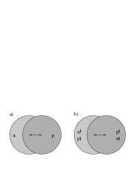
Figure 16: Schematic illustration of a) the E1 giant dipole mode familiar from electromagnetic interactions and b) a spin-isospin giant dipole mode associated with the first-forbidden weak axial response.

This nuclear physics is important to the $\nu$-process. The simplest example of $\nu$-process nucleosynthesis involves the Ne shell in a supernova. Because of the first-forbidden contributions, the cross section for inelastic neutrino scattering to the giant resonances in Ne is $\sim 3\cdot 10^{-41}$ cm²/flavor for the more energetic heavy-flavor neutrinos. This reaction

$$\nu+A\rightarrow\nu^{\prime}+A^{*}$$ (89)

transfers an energy typical of giant resonances, $\sim$ 20 MeV. A supernova releases about 3 $\times 10^{53}$ ergs in neutrinos, which converts to about $4\times 10^{57}$ heavy flavor neutrinos. The Ne shell in a 20 M_⊙ star has at a radius $\sim$ 20,000 km. Thus the neutrino fluence through the Ne shell is

$$\phi\sim{4\cdot 10^{57}\over 4\pi(20,000\mathrm{km})^{2}}\sim 10^{38}/\mathrm{cm}^{2}.$$ (90)

Thus folding the fluence and cross section, one concludes that approximately 1/300th of the Ne nuclei interact.

This is quite interesting since the astrophysical origin of ¹⁹F had not been understood. The only stable isotope of fluorine, ¹⁹F has an abundance

$${{}^{19}\mathrm{F}\over{}^{20}\mathrm{Ne}}\sim{1\over 3100}.$$ (91)

This leads to the conclusion that the fluorine found in a tube of toothpaste was created by neutral current neutrino reactions deep inside some ancient supernova.

The calculation of the final ¹⁹F/²⁰Ne ratio is more complicated than the simple 1/300 ratio given above:
$\bullet$ When Ne is excited by $\sim$ 20 MeV through inelastic neutrino scattering, it breaks up in two ways

$${}^{20}\mathrm{Ne}(\nu,\nu^{\prime})^{20}\mathrm{Ne}^{*} \rightarrow^{19}\mathrm{Ne}+n\rightarrow^{19}\mathrm{F}+e^{+}+\nu_{e}+n$$

$${}^{20}\mathrm{Ne}(\nu,\nu^{\prime})^{20}\mathrm{Ne}^{*} \rightarrow^{19}\mathrm{F}+p$$ (92)

with the first reaction occurring half as frequently as the second. As both channels lead to ¹⁹F, we have correctly estimated the instantaneous abundance ratio in the Ne shell of

$${{}^{19}\mathrm{F}\over{}^{20}\mathrm{Ne}}\sim{1\over 300}.$$ (93)

$\bullet$ We must also address the issue of whether the produced ¹⁹F survives. In the first 10^-8 sec the co-produced neutrons in the first reaction react via

$${}^{15}\mathrm{O}(n,p)^{15}\mathrm{N}~{}~{}^{19}\mathrm{Ne}(n,\alpha)^{16}\mathrm{O}~{}~{}^{20}\mathrm{Ne}(n,\gamma)^{21}\mathrm{Ne}~{}~{}^{19}\mathrm{Ne}(n,p)^{19}\mathrm{F}$$ (94)

with the result that about 70% of the ¹⁹F produced via spallation of neutrons is then immediate destroyed, primarily by the $(n,\alpha)$ reaction above. In the next $10^{-6}$ sec the co-produced protons are also processed

$${}^{15}\mathrm{N}(p,\alpha)^{12}\mathrm{C}~{}~{}^{19}\mathrm{F}(p,\alpha)^{16}\mathrm{O}~{}~{}^{23}\mathrm{Na}(p,\alpha)^{20}\mathrm{Ne}$$ (95)

with the latter two reactions competing as the primary proton poisons. This makes an important prediction: stars with high Na abundances should make more F, as the ²³Na acts as a proton poison to preserve the produced F. $\bullet$ Finally, there is one other destruction mechanism, the heating associated with the passage of the shock wave. It turns out the the F produced prior to shock wave passage can survive if it is in the outside half of the Ne shell. The reaction

$${}^{19}\mathrm{F}(\gamma,\alpha)^{15}\mathrm{N}$$ (96)

destroys F for peak explosion temperatures exceeding $1.7\cdot 10^{9}$K. Such a temperature is produced at the inner edge of the Ne shell by the shock wave heating, but not at the outer edge.

If all of this physics in handled is a careful network code that includes the shock wave heating and F production both before and after shock wave passage, the following are the results:

$$\begin{array}[]{cc}\underline{[^{19}\mathrm{F}/^{20}\mathrm{Ne}]/[^{19}\mathrm{F}/^{20}\mathrm{Ne}]_{\odot}}&\underline{T_{\mathrm{heavy}~{}\nu}\mathrm{(MeV)}}\\ 0.14&4\\ 0.6&6\\ 1.2&8\\ 1.1&10\\ 1.1&12\end{array}$$

where the abundance ratio in the first column has been normalized to the solar value. One sees that the attribution of F to the neutrino process argues that the heavy flavor $\nu$ temperature must be greater than 6 MeV, a result theory favors. One also sees that F cannot be overproduced by this mechanism: although the instantaneous production of F continues to grow rapidly with the neutrino temperature, too much F results in its destruction through the $(p,\alpha)$ reaction, given the metalicity assumed in this calculation (a solar abundance of the competing proton poison ²³Na). Indeed, this illustrates an odd quirk: although in most cases the neutrino process is a primary mechanism, one needs ²³Na present to produce significant F. Thus in this case the neutrino process is a secondary mechanism.

While there are other significant neutrino process products (⁷Li, ¹³⁸La, ¹⁸⁰Ta, ¹⁵N …), the most important product is ¹¹B, produced by spallation off carbon. A calculation by Timmes et al.[41] found that the combination of the neutrino process, cosmic ray spallation and big-bang nucleosynthesis together can explain the evolution of the light elements. The neutrino process, which produces a great deal of ¹¹B but relatively little ¹⁰B, combines with the cosmic ray spallation mechanism to yield the observed isotope ratio. Again, one prediction of this picture is that early stars should be ¹¹B rich, as the neutrino process is primary and operates early in our galaxy’s history; the cosmic ray production of ¹⁰B is more recent. There is hope that HST studies will soon be able to discriminate between ¹⁰B and ¹¹B: as yet this has not been done.

3.3 The $r$-process [42]

Beyond the iron peak nuclear Coulomb barriers become so high that charged particle reactions become ineffective, leaving neutron capture as the mechanism responsible for producing the heaviest nuclei. If the neutron abundance is modest, this capture occurs in such a way that each newly synthesized nucleus has the opportunity to $\beta$ decay, if it is energetically favorable to do so. Thus weak equilibrium is maintained within the nucleus, so that synthesis is along the path of stable nuclei. This is called the s- or slow-process. However a plot of the s-process in the (N,Z) plane reveals that this path misses many stable, neutron-rich nuclei that are known to exist in nature. This suggests that another mechanism is at work, too. Furthermore, the abundance peaks found in nature near masses A $\sim$ 130 and A $\sim$ 190, which mark the closed neutron shells where neutron capture rates and $\beta$ decay rates are slower, each split into two sub-peaks. One set of sub-peaks corresponds to the closed-neutron-shell numbers N $\sim$ 82 and N $\sim$ 126, and is clearly associated with the s-process. The other set is shifted to smaller N, $\sim$ 76 and $\sim$ 116, respectively, and is suggestive of a much more explosive neutron capture environment where neutron capture can be rapid.

This second process is the r- or rapid-process, characterized by:
$\bullet$ The neutron capture is fast compared to $\beta$ decay rates.
$\bullet$ The equilibrium maintained within a nucleus is established by (n$,\gamma)\leftrightarrow(\gamma,$n): neutron capture fills up the available bound levels in the nucleus until this equilibrium sets in. The new Fermi level depends on the temperature and the relative n$/\gamma$ abundance.
$\bullet$ The nucleosynthesis rate is thus controlled by the $\beta$ decay rate: each $\beta^{-}$ capture converting n $\rightarrow$ p opens up a hole in the neutron Fermi sea, allowing another neutron to be captured.
$\bullet$ The nucleosynthesis path is along exotic, neutron-rich nuclei that would be highly unstable under normal laboratory conditions.
$\bullet$ As the nucleosynthesis rate is controlled by the $\beta$ decay, mass will build up at nuclei where the $\beta$ decay rates are slow. It follows, if the neutron flux is reasonable steady over time so that equilibrated mass flow is reached, that the resulting abundances should be inversely proportional to these $\beta$ decay rates.

Let’s first explore the (n$,\gamma)\leftrightarrow(\gamma,$n) equilibrium condition, which requires that the rate for (n$,\gamma)$ balances that for $(\gamma,$n) for an average nucleus. So consider the formation cross section

$$A+\mathrm{n}\rightarrow(A+1)+\gamma.$$ (97)

This is an exothermic reaction, as the neutron drops into the nuclear well. Our averaged cross section, assuming a resonant reaction (the level density is high in heavy nuclei) is

$$\langle\sigma v\rangle_{(\mathrm{n},\gamma)}=\left({2\pi\over\mu kT}\right)^{3/2}{\Gamma_{\mathrm{n}}\Gamma_{\gamma}\over\Gamma}e^{-E/KT}$$ (98)

where E $\sim$ 0 is the resonance energy, and the $\Gamma$s are the indicated partial and total widths. Thus the rate per unit volume is

$$r_{(\mathrm{n},\gamma)}\sim N_{\mathrm{n}}N_{A}\left({2\pi\over\mu kT}\right)^{3/2}{\Gamma_{\mathrm{n}}\Gamma_{\gamma}\over\Gamma}$$ (99)

where $N_{\mathrm{n}}$ and $N_{A}$ are the neutron and nuclear number densities and $\mu$ the reduced mass. This has to be compared to the $(\gamma,$n) rate.

The $(\gamma,$n) reaction requires the photon number density in the gas. This is given by the Bose-Einstein distribution

$$N(\epsilon)={8\pi\over c^{3}h^{3}}{\epsilon^{2}d\epsilon\over e^{\epsilon/kT}-1}.$$ (100)

The high-energy tail of the normalized distribution can thus be written

$$\sim{1\over N_{\gamma}\pi^{2}}\epsilon^{2}e^{-\epsilon/kT}d\epsilon$$ (101)

where in the last expression we have set $\hbar=c=1$.

Now we need the resonant cross section in the $(\gamma,$n) direction. For photons the wave number is proportional to the energy, so

$$\sigma_{(\gamma,\mathrm{n})}={\pi\over\epsilon^{2}}{\Gamma_{\gamma}\Gamma_{\mathrm{n}}\over(\epsilon-E_{r})^{2}+(\Gamma/2)^{2}}.$$ (102)

As the velocity is c =1,

$$\langle\sigma v\rangle={1\over\pi^{2}N_{\gamma}}\int_{0}^{\infty}\epsilon^{2}e^{-\epsilon/kT}d\epsilon{\pi\over\epsilon^{2}}{\Gamma_{\gamma}\Gamma_{\mathrm{n}}\over(\epsilon-E_{r})^{2}+(\Gamma/2)^{2}}.$$ (103)

We evaluate this in the usual way for a sharp resonance, remembering that the energy integral over just the denominator above (the sharply varying part) is $2\pi/\Gamma$

$$\sim{\Gamma_{\gamma}\Gamma_{\mathrm{n}}\over N_{\gamma}}e^{-E_{r}/kT}{2\over\Gamma}.$$ (104)

So that the rate becomes

$$r_{(\gamma,\mathrm{n})}\sim 2N_{A+1}{\Gamma_{\gamma}\Gamma_{\mathrm{n}}\over\Gamma}e^{-E_{r}/kT}.$$ (105)

Equating the (n$,\gamma)$ and $(\gamma,$n) rates and taking $N_{A}\sim N_{A-1}$ then yields

$$N_{\mathrm{n}}\sim{2\over(\hbar c)^{3}}\left({\mu c^{2}kT\over 2\pi}\right)^{3/2}e^{-E_{r}/kT}$$ (106)

where the $\hbar$s and $c$s have been properly inserted to give the right dimensions. Now $E_{r}$ is essentially the binding energy. So plugging in the conditions $N_{\mathrm{n}}\sim 3\times 10^{23}$/cm³ and $T_{9}\sim 1$, we find that the binding energy is $\sim$ 2.4 MeV. Thus neutrons are bound by about 30 times $kT$, a value that is still small compared to a typical binding of 8 MeV for a normal nucleus. (In this calculation the neutron reduced mass is calculated by assuming a nuclear target with A=150.)

The above calculation fails to count spin states for the photons and nuclei and is thus not quite correct. But it makes the essential point: the $r$-process involves very exotic species largely unstudied in any terrestrial laboratory. It is good to bear this in mind, as in the following section we will discuss the responses of such nuclei to neutrinos. Such responses thus depend on the ability of theory to extrapolate responses from known nuclei to those quite unfamiliar.

The path of the $r$-process is along neutron-rich nuclei, where the neutron Fermi sea is just $\sim$ (2-3) MeV away from the neutron drip line (where no more bound neutron levels exist). After the $r$-process finishes (the neutron exposure ends) the nuclei decay back to the valley of stability by $\beta$ decay. This can involve some neutron spallation ($\beta$-delayed neutrons) that shift the mass number A to a lower value. But it certainly involves conversion of neutrons into protons, and that shifts the $r$-process peaks at N $\sim$ 82 and 126 to a lower N, off course. This effect is clearly seen in the abundance distribution: the $r$-process peaks are shifted to lower N relative to the s-process peaks. This is the origin of the second set of “sub-peaks” mentioned at the start of the section.

It is believed that the $r$-process can proceed to very heavy nuclei (A $\sim$ 270) where it is finally ended by $\beta$-delayed and n-induced fission, which feeds matter back into the process at an A $\sim$ A_max/2. Thus there may be important cycling effects in the upper half of the $r$-process distribution.

What is the site(s) of the $r$-process? This has been debated many years and still remains a controversial subject:
$\bullet$ The $r$-process requires exceptionally explosive conditions

$\rho$(n) $\sim 10^{20}$ cm^-3   T $\sim 10^{9}$K   t $\sim$ 1s.

$\bullet$ Both have been primary and secondary sites have been proposed. Primary sites are those not requiring preexisting metals. Secondary sites are those where the neutron capture occurs on preexisting s-process seeds.
$\bullet$ Suggested primary sites include the the neutronized atmosphere above the proto-neutron star in a Type II supernova, neutron-rich jets produced in supernova explosions or in neutron star mergers, inhomogeneous big bangs, etc.
$\bullet$ Secondary sites, where $\rho$(n) can be lower for successful synthesis, include the He and C zones in Type II supernovae, the red giant He flash, etc.

The balance of evidence favors a primary site, so one requiring no pre-enrichment of heavy s-process metals. Among the evidence:

1) Keck and HST studies of very-metal-poor halo stars: The most important evidence are the recent measurements of Cowan, Sneden et al. [43] of very metal-poor stars ([Fe/H] $\sim$ -1.7 to -3.12) where an $r$-process distribution very much like that of our sun has been seen for Z $\mathrel{\hbox to0.0pt{\lower 4.0pt\hbox{\hskip 1.0pt$\sim$}\hss}\raise 1.0pt\hbox{$>$}}$ 56. Furthermore, in these stars the iron content is variable. This suggests that the “time resolution” inherent in these old stars is short compared to galactic mixing times (otherwise Fe would be more constant). The conclusion is that the $r$-process material in these stars is most likely from one or a few local supernovae. The fact that the distributions match the solar $r$-process (at least above charge 56) strongly suggests that there is some kind of unique site for the high-Z portion of the $r$-process: the solar $r$-process distribution did not come from averaging over many different kinds of $r$-process events. Clearly the fact that these old stars are enriched in $r$-process metals also strongly argues for a primary process: the $r$-process works quite well in an environment where there are few initial s-process metals. (The situation for elements below Z=56 is somewhat different. While an adequate discussion would take us beyond the limits of these lectures, interested reader are directed to Ref. [42].)

2) There are also fairly good theoretical arguments that a primary $r$-process occurring in a core-collapse supernova might be viable [44]. First, galactic chemical evolution studies indicate that the growth of $r$-process elements in the galaxy is consistent with low-mass Type II supernovae in rate and distribution. More convincing is the fact that modelers have shown that the conditions needed for an $r$-process (very high neutron densities, temperatures of 1-3 billion degrees) might be realized in a supernova. The site is the last material expelled from the supernova, the matter just above the mass cut. When this material is blown off the star initially, it is a very hot neutron-rich, radiation-dominated gas containing neutrons and protons, but an excess of the neutrons. As it expands off the star and cools, the material first goes through a freeze-out to $\alpha$ particles, a step that essentially locks up all the protons in this way. Then the $\alpha$s interact through reactions like

$$\alpha+\alpha+\alpha \rightarrow{}^{12}\mathrm{C}$$

$$\alpha+\alpha+n \rightarrow{}^{9}\mathrm{Be}$$

to start forming heavier nuclei. Note, unlike the big bang, that the density is high enough to allow such three-body interactions to bridge the mass gaps at A = 5,8. The $\alpha$ capture continues up to heavy nuclei, to A $\sim$ 80, in the network calculations. The result is a small number of “seed” nuclei, a large number of $\alpha$s, and excess neutrons. These neutrons preferentially capture on the heavy seeds to produce an $r$-process. Of course, what is necessary is to have $\sim$ 100 excess neutrons per seed in order to successfully synthesize heavy mass nuclei. Some of the modelers find conditions where this almost happens.

There are some very nice aspects of this site: the amount of matter ejected is about 10${}^{-5}-10^{-6}$ solar masses, which is just about what is needed over the lifetime of the galaxy to give the integrated $r$-process metals we see, taking a reasonable supernova rate. But there are also a few problems, especially the fact that with calculated entropies in the nucleon soup above the proto-neutron star, neutron fractions appear to be too low to produce a successful A $\sim$ 190 peak. There is some interesting recent work invoking neutrino oscillations [45] to cure this problem: charge current reactions on free protons and neutrons determine the n/p ratio in the gas. This is discussed briefly in the next section.

The nuclear physics of the $r$-process tells us that the synthesis occurs when the nucleon soup is in the temperature range of (3-1) $\cdot 10^{9}$K, which, in the hot bubble $r$-process described above, corresponds to a freeze-out radius of (600-1000) km and a time $\sim$ 10 seconds after core collapse. The neutrino fluence after freeze-out (when the temperature has dropped below 10⁹K and the $r$-process stops) is then $\sim$ (0.045-0.015) $\cdot 10^{51}$ ergs/(100km). Thus, after completion of the $r$-process, the newly synthesized material experiences an intense flux of neutrinos. This brings up the question of whether the neutrino flux could have any effect on the $r$-process.

3.4 Neutrinos and the $r$-process [46]

Before describing the exotic effects of neutrino oscillations on the supernovae and nucleosynthesis, we will examine standard-model effects that are nevertheless quite interesting. The nuclear physics of this section – neutrino-induced neutron spallation reactions – is also relevant to recently proposed supernova neutrino observatories such as OMNIS and LAND. Comparing to our earlier discussion of carbon- and neon-zone synthesis by the $\nu$-process, it is apparent that neutrino effects could be much larger in the hot bubble $r$-process: the synthesis occurs much closer to the star than our Ne radius of 20,000 km: estimates are 600-1000 km. The $r$-process is completed in about 10 seconds (when the temperature drops to about one billion degrees), but the neutrino flux is still significant as the $r$-process freezes out. The net result is that the “post-processing” neutrino fluence - the fluence that can alter the nuclear distribution after the $r$-process is completed - is about 100 times larger than that responsible for fluorine production in the Ne zone. Recalling that 1/300 of the nuclei in the Ne zone interacted with neutrinos, and remembering that the relevant neutrino-nucleus cross sections scale as A, one quickly sees that the probability of a $r$-process nucleus interacting with the neutrino flux is approximately unity.

Because the hydrodynamic conditions of the $r$-process are highly uncertain, one way to attack this problem is to work backward in time. We know the final $r$-process distribution (what nature gives us) and we can calculate neutrino-nucleus interactions relatively well. Thus from the observed $r$-process distribution (including neutrino post-processing) we can work backward to find out what the $r$-process distribution looked like at the point of freeze-out. In Figs. 17 and 18, the “real” $r$-process distribution - that produced at freeze-out - is given by the dashed lines, while the solid lines show the effects of the neutrino post-processing for a particular choice of fluence. The nuclear physics input into these calculations is precisely that previously described: GT and first-forbidden cross sections, with the responses centered at excitation energies consistent with those found in ordinary, stable nuclei, taking into account the observed dependence on $|N-Z|$.

Figure 17: Comparison of the $r$-process distribution that would result from the freeze-out abundances near the A $\sim$ 130 mass peak (dashed line) to that where the effects of neutrino post-processing have been include (solid line). The fluence has been fixed by assuming that the A = 124-126 abundances are entirely due to the $\nu$-process.

One important aspect of the figures is that the mass shift is significant. This has to do with the fact that a 20 MeV excitation of a neutron-rich nucleus allows multiple neutrons ( $\sim$ 5) to be emitted. (Remember we found that the binding energy of the last neutron in an $r$-process neutron-rich nuclei was about 2-3 MeV under typical $r$-process conditions.) The second thing to notice is that the relative contribution of the neutrino process is particularly important in the “valleys” beneath the mass peaks: the reason is that the parents on the mass peak are abundant, and the valley daughters rare. In fact, it follows from this that the neutrino process effects can be dominant for precisely seven isotopes (Te, Re, etc.) lying in these valleys. Furthermore if an appropriate neutrino fluence is picked, these isotope abundances are produced perfectly (given the abundance errors). The fluences are

$$\mathrm{N} = 82~{}\mathrm{peak}~{}~{}~{}~{}~{}0.031\cdot 10^{51}\mathrm{ergs/(100km)^{2}/flavor}$$

$$\mathrm{N} = 126~{}\mathrm{peak}~{}~{}~{}~{}0.015\cdot 10^{51}\mathrm{ergs/(100km)^{2}/flavor},$$

values in fine agreement with those that would be found in a hot bubble $r$-process. So this is circumstantial but significant evidence that the material near the mass cut of a Type II supernova is the site of the $r$-process: there is a neutrino fingerprint.

Figure 18: As in fig. 17, but for the A $\sim$ 195 mass peak. The A = 183-187 abundances are entirely attributed to the $\nu$-process.

4 Neutrino Oscillation Constraints from the $r$-process

Many aspects of supernova physics could be altered by neutrino oscillations. One satisfying consequence of the recent solar and atmospheric neutrino oscillation discoveries is that the derived parameters, the mass differences and mixing angles, have begun to narrow some of “parameter space” for such supernova oscillation effects.

Earlier it was noted that understanding neutrino transport is an essential but highly nontrivial part of the supernova mechanism. The addition of neutrino oscillations adds another layer of complication, and thus opportunity for surprises. To set the stage for this discussion, we recall that the density at the neutrinosphere is $\sim 10^{12}$g cm^-3 and the density at the position of the stalled shock is [47] $\sim 2\times 10^{7}$ g cm^-3. Writing the MSW resonance density in appropriate units

$$\rho_{\rm res}=1.31\times 10^{6}\left({\delta m^{2}\over{\rm eV}^{2}}\right)\left({{\rm 10MeV}\over E_{\nu}}\right)\left({0.5\over{\rm Y}_{e}}\right)\cos 2\theta~{}~{}{\rm g}\>{\rm cm}^{-3},$$ (107)

one sees, for $E_{\nu}\sim 10$ MeV, that the range of $\delta m^{2}$s producing crossings between the neutrinosphere and the stalled shock wave is $\sim 1-10^{4}$ eV². Some time ago Fuller et al. [47] pointed out that $\nu_{e}-\nu_{heavy}$ oscillations in this region could substantial increase the explosion energy, as hot $\nu_{e}$s would couple more strongly to the matter because of the increase in the $\nu_{e}+n$ cross section (which goes as $E_{\nu}^{2}$, roughly). Unfortunately the necessary range of $\delta m^{2}$ includes neither the atmospheric nor solar values. Thus at least in the simplest scenario of three light neutrinos, the oscillations we know about from experiment may not affect this aspect of the explosion mechanism. (However there are many scenarios – a fourth neutrino motivated by LSND [48], CPT violation, etc – where this conclusion would need to be reexamined. Even in the simplest three-flavor scenario discussed above, one should consider complications that might move the MSW resonance position, such as the contributions of $\nu-\nu$ scattering to the MSW potential.)

The potential for neutrino oscillation to alter the $r$-process (if core-collapse supernovae are indeed the site) was also recognized some time ago. The $r$-process requires a neutron-rich environment: the ratio of electrons to baryons, $Y_{e}$, should be less than one half. $Y_{e}$ in the nucleosynthesis region is given approximately [49] by

$$Y_{e}\simeq{1\over 1+\lambda_{{\overline{\nu}}_{e}p}/\lambda_{\nu_{e}n}}\simeq{1\over 1+T_{{\overline{\nu}}_{e}}/T_{\nu_{e}}},$$ (108)

where $\lambda_{\nu_{e}n}$, etc. are the capture rates. Hence if $T_{{\overline{\nu}}_{e}}>T_{\nu_{e}}$, then the medium is neutron rich. But oscillations of the type $\nu_{e}\leftrightarrow\nu_{heavy}$ could invert this hierarchy, thus destroying a necessary condition for the $r$-process. In the simplest scenario of three light neutrinos and $\delta m^{2}$ consistent with the solar and atmospheric $\nu$ results, this catastrophe is avoided for the hot-bubble $r$-process because the crossings occur outside the region of interest. (However, the same caveats noted above apply.)

If the supernova is an $r$-process site it is also desirable to have a neutron to seed-nucleus ratio ${\ \lower-1.2pt\vbox{\hbox{\hbox to0.0pt{$>$\hss}\lower 5.0pt\vbox{\hbox{$\sim$}}}}\ }100$ in order that the heavier $r$-process species (i.e., those in the $A=195$ peak) can be produced. This ratio is basically determined by three quantities: i) the expansion rate; ii) the electron fraction $Y_{e}$; and iii) the entropy per baryon. Though different calculations [44, 50] disagree on the value of the entropy in the neutrino-driven wind during the $r$-process nucleosynthesis, several models can produce values of these three parameters adequate for a successful $r$-process – that is, until certain $\nu$ reactions are considered. These $\nu$ reactions, acting during or immediately after freezeout, allow too many seed nuclei to form, thus producing an unfavorable neutron/seed ratio. This prevents the $r$-process from synthesizing the heaviest nuclei, those in the $A\sim$ 190 peak. The worst of these $\nu$ reactions is called the alpha effect.

The alpha effect [51] occurs at the epoch of alpha particle formation. As the temperature drops, essentially all of the protons and most of the neutrons in the ejecta lock themselves into tightly bound alpha particles. As the matter was initially neutron rich, free neutrons remain and $Y_{e}$ is below 0.5. The alpha effect pushes the electron fraction higher, towards $Y_{e}=0.5$. The increase in $Y_{e}$ comes about because $\nu_{e}$s capture on neutrons, with the produced protons capturing more neutrons to produce $\alpha$s, thereby reducing the number of free neutrons available for the $r$-process [52]. This effect has been shown to be the biggest impediment to achieving an acceptable $r$-process yield [53]. Matter-enhanced neutrino oscillations between electron neutrinos and other active species worsen this problem, tending to increase electron neutrino energies and thus the average charge current cross section. On the other hand, active-sterile oscillations which diminish the flux of electron neutrinos outside some radius can reduce the alpha effect, and thus preserve the $r$-process. This scenario has been discussed extensively because sterile neutrinos may also account for the LSND results.

There is an important constraint on this “solution,” however. In models where the $r$-process material is blown off the protoneutron star by a neutrino wind, a large flux of electron neutrinos is essential to overcome the binding effects of gravity. As nucleons are gravitationally bound by about $\sim 100\,{\rm MeV}$ near the surface of the protoneutron star while each neutrino has an energy $\sim 10$ MeV, $\sim$ 10 charge-current $\nu$-nucleon interactions are needed to eject the nucleon to infinity. This in turn requires that the active-sterile oscillation occur at a relatively large radius, so that strong wind effects at smaller $r$ are unaffected. It proves possible to arrange the necessary condition through active-sterile $\nu_{e}\rightleftharpoons\nu_{s}$ and $\bar{\nu}_{e}\rightleftharpoons\bar{\nu}_{s}$ channels. In such a scheme [45] the lightest sterile neutrino would be heavier than the $\nu_{e}$ and split from it by a vacuum mass-squared difference of 3 eV${}^{2}{\ \lower-1.2pt\vbox{\hbox{\hbox to0.0pt{$<$\hss}\lower 5.0pt\vbox{\hbox{$\sim$}}}}\ }\delta m^{2}_{es}{\ \lower-1.2pt\vbox{\hbox{\hbox to0.0pt{$<$\hss}\lower 5.0pt\vbox{\hbox{$\sim$}}}}\ }$ 70 eV² with vacuum mixing angle $\sin^{2}2\theta_{es}>10^{-4}$. Whether this solution is necessary, though, is quite another matter. It has been argued that very fast expansion rates could circumvent the alpha effect by minimizing the $\nu$ fluence experienced by the matter. This underscores how difficult it is to assess our current understanding of the $r$-process when our theoretical models of supernovae seem to be less successful than Nature in producing explosions. (This reminds one that the foundation for our discoveries in solar neutrino physics was a reliable SSM!)

Finally, regardless of where the crossings occur within a supernova, the supernovae neutrinos that SNO, SuperKamiokande, and other detectors record will have been altered by oscillations, including potentially oscillation channels we have not yet probed elsewhere (e.g., $\theta_{13}$). The extent to which we can exploit neutrinos as a probe of supernova physics will depend on how well we succeed with current efforts to determine the entries in the mixing matrix.

This work was supported in part by the US Department of Energy under grants DE-FG03-00ER41132 and DE-FG02-01ER41187. Portions of these lectures were based on summer school notes prepared in collaboration with A. Baha Balantekin, whom I thank.

References

References

- [1] This section is an updated version of W. C. Haxton, Ann. Rev. Astron. Astrophys. 33, 459 (1995); the historical discussion is given in more detail in W. C. Haxton and B. R. Holstein, Am. J. Phys. 68, 15 (2000).
- [2] R. Davis, Jr., D. S. Harmer, and K. C. Hoffman, Phys. Rev. Lett. 20, 1205 (1966).
- [3] J. N. Abdurashitov et al., Phys. Lett. B 328, 234 (1994) and JETP 95, 181 (2002).
- [4] P. Anselmann et al., Phys. Lett. B 285, 376 (1992).
- [5] GNO Collaboration, M. Altmann et al., Phys. Lett. B 490, 16 (2002).
- [6] Y. Suzuki, Nucl. Phys. B 38, 54 (1995).
- [7] Y. Suzuki, talk presented at Neutrino ’98 (Takayama, Japan, June, 1998).
- [8] SNO Collaboration, Phys. Rev. Lett. 89, 011301 (2002) and Phys. Rev. Lett. 87, 071301 (2001).
- [9] Y. Fukuda et al. (Superkamiokande collaboration), Phys. Rev. Lett. 81, 1562 (1998); Phys. Lett. B 433, 9 (1998).
- [10] J. N. Bahcall, S. Basu, and M. H. Pinsonneault, Phys. Lett. B 433, 1 (1998) and Ap. J. 555, 990 (2001).
- [11] A. S. Brun, S. Turck-Chieze, and P. Morel, Ap. J. 506, 913 (1998) and private communication; S. Turck-Chieze and I. Lopez, Ap. J. 408, 347 (1993).
- [12] This section taken from W. C. Haxton, nucl-th/9901037.
- [13] K. Lande, talk presented at Neutrino ’98 (Takayama, Japan, June, 1998).
- [14] J. N. Bahcall, Neutrino Astrophysics, (Cambridge University, Cambridge, 1989).
- [15] S..Fukuda et al. (Superkamiokande Collaboration), Phys. Rev. Lett. 86, 5651 (2001); M. B. Smy, hep-ex/0208004/
- [16] J. N. Bahcall and R. Ulrich, Rev. Mod. Phys. 60, 297 (1988).
- [17] J. N. Bahcall and W. C. Haxton, Phys. Rev. D 40, 931 (1989).
- [18] V. Castellani, S. Degl’Innocenti, G. Fiorentini, M. Lissia, and B. Ricci, Phys. Rev. D 50, 4749 (1994).
- [19] K. M. Heeger and R. G. H. Robertson, Phys. Rev. Lett. 77, 3720 (1996).
- [20] J. Christensen-Dalsgaard, Lecture Notes on Stellar Oscillations, http://www.obs.aau.dk/j̃cd/oscilnotes/.
- [21] M. Gell-Mann, P. Ramond, and R. Slansky, in Supergravity, P. van Nieuwenhuizen and D.Z. Freedman, Eds., North Holland, Amsterdam, 1979, p. 315; T. Yanagida, in Proceedings of the Workshop on the Unified Theory and Baryon Number in the Universe, O. Sawada and A. Sugamoto, Eds., (KEK Report 79-18, 1979), p.95.
- [22] S. P. Mikheyev and A. Smirnov, Sov. J. Nucl. Phys. 42, 913 (1985); L. Wolfenstein, Phys. Rev. D 17, 2369 (1979).
- [23] H. Bethe, Phys. Rev. Lett. 56, 1305 (1986).
- [24] W. C. Haxton, Phys. Rev. Lett. 57, 1271 (1986).
- [25] S. J. Parke, Phys. Rev. Lett. 57, 1275 (1986).
- [26] C. S. Lim and W. J. Marciano, Phys. Rev. D 37, 1368 (1988).
- [27] E. Kh. Akhmedov, Sov. J. Nucl. Phys. 48, 382 (1988).
- [28] G. Barr, T.K. Gaisser, and T. Stanev, Phys. Rev. D 39, 3532 (1989); T.K. Gaisser, T. Stanev, and G. Barr, ibid. 38, 85 (1988).
- [29] H. Lee and S.A. Bludman, Phys. Rev. D 37, 122 (1988); E.V. Bugaev and V.A. Naumov, Phys. Lett. B 232, 391 (1989); M. Honda, K, Kasahara, K. Hidaka, and S. Midorikawa, Phys. Lett. B 248, 193 (1990); M. Kawasaki and S. Mizuta, Phys. Rev. D 43, 2900 (1991).
- [30] S. Hatakeyama et al. (Kamiokande collaboration), Phys. Rev. Lett. 81, 2016 (1998).
- [31] M. Ambrosio et al. (MACRO collaboration), Phys. Lett. B 434, 451 (1998).
- [32] A. W. P. Poon, hep-ex/0211013/
- [33] Chooz Collaboration, M. Apollonio et al., Phys. Lett. B 416, 415 (1999).
- [34] F. Boehm et al., Phys. Rev. D 64, 112001 (2001).
- [35] C. W. Walter, hep-ex/0211059/
- [36] KamLAND Collaboration, hep-ex/0212021/, to appear in Phys. Rev. Lett.
- [37] C. Weinheimer, hep-ex/0210050/
- [38] A. Mezzacappa et al., Ap. J. 495, 911 (1998); H.-Th. Janka and E. Muller, Astron. Astrophys. 306, 167 (1996); A. Burrows, S. Hayes, and B. A. Fryxell, Ap. J. 450, 830 (1995).
- [39] M. Th. Keil, G. G. Raffelt, and H.-T. Janka, astro-ph/0208035/ (submitted to Ap. J.)
- [40] S. E. Woosley and W. C. Haxton, Nature 334, 45 (1988); S. E. Woosley, D. H. Hartmann, R. D. Hoffman, and W. C. Haxton, Ap. J. 356, 272 (1990).
- [41] F. X. Timmes, S. E. Woosley, and T. A. Weaver, Ap. J. Suppl. 98, 617 (1995).
- [42] Y.-Z. Qian, to appear in Prog. Part. Nucl. Phys.
- [43] J. J. Cowan and C. Sneden, astro-ph/0212149/
- [44] S. E. Woosley, J. R. Wilson, G. J. Mathews, R. D. Hoffman, and B. S. Meyer, Ap. J. 433, 229 (1994).
- [45] G. C. McLaughlin, J.M. Fetter, A.B. Balantekin, and G. M. Fuller, Phys. Rev. C 59, 2873 (1999).
- [46] W. C. Haxton, K. Langanke, Y.-Z. Qian, and P. Vogel, Phys. Rev. Lett. 78, 2694 (1997) and Phys. Rev. C 55, 1532 (1997).
- [47] G.M. Fuller, R.W. Mayle, B.S. Meyer, and J.R. Wilson, Ap. J. 389, 517 (1992); R.W. Mayle, in Supernovae, A.G. Petschek, Ed., (Springer-Verlag, New York, 1990).
- [48] LSND Collaboration, Phys. Rev. Lett. 75, 2650 (1995); W. C. Louis, Nucl. Phys. B 91, 198 (2001); also see K. Eitel (KARMEN Collaboration), Contribution to the International Nuclear Physics Conference, Paris, August 1998.
- [49] Y.-Z. Qian et al., Phys. Rev. Lett. 71, 1965 (1993).
- [50] B.S. Meyer et al., Ap. J. 399, 656 (1992)); K. Takahashi,J. Witti, and H.-Th. Janka, Astron. Astrophys 286, 857 (1994).
- [51] B.S. Meyer, Ap. J. 449, L55 (1995).
- [52] G.M. Fuller and B.S. Meyer, Ap. J. 453, 792 (1995).
- [53] B. S. Meyer, G. C. McLaughlin, and G. M. Fuller, Phys. Rev. C 58, 3696 (1998).