Projection and ground state correlations made simple

Abstract

We develop and test efficient approximations to estimate ground state correlations associated with low- and zero-energy modes. The scheme is an extension of the generator-coordinate-method (GCM) within Gaussian overlap approximation (GOA). We show that GOA fails in non-Cartesian topologies and present a topologically correct generalization of GOA (topGOA). An RPA-like correction is derived as the small amplitude limit of topGOA, called topRPA. Using exactly solvable models, the topGOA and topRPA schemes are compared with conventional approaches (GCM-GOA, RPA, Lipkin-Nogami projection) for rotational-vibrational motion and for particle number projection. The results shows that the new schemes perform very well in all regimes of coupling.

I Introduction

Self-consistent mean-field models are nowadays the standard tool for nuclear structure calculations. Their quality has reached a level where one needs to take into account correlation effects beyond mean field, particularly those which are related to low-energy- or symmetry-modes. Typical examples are center-of-mass projection, particle-number projection, angular-momentum projection or quadrupole surface vibrations. There is a large variety of techniques to deal with those correlations, for a review see correlrev . The most widely used ones are the random phase approximation (RPA), see e.g. Rowe ; BB94 , and the generator coordinate method (GCM), see e.g. GCM ; heenenGCM . The latter has close links to projection formulae. The RPA has the advantage that it provides simple equations because it employs only second order commutators of the basic one-body operators with the Hamiltonian. However, it runs into difficulties with soft modes which arise typically near transition points. The GCM is very general and extremely robust, but also very cumbersome to handle. Thus one has developed simplifications in the aim to use also preferably second order expressions. This is achieved by the Gaussian overlap approximation (GOA) to GCM, for details see the review GCM . GCM-GOA is a fair compromise between the generality of GCM and the simplicity of RPA. It uses up to second order anti-commutators but can still deal with large amplitude collective motion. Second order approximation within the spirit of GOA have also been widely applied to projection schemes. The standard recipe $E_{\rm cm}=\langle\hat{P}_{\rm cm}^{2}\rangle/2mA$ for center of mass correction belongs to this class schmid . The similarly simple rotational correction $\langle\hat{J}^{2}\rangle/2\Theta$ has been widely employed, e.g. in the large scale fits of goriely . And there is the well known Lipkin-Nogami approach for particle-number projection Pra73a .

However, one has to be aware that the GOA is not always performing well. For example, it fails for rotational motion in weakly deformed systems and for particle number projection in the regime of weak pairing. The failure can be related to the topology of the collective coordinate under consideration. GOA is well suited for Cartesian coordinates which extend in the interval $(-\infty,+\infty)$ with constant volume element. The best example is here center of mass motion. But GOA is not necessarily appropriate for other topologies as, e.g., rotational motion whose coordinates are defined on a sphere. It can still work if the overlaps are falling off very quickly. But regimes of weak coupling have broad overlaps and thus the topology of the underlying coordinates is fully explored. It needs to be built in into the approximation. An example for rotational motion is found in rot . A most general construction for any topology is discussed in pom . The changes are, in fact, obvious and simple. It amounts to building the topology of the coordinates into the parameterization of the GOA. We call the emerging approach a topologically corrected Gaussian overlap approximation (topGOA).

It is the aim of this paper to investigate the accuracy of the topGOA for two cases most relevant in nuclear structure calculations, deformations and particle-number projection. We compare topGOA with RPA as well as full GCM and simple GOA. Furthermore, we derive a small amplitude limit of topGOA which gives at the end very simple and compact formulae for the collective ground-state correlations, in a sense comparable to RPA. We call that approach topRPA. In both test cases we employ a suitable generalization of the Lipkin-Meshkov-Glick model LMG .

II Conventional approaches

This section provides a brief summary of traditionally well known approaches for collective correlations, RPA and GCM up to GOA.

II.1 RPA correlations

The RPA theory is perhaps the most straightforward treatment of correlations beyond mean field theory. It gives the leading corrections in the limit of large number of interacting particles. With the RPA, one calculates an excitation spectrum of eigenfrequencies $\omega_{n}$ and the associated particle-hole operators $\hat{C}^{+}_{n}$ that generate the eigenmodes. These modes are also present in the RPA ground state as zero-point motion, leading to a RPA theory of the ground state correlation energy, see e.g. Rowe ; ring . For a single mode, the RPA correlation energy is given by

$$\Delta E=\frac{\omega}{2}\left(1-\langle\Phi_{0}|\{\hat{C},\hat{C}^{+}\}|\Phi_{0}\rangle\right)$$ (1)

where

$$\omega=\langle\Phi_{0}|[\hat{C},[\hat{H},\hat{C}^{+}]]|\Phi_{0}\rangle$$ (2)

and $|\Phi_{0}\rangle$ is the mean field ground state. In the case the mode corresponds to a broken continuous symmetry, $\omega=0$ and the formula should be applied by taking the $\omega\longrightarrow 0$ limit. It is also advantageous in that case to separate the generators into time-even and time-odd

$$\hat{Q}=\frac{1}{\sqrt{2}}\left(\hat{C}^{+}+\hat{C}\right)\quad,\quad\hat{P}=\frac{i}{\sqrt{2}}\left(\hat{C}^{+}-\hat{C}\right)\quad.$$ (3)

The $\hat{P}$ is usually the generator of a collective deformation, for example a center-of-mass shift in case of the translational mode. Particle-number projection is an example where the time-even operator $\hat{N}$ spans the collective space.

The RPA correlation energy (1) can fail due to double counting if one employs a sum over a large RPA spectrum fukuda64 , but double counting is negligible if only a few collective modes are used rowe68 . That is the line of approach followed here. For a most recent survey of RPA correlations along that line, see hagber . It will be taken up explicitly in the applications later on.

II.2 Generator coordinate method

II.2.1 General framework

The most general technique for constructing collective modes is the generator coordinate method (GCM). It utilizes a superposition of wave functions defined along some collective deformation path $\left\{|\Phi_{q}\rangle\equiv|q\rangle\right\}$. Each state $|q\rangle$ along this path is an independent particle state (or independent quasi-particle state in case of BCS). The correlated wave function is given by

$$|\Psi\rangle=\int dq\,|q\rangle\,f(q)\quad.$$ (4)

where the superposition function $f$ is determined by the Griffin-Hill-Wheeler equation

$$\int dq^{\prime}\,\left[{\cal H}(q,q^{\prime})-E{\cal I}(q,q^{\prime})\right]f(q^{\prime})=0\quad,$$ (5a)

$${\cal H}(q,q^{\prime})=\langle q|\hat{H}|{q^{\prime}}\rangle\quad,$$ (5b)

$${\cal I}(q,q^{\prime})=\langle q|{q^{\prime}}\rangle\quad.$$ (5c)

Normalizing $\Psi$, the correlation energy is given by

$$\Delta E=\langle\Psi|\hat{H}|\Psi\rangle-\langle\Phi_{0}|\hat{H}|\Phi_{0}\rangle$$ (6)

where $|\Phi_{0}\rangle\equiv|0\rangle$ is the ground state of the underlying independent particle model. The GCM can be easily generalized to multiple modes. One simply generalizes $q$ to a vector of deformations and extends $\int dq^{\prime}$ to a multi-dimensional integral, see e.g. JanSch ; brink68 ; GCM . The GCM is often applied in this straightforward, but tedious, manner where the overlaps and the solution of the Griffin-Hill-Wheeler equation are determined numerically, see e.g. Egi89a ; heenenGCM ; heenenGCM2 .

II.2.2 The Gaussian Overlap Approximation (GOA)

The full GCM is much more elaborate than RPA because one deals with the overlaps for any combination of $q$ and $q^{\prime}$ and the highly non-local Griffin-Hill-Wheeler equation. A dramatic simplification is achieved by the Gaussian overlap approximation (GOA). It represents the dependence of the overlaps on the difference $(q-q^{\prime})$ by a Gaussian times a polynomial in $(q-q^{\prime})^{n}$. The overlap is represented as a pure Gaussian,

$${\cal I}(q,q^{\prime})=\exp{\left(-\frac{\lambda}{4}(q-q^{\prime})^{2}\right)}\quad,$$ (7)

with

$$\lambda(\bar{q})=\frac{1}{2}\left(i\partial_{q}-i\partial_{q^{\prime}}\right)^{2}{\cal I}(q,q^{\prime})\Big{|}_{q=q^{\prime}=\bar{q}}\quad,$$ (8)

One usually goes up to second order derivatives in the expression for the Hamiltonian

$$\frac{{\cal H}(q,q^{\prime})}{{\cal I}(q,q^{\prime})} = {\cal H}_{0}(\bar{q})-\frac{1}{8}(q-q^{\prime})^{2}{\cal H}_{2}(\bar{q})\quad,$$ (9a)

$${\cal H}_{0}(\bar{q}) = {\cal H}(\bar{q},\bar{q})\quad,$$ (9b)

$${\cal H}_{2}(\bar{q}) = \left(i\partial_{q}-i\partial_{q^{\prime}}\right)^{2}\left.\frac{{\cal H}(q,q^{\prime})}{{\cal I}(q,q^{\prime})}\right|_{q=q^{\prime}=\bar{q}}\quad,$$ (9c)

$$\bar{q} = \frac{q+q^{\prime}}{2}\quad.$$ (9d)

For further details, see GCM . The GOA yields a dramatic simplification of the Griffin-Hill-Wheeler equation. Assuming that the coefficients depend only weakly on $\bar{q}$, one can recast the Griffin-Hill-Wheeler equation into a collective Schrödinger equation with a simple second derivative as operator for the kinetic energy. Large amplitudes in average collective deformation $\bar{q}=(q+q^{\prime})/2$ are still allowed. Thus the GCM-GOA is applicable to conditions of large fluctuation as are typical for low-energy modes and for symmetry projection.

A further dramatic simplification emerges if one restricts the considerations to small amplitudes also in $\bar{q}=(q+q^{\prime})/2$. Then collective dynamics becomes harmonic and all expressions can be worked out analytically. The final result is then just the RPA JanSch ; rowe68 ; brink68 . The correlations from GCM-GOA become then identical to the RPA correlations as given the above subsection II.1.

II.2.3 Beyond GOA

However, the GOA has its limitations. The Gaussian ansatz assumes tacitly that the collective coordinate spans the interval

$$q\in(-\infty,+\infty)\quad.$$ (10)

In other words, the dynamics is fundamentally Cartesian in the collective coordinates. This is certainly true for some situations, e.g. the center-of-mass motion where each coordinate $R_{x}$, $R_{y}$, and $R_{z}$ runs over $(-\infty,+\infty)$. But the presupposition is violated in many cases. In particular, in rotational motion the rotation angles are restricted to finite intervals with periodic boundary conditions. For such situations the GOA can be generalized by modifying the the arguments of the Gaussian to correctly include the topology of the collective mode rot ; pom . We call this generalization the topological GOA (topGOA). The details of topGOA depend, of course, on the actual mode under considerations. In the following, we exemplify and test topGOA for two typical and most important applications in nuclear physics: deformations and particle-number projection. The projection is straightforward and yields immediately expressions in second order throughout. The efficient treatment of deformations remains an important problem in nuclear structure. The theory should provide accurate correlation energies, going from the small-amplitude vibrational limit to the large amplitude static deformations and including the soft region in between. These applications will serve as a critical testing ground for the topRPA, and the small amplitude approximation to topGOA.

III Vibrations and rotational projection

III.1 The three-level model

The usual two-level Lipkin-Meshkov-Glick Hamiltonian has been widely used to model the collective motion of in a deformation coordinate, as it contains the vibrational and static deformation limits with the mean-field phase transition in between. However, the model does not have a continuous symmetry, which is an important aspect of the deformations. To include a continuous symmetry, we have extended the space in the Lipkin-Meskov-Glick model to three levels, and call the extended model the three-level model. Two of the levels are degenerate in the three-level, and the interactions treats those levels identically. This introduces a symmetry mode with the topology of rotations in a plane. For clarity we repeat here the definition of the three-level model; for details see hagber . The three levels are labelled 0,1, and 2. The basic $1ph$ transitions $0\!\rightarrow\!1$ are induced by $\hat{K}_{+,1}$ and those to state 2 by $\hat{K}_{+,2}$. The amount of excitation is measured by $\hat{K}_{0,i}\,,\,i\in\{1,2\}$. The $\hat{K}$ operators obey a quasi-spin algebra. The Hamiltonian of the model reads

$$\hat{H} = \epsilon\sum_{i=1}^{2}\hat{K}_{0,i}-\chi\frac{\epsilon}{2(N-1)}\sum_{i}(\hat{K}_{+,i}^{2}+\hat{K}_{-,i}^{2})\quad,$$ (11a)

$$\hat{K}_{0,i} = \sum_{m=1}^{N}\alpha_{im}^{+}\alpha_{im}^{\mbox{}}\quad,$$ (11b)

$$\hat{K}_{+,i} = \sum_{m=1}^{N}a_{im}^{+}a_{0m}^{\mbox{}}\quad,$$ (11c)

$$\hat{K}_{-,i} = \sum_{m=1}^{N}a_{0m}^{+}a_{im}^{\mbox{}}\quad.$$ (11d)

The exact solution of this Hamiltonian is obtained by diagonalization in the space of $\hat{K}_{x}^{n}\hat{K}_{y}^{m}$. The three-level Hamiltonian is the first term in eq. (11a). It defines the energetic relations amongst the levels. Note that the two excited states $i=1,2$ are degenerate. This gives the model the rotational symmetry. The second term in (11a) models a two-body interaction. It is again symmetric in $i=1\leftrightarrow 2$ which maintains rotational symmetry. The strength is regulated by $\chi$, defined to be dimensionless coupling strength. We will see later that $\chi\sim 1$ is the critical point in the model separating weak and string coupling.

It is convenient to analyze the many-particle wave function in terms of collective variables $\alpha$ and $\beta$. The collective wave function is defined

$$|\alpha\beta\rangle=e^{\tan(\alpha)\hat{K}_{+}(\beta)}|0\rangle{\cal N}^{-1/2}(\alpha)\quad,$$ (12)

where

$$\hat{K}_{+}(\beta)=\cos(\beta)\hat{K}_{+,1}+\sin(\beta)\hat{K}_{+,2}\quad,$$ (13)

and the normalization is given by

$${\cal N}(\alpha)=\langle 0|e^{\tan(\alpha)\hat{K}_{-}}e^{\tan(\alpha)\hat{K}_{+}}|0\rangle=\cos^{-2N}(\alpha)\quad.$$ (14)

Note that the model is rotationally invariant in the angle $\beta$. The motion in $\alpha$ corresponds to collective vibrations. The system is close to a good vibrator for small residual interaction, $\chi<1$. It is a rigid rotator for large $\chi>1$. The transitional regime $\chi\sim 1$ explores collective motion with large amplitude fluctuations. Two subtle details need to be mentioned: First, there is only one rotational degree-of-freedom which means that the model corresponds to rotations in a plane. Second, the vibrational degree-of-freedom contains relevant information only in the interval $\alpha\in\{0,\pi\}$, similar to the vibrational mode in the usual Lipkin-Meshkov-Glick model. This is the price one pays to have a simple model.

The simplicity of the model allows one to write down the exact overlaps analytically:

$${\cal I}(\alpha\beta,\alpha^{\prime}\beta^{\prime}) = {\left[\cos(\alpha)\cos(\alpha^{\prime})+\sin(\alpha)\sin(\alpha^{\prime})\cos(\beta\!-\!\beta^{\prime})\right]^{N}}\quad,$$ (15a)

$$\frac{{\cal H}(\alpha\beta,\alpha^{\prime}\beta^{\prime})}{{\cal I}(\alpha\beta,\alpha^{\prime}\beta^{\prime})} = N\epsilon\,\frac{\sin\alpha\sin\alpha^{\prime}\cos(\beta-\beta^{\prime})}{\cos\alpha\cos\alpha^{\prime}+\sin\alpha\sin\alpha^{\prime}\cos(\beta-\beta^{\prime})}-\chi\frac{\epsilon}{2}N\,\frac{\sin^{2}\alpha\cos^{2}\alpha^{\prime}+\cos^{2}\alpha\sin^{2}\alpha^{\prime}}{(\cos\alpha\cos\alpha^{\prime}+\sin\alpha\sin\alpha^{\prime}\cos(\beta-\beta^{\prime}))^{2}}\quad.$$ (15b)

The Hartree-Fock (HF) solution is obtained simply by minimizing the expectation value of the Hamiltonian in a state $|\alpha\beta\rangle$,

$$E_{\rm mf}(\alpha) = {\cal H}(\alpha\beta,\alpha\beta)$$ (16)

$$= N\epsilon\sin^{2}(\alpha)-\chi\epsilon N\sin^{2}(\alpha)\cos^{2}(\alpha)\quad.$$

with respect to the deformation $\alpha$,$\beta$. This yields the Hartree-Fock energy as $E_{\rm HF}=E_{\rm mf}(\alpha_{\rm HF})$ where the deformation of the minimum is denoted by $\alpha_{\rm HF}$. Note that the energy is independent of the actual value of $\beta$ due to rotational invariance of the three-level model.

III.2 The RPA modes

Small amplitude motion around the HF minimum induces collective excitations of the system. They can be worked out analytically for the three-level model hagber . There are two collective modes to be considered. At spherical shape $\alpha_{\rm HF}\sim 0$, there are two degenerate vibrational modes. The degeneracy is lifted with increasing $\alpha_{\rm HF}$. With further increasing $\alpha_{\rm HF}$, there comes a critical point where the RPA solutions become unstable. A different scenario develops after the transition point. The two modes separate into a rotational mode along $\beta$ and a vibrational mode along $\alpha$. The two eigenfrequencies are $\omega=0$, associated with the rotational mode, and $\omega=\epsilon\sqrt{\chi^{2}-1}$ for vibrations. Having these two modes at hand, one can compute the RPA correlation energy applying eq. (1) for each mode separately and add up the result to the total correlations.

III.3 The topGOA for the three-level model

The standard GOA overlaps can be obtained by expanding eq. (15) with respect to $(\alpha-\alpha^{\prime})$ and $(\beta-\beta^{\prime})$ up to the second order. We exemplify it here for the norm kernel at $\alpha=\alpha^{\prime}$ and expansion in $\beta-\beta^{\prime}$. GOA reads

$${\cal I}(\alpha\beta,\alpha\beta^{\prime}) = {\left[\cos^{2}(\alpha)+\sin^{2}(\alpha)\cos(\beta\!-\!\beta^{\prime})\right]^{N}},$$

$$= \left[1-2\sin^{2}(\alpha)\sin^{2}\left(\frac{\beta-\beta^{\prime}}{2}\right)\right]^{N},$$

$$\longrightarrow \exp\left(-\frac{N}{2}\sin^{2}(\alpha)(\beta-\beta^{\prime})^{2}\right).$$

The problem is obvious: the exact overlap is periodic in $\beta-\beta^{\prime}$ while the GOA is not.

To develop an appropriate ansatz for topGOA we have to look at the topology of the collective coordinates. The pair of coordinates $(\alpha,\beta)$ extends over the surface of the unit sphere. The exact overlaps (15) hint already the combinations of coordinates which is generated by this topology: $\cos(\alpha)\cos(\alpha^{\prime})+\sin(\alpha)\sin(\alpha^{\prime})\cos(\beta\!-\!\beta^{\prime})$. It is the measure for a distance on the sphere. The idea of topGOA is to apply to the norm overlap the Gaussian limit theorem for the shape of the overlap function while preserving the topological combination of the arguments. Similar combinations are to be used for expanding the Hamiltonian overlap. This yields then for the three-level model the form

$${\cal I}(\alpha\beta,\alpha^{\prime}\beta^{\prime}) = e^{-\frac{\lambda_{\alpha}}{4}\sin^{2}\left(\frac{\alpha\!-\!\alpha^{\prime}}{2}\right)-\frac{\lambda_{\beta}}{4}{\cal S}_{\alpha}\sin^{2}\left(\frac{\beta\!-\!\beta^{\prime}}{2}\right)}\;,$$ (17a)

$$\lambda_{\alpha} = \frac{1}{2}\left(i\partial_{\alpha}-i\partial_{\alpha^{\prime}}\right)^{2}{\cal I}(\alpha\beta,\alpha^{\prime}\beta)\Big{|}_{\alpha=\alpha^{\prime}=\bar{\alpha}}$$ (17b)

$$\lambda_{\beta}{\cal S}_{\alpha} = \frac{1}{2}\left(i\partial_{\beta}-i\partial_{\beta^{\prime}}\right)^{2}{\cal I}(\alpha\beta,\alpha\beta^{\prime})\Big{|}_{\beta=\beta^{\prime}=\bar{\beta}}$$ (17c)

$$\frac{{\cal H}(\alpha\beta,\alpha^{\prime}\beta^{\prime})}{{\cal I}(\alpha\beta,\alpha^{\prime}\beta^{\prime})} = {\cal H}_{0}-{\cal H}_{2}^{\alpha}\sin^{2}\left(\frac{\alpha\!-\!\alpha^{\prime}}{2}\right)$$ (17d)

$$-{\cal H}_{2}^{\beta}{\cal S}_{\alpha}\sin^{2}\left(\frac{\beta\!-\!\beta^{\prime}}{2}\right)\quad,$$

$${\cal H}_{0} = {\cal H}(\bar{\alpha}\bar{\beta},\bar{\alpha}\bar{\beta})$$ (17e)

$${\cal H}_{2}^{\alpha} = \frac{-1}{2}\left(\partial_{\alpha}\!-\!\partial_{\alpha^{\prime}}\right)^{2}\left.\frac{{\cal H}(\alpha\beta,\alpha^{\prime}\beta)}{{\cal I}(\alpha\beta,\alpha^{\prime}\beta)}\right|_{\alpha=\alpha^{\prime}=\bar{\alpha}}$$ (17f)

$${\cal H}_{2}^{\beta} = \frac{-1}{2{\cal S}_{\alpha}}\left.\left(\partial_{\beta}\!-\!\partial_{\beta^{\prime}}\right)^{2}\frac{{\cal H}(\alpha\beta,\alpha\beta^{\prime})}{{\cal I}(\alpha\beta,\alpha\beta^{\prime})}\right|_{\beta=\beta^{\prime}=\bar{\beta}}$$ (17g)

$${\cal S}_{\alpha} = \bar{s}^{2}-\sin^{2}\left(\frac{\alpha\!-\!\alpha^{\prime}}{2}\right)$$

$$\bar{s} = \sin(\bar{\alpha})\quad,\quad\bar{c}=\cos(\bar{\alpha})\quad,$$

$$\bar{\alpha} = \frac{\alpha+\alpha^{\prime}}{2}\quad.$$

Thus far we have the topGOA overlaps for any system where the collective coordinates form the topology of a sphere. The specific coefficients for the present three-level model are

$$\lambda_{\alpha} = 8N$$ (18a)

$$\lambda_{\beta} = 8N$$ (18b)

$${\cal H}_{0} = N\epsilon\bar{s}^{2}-N\chi\epsilon\bar{s}^{2}\bar{c}^{2}\quad,$$ (18c)

$${\cal H}_{2}^{\alpha} = N\epsilon(\bar{c}^{2}-\bar{s}^{2})+N\chi\epsilon(4\bar{s}^{2}\bar{c}^{2}+1)\quad,$$ (18d)

$${\cal H}_{2}^{\beta} = 2N\epsilon\bar{c}^{2}+4N\chi\epsilon\bar{s}^{2}\bar{c}^{2}\quad.$$ (18e)

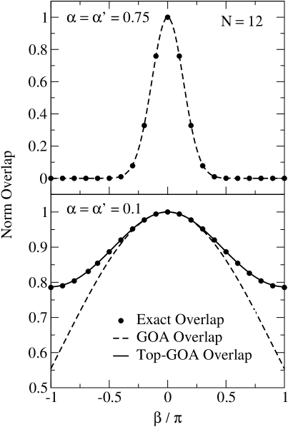
Figure 1: The norm overlaps along $\beta$ direction for two different deformations $\alpha$ as indicated, for the three-level model with $N=12$. The dots show the exact overlaps, dashed lines stand for the standard GOA and full line for topGOA. The topGOA is not shown in the upper panel because it graphically identical with standard GOA.

The effect of GOA versus topGOA for the norm overlap is demonstrated in figure 1. For large deformations (upper panel), the norm overlap decays rather quickly in angle $\beta$. The conventional GOA is here a reliable approximation. The situation is much different at small deformation. The overlaps become broad and hit the periodicity limits. This yields a dramatic difference between GOA and topGOA. Note that topGOA is still an excellent approximation to the exact overlap while GOA fails badly.

III.4 Performance of topGOA

The conventional GOA (9a) maps the Griffin-Hill-Wheeler equation (5) into a collective Schrödinger equation of second order order in the collective momentum GCM ; heenenGCM . This feature is lost in topGOA. Further approximation steps would be needed to come to that end. We will not pursue them further here and solve directly the Griffin-Hill-Wheeler equation (5) inserting the topGOA overlaps (17).

Figure 2: Comparison of energies for the three-level model at various level of approximations as indicated Upper block: Total energies for $N$=12. Lower block: The correlation energy $\Delta E=E-E_{\rm HF}$ for various N as indicated. Results are drawn for a large range of coupling strengths $\chi$ from sphericity $\chi=0$ deeply into the deformed regime.

Figure 2 compares the RPA and topGOA with HF and the exact result for a large variety of coupling strengths. The uppermost panel shows total energies. One sees that both approaches correct the HF energy very far towards the exact energy. However the RPA shows irregularities near the critical point $\chi\approx 1$.

A more detailed look is given in the three lower panels of figure 2 where we show the correlation energies $\Delta E=E-E_{\rm HF}$ for the various approaches and for a series of system sizes. The RPA provides a useful correction in the limits of sphericity and well developed deformations, but fails badly around the critical point. The topGOA performs very well in all regimes. The results improve with increasing system size as one could expect from the Gaussian limit theorem inherent in topGOA. Acceptable results are obtained from topGOA also for $N$=4. But all approaches become inaccurate for $N$=2 which is obviously not collective enough.

III.5 Angular momentum projection

When the mean-field ground state breaks a symmetry of the Hamiltonian, one can get an improved wave function and energy by projection, i.e. take a minimal set of states $q$ and appropriate $f$ in eq. (4) to enforce the symmetry. This is particularly useful for deformations and projection of the $J=0$ ground state ground state out of a deformed intrinsic state. The questions before us are, how does this technique compare with the RPA or the topGOA for computing the correlation energy? It should be noted that the projection method has a formal advantage in that the calculated energy is an upper bound of the true energy associated with the Hamiltonian.

III.5.1 The projected state

We will examine how well the projection technique works for the three-level model as test case. Rotational projection on the ground state angular momentum $M=0$ reads simply

$$|\alpha\rangle_{\rm proj}\propto\int_{-\pi}^{\pi}d\beta\,|\alpha\beta\rangle\quad.$$ (19)

The rotationally projected energy is computed as expectation value which amounts to integrating the overlaps over the angular coordinate $\beta$, i.e.

$$E_{\rm proj}(\alpha)=\frac{\int d(\beta-\beta^{\prime}){\cal H}(\alpha\beta,\alpha\beta^{\prime})}{\int d(\beta-\beta^{\prime}){\cal I}(\alpha\beta,\alpha\beta^{\prime})}\quad.$$ (20)

This is simple and straightforward for the topGOA overlaps of the form (17). We thus can skip the details.

III.5.2 Variation before and after projection

The energy (20) can be computed for any given deformation $\alpha$. The HF ground state deformation $\alpha_{\rm HF}$ is obtained from minimizing the mere HF energy (17e). Applying the projection on this state corresponds to the scheme “variation-before-projection”. It serves to correct for the angular momentum fluctuations in the deformed HF ground state. A much better approach is obtained when performing “variation-after-projection” ring . Here one minimizes the projected energy (20). This is an involved task for exact projection. The topGOA approach yields a simple expression for the projected energy on which a variation is still feasible. It is, of course, particularly simple in the present test case. We just have to search for the deformation $\alpha_{\rm proj}$ which minimizes $E_{\rm proj}$.

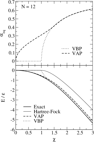
Figure 3: Comparison of variation-after-projection (VAP) and variation-before-projection (VBP) in the three-level model with $N$=12 using exact projection. Upper panel: Ground state deformation $\alpha_{\rm eq}$. Lower panel: Ground state energies from HF and from rotational projection both ways, compared with the exact energy.

Variation-before-projection and variation-after-projection are compared in figure 3 for a large range of coupling strengths. The upper panel shows the ground state deformations. The variation-before-projection state stays spherical up the critical point and switches to deformation with a discontinuous derivate (second order transition). The variation-after-projection states develop more smoothly and show a steady growth of deformation. variation-after-projection can afford intrinsic deformations because it “knows” that projection will restore spherical symmetry. The freedom which variation-after-projection exploits will yield a lower energy. This is shown in the lower panel of figure 3. It is obvious that variation-after-projection picks up a large fraction of the correlation energy at any coupling strength $\chi$, 80% for strongly deformed systems and even more for weakly deformed ones. This makes it obvious that variation-after-projection is the superior strategy. Mind that topGOA helps to simplify variation-after-projection considerably. We will test it now in the next paragraph.

III.5.3 Performance of topGOA for a.m. projection

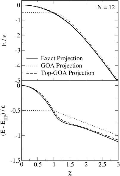
Figure 4: The correlation energy $\Delta E=E_{\rm HF}$ at various levels of approximation for the three-level model N=12. The compared cases are: full = exact projection energy, dotted = projection using standard GOA, dashed = projected energy using topGOA. The upper panel shows the energies as such and the lower panel shows the correlation energy, i.e. the difference to the mere HF energy.

The performance of topGOA for rotational projection is checked in figure 4 for the case of $N$=12. Conventional GOA has obviously problems at small deformation up to beyond the critical point. But topGOA provides a very good approximation to exact projection throughout. And it does that on the grounds of a simple expression for the projected energy which can be deduced from second order moments only. This is welcome for an efficient variation-after-projection and it is particularly helpful in connection with effective energy functionals because double (anti-)commutators with $\hat{H}$ can still be safely derived from second functional derivatives, see Sec. IV E.

The rotational projection can still be done with second order information around the minimum point. It is thus as simple to compute as RPA. And this simple part provides the dominant portion of the correlation energy. The most costly part of the correlation energy is computing the small final contribution from vibrations. It is tempting to consider mere angular projection as a first guess for the correlation energy. That is, in fact, a strategy pursued in the large scale fits of goriely . Our result here provides a welcome substantiation of their “rule of thumb”.

III.6 A thoroughly second order approach: topRPA

The conclusions from the previous subsection encourage the quest for a more efficient estimator of the vibrational correlation energy. And the typical pattern of variation-after-projection add reasons to that. We have seen in figure 3 that the variation-after-projection ground state is nearly always deformed. The projected energy as function of $\alpha$ has always a fairly well developed minimum much in contrast to the HF energy which is rather soft around the critical point. This hints that one is allowed to perform a small amplitude expansion about the projected minimum $\alpha_{\rm proj}$. Once having accepted this idea, the remaining steps are obvious and simple:

1. One performs variation-after-projection using topGOA for rotational projection. This yields the variation-after-projection ground state deformation $\alpha_{0}$.

2. One computes the topGOA projected energy

   $$E_{\rm proj}(\bar{\alpha})=E_{\rm proj}({\alpha}_{0})+\frac{1}{2}(\bar{\alpha}-\alpha_{0})^{2}\partial_{\bar{\alpha}}^{2}E_{\rm proj}(\alpha_{0})$$ (21)

   in the vicinity of $\alpha_{0}$ and deduces the curvature $\partial_{\bar{\alpha}}^{2}E_{\rm proj}$ of this effective potential.

3. For the remaining vibrational correction, one applies the simple correlation energy from harmonic approximation

   $$\delta E_{\rm vib} = \frac{1}{2}\sqrt{\partial_{\bar{\alpha}}^{2}E_{\rm proj}{\cal B}}-\left(\frac{\partial_{\bar{\alpha}}^{2}E_{\rm proj}}{4\lambda_{\rm proj}}+\frac{\lambda_{\rm proj}{\cal B}}{4}\right)\quad,$$ (22a)

   $${\cal B} = \frac{2{\cal H}_{2}^{\alpha}(\alpha_{0})}{\lambda_{\rm proj}^{2}}\quad.$$ (22b)

   $$\lambda_{\rm proj} = 2\partial_{\alpha}\partial_{\alpha^{\prime}}\langle\alpha^{\prime}|\alpha\rangle_{\rm proj}\Big{|}_{\alpha=\alpha^{\prime}=\alpha_{0}},$$ (22c)

   $${\cal H}^{\alpha}_{2}(\alpha_{0}) = \left.2\partial_{\alpha}\partial_{\alpha^{\prime}}\frac{\langle\alpha^{\prime}|\hat{H}|\alpha\rangle_{\rm proj}}{\langle\alpha^{\prime}|\alpha\rangle_{\rm proj}}\right|_{\alpha=\alpha^{\prime}=\alpha_{0}}.$$ (22d)

4. The total energy is then finally

   $$E=\delta E_{\rm proj}(\alpha_{0})-\delta E_{\rm vib}\quad.$$

Note that this scheme requires only information on second order derivatives in $\alpha$ and $\beta$ about the deformed ground state. In that sense it is much similar to RPA. We thus call that scheme topologically corrected RPA (topRPA). The essence is, of course, that topological constraints are exploited to construct from the given second order information the final ground state energy in topRPA.

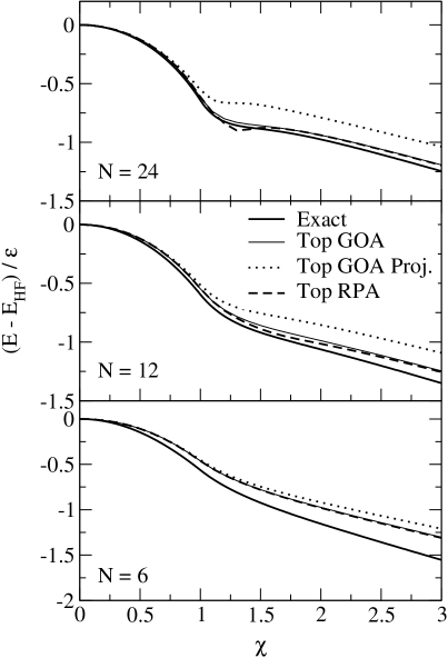
Figure 5: Comparison of topGOA and topRPA for the three-level model and various N as indicated. Upper block: total energies compared with HF and the exact result. Lower block: The correlation energies $E_{\rm scheme}-E_{\rm HF}$ for various levels of approximation. “scheme” stands for the exact solution (full line), the topGOA (dotted line), the topRPA (dashed line). Results are drawn versus effective coupling strength $\chi$.

Figure 5 compares the performance of topRPA and topGOA for the correlation energy in the three-level model. It is obvious that topRPA provides a good approximation to topGOA, equally good for all system sizes. Both schemes constitute a reliable approach to the exact result, better for larger systems. For completeness, we show also the correlation from angular momentum projection alone. We see again that this exhausts the leading part of correlations and could be considered as quick and simple approach. However, topRPA is not much more expensive and comes close to the final result.

IV Particle-Number-Projection

The second test cases in this paper is concerned with particle-number projection. It becomes necessary when starting Hartree-Fock-Bogoliubov (HFB) states, or its BCS approximation, are involved. The HFB approximation produces independent quasi-particle states which have mixed particle number $N$. One needs to project the HFB states onto good particle number. This is important in any nuclear structure calculation because doubly magic nuclei (where mere HF suffices) are an extremely rare species. Similar as in the previous example of rotations-vibrations there is, in principle, a pair of modes, namely particle number projection and pairing vibrations. We confine here the discussion to projection alone because that is the widely used strategy and because it will again exhaust the dominant part of the correlations.

IV.1 Exact projection

Let $|\Phi_{0}\rangle$ be a HFB state with average particle number

$$\langle\Phi_{0}|\hat{N}|\Phi_{0}\rangle=N_{0}\quad.$$ (23)

The projected state with exact particle number $N_{0}$ is

$$|\Psi\rangle\propto\int_{0}^{2\pi}d\eta\,|\eta\rangle\quad,\quad|\eta\rangle=e^{i\eta\tilde{N}}|\Phi_{0}\rangle$$ (24a)

where

$$\tilde{N}=\hat{N}-N_{0}\quad.$$ (24b)

The construction of the path from straightforward $\exp{(i\eta\tilde{N})}$ makes the norm overlap a function of the difference alone, i.e. ${\cal I}={\cal I}(\eta-\eta^{\prime})$. The number conservation $[\hat{H},\tilde{N}]=0$ causes also ${\cal H}={\cal H}(\eta-\eta^{\prime})$. The projected energy thus becomes

$$E=\frac{\int d\eta\langle\Phi_{0}|\hat{H}e^{i\eta\tilde{N}}|\Phi_{0}\rangle}{\int d\eta\langle\Phi_{0}|e^{i\eta\tilde{N}}|\Phi_{0}\rangle}=\frac{\int d\eta\,{\cal H}(\eta)}{\int d\eta\,{\cal I}(\eta)}\quad.$$ (25)

IV.2 The topGOA for particle number projection

IV.2.1 Overlaps and correlation energy

The collective path is $|\eta\rangle$ as given in eq. (24a). The collective coordinate is defined in the interval $[0,2\pi)$ and is periodic as $\eta\longrightarrow\eta+2\pi$. This periodicity is not reproduced by the standard GOA overlaps (9a). One has to modify GOA to account for that structure, in other words one has to employ topologically correct GOA (topGOA). Taking up the experience from the previous test case, we can postulate that the periodic structure of the coordinates is properly taken into account by the argument in GOA through

$$\frac{\eta}{2}\longrightarrow\sin\left(\frac{\eta}{2}\right)\quad.$$

One may wonder why we use this particular assignment for the for the generalization. The choice is unique in that it corresponds to the base period of the squared sine function. Other fractions would not have the correct periodicity of the Hamiltonian. The generalized overlaps for particle-number projection are then

$${\cal I}(\eta) = \exp({-2\langle\tilde{N}^{2}\rangle\sin^{2}\left(\frac{\eta}{2}\right)})\quad,$$ (26a)

$${\cal H}(\eta) = {\cal I}(\eta)\left[{\cal H}_{0}-\frac{1}{2}\sin^{2}\left(\frac{\eta}{2}\right){\cal H}_{2}\right]\quad,$$ (26b)

$${\cal H}_{0} = \langle\Phi_{0}|\hat{H}|\Phi_{0}\rangle=E_{\rm BCS}\quad,$$ (26c)

$${\cal H}_{2} = \langle\{\tilde{N},\{\hat{H}-\langle\hat{H}\rangle,\tilde{N}\}\}\rangle\quad.$$ (26d)

Note that the width $\lambda=2\langle\tilde{N}^{2}\rangle$ and the coefficients ${\cal H}_{i}$ of the Hamiltonian overlap are still defined as in standards GOA, see eq. (9a). What changes is the way how these overlaps are extrapolated. It is obvious that the conventional GOA is recovered in case of steeply decaying norm overlap, i.e. for $\lambda\longrightarrow\infty$.

The projected energy (25) can then be expressed in rather compact fashion as

$$E = E_{\rm BCS}-\delta E_{\rm PNP}\quad,$$ (27a)

$$\delta E_{\rm PNP} = \frac{1}{4}\Lambda\left(\langle\tilde{N}^{2}\rangle\right){\cal H}_{2}\quad,$$ (27b)

$$\Lambda\left(y\right) = \frac{\int_{0}^{2\pi}d\eta\,e^{-2y\sin^{2}\left(\frac{\eta}{2}\right)}2\sin^{2}\left(\frac{\eta}{2}\right)}{\int_{0}^{2\pi}d\eta\,e^{-2y\sin^{2}\left(\frac{\eta}{2}\right)}}\quad.$$ (27c)

The limiting case standard GOA is recovered by

$$\Lambda\longrightarrow 1/(2\langle\tilde{N}^{2}\rangle)\quad\mbox{for}\quad\langle\tilde{N}^{2}\rangle\rightarrow\infty\quad.$$

This corresponds to a HFB state deep in the pairing regime where one gathers substantial particle number fluctuations. The opposite limit is

$$\Lambda\longrightarrow 1\quad\mbox{for}\quad\langle\tilde{N}^{2}\rangle\rightarrow 0\quad.$$

It corresponds to the break down of pairing towards a pure HF state. Standard GOA fails here. It is obvious that only topGOA can cope properly with that pairing transition.

As in case of angular momentum projection, there is the choice between variation-before-projection and variation-after-projection, see section III.5.2. And again variation-after-projection is the preferred method. Variation means here in general variation with respect to the single particle wave functions in the HFB state and its occupation amplitudes $u$ and $v$. The wave functions are fixed in the model which we use later on and only the variation of $u$ and $v$ remains to be done.

IV.3 RPA correlations

The correlation energy in RPA is computed with eq. (1). The mode corresponding to particle-number phase is given by the path (24a). It is found as zero-energy mode in the RPA spectrum because of $[\hat{H},\hat{N}]=0$. Thus one knows already the combination $\hat{N}\equiv\hat{Q}=\left(\hat{C}^{+}+\hat{C}\right)/\sqrt{2}$. The conjugate combination (3) has to be determined by linear response $[\hat{H},\hat{P}_{N}]\propto\hat{N}$. Once having the pair $(\hat{N},\hat{P}_{N})$, one can easily compute the correlation energy (1).

IV.4 A simple model as test case

IV.4.1 The model

For further testing of the approximate scheme, we need a schematic model. It should have a gap in the single-particle spectrum to model the interplay between this gap and the pairing strength. Thus we take a two-shell model with lower band $s=-1$ and upper band $s=+1$. Each band is $N$-fold degenerated as $m=-(N-1)/2,\cdots,+(N-1)/2$. The states $\pm m$ are considered as the pairing conjugate partners. This yields the generalized Lipkin-Meshkov-Glick model introduced in Ref. feldman . It is simply a two-level model with seniority pairing. The model Hamiltonian reads

$$\hat{H} = \epsilon\sum_{sm}s\,\alpha_{sm}^{+}\alpha_{sm}^{\mbox{}}$$ (28)

$$-\chi\frac{2\epsilon}{N}\left(\sum_{s,m\!>\!0}\alpha_{sm}^{+}\alpha_{s-m}^{+}\right)\left(\sum_{s,m\!>\!0}\alpha_{s-m}^{\mbox{}}\alpha_{sm}^{\mbox{}}\right)\quad.$$

We associate the following single-particle energies and occupation amplitudes

$$\begin{array}[]{ll}\varepsilon_{1}=\varepsilon&v_{1}=u_{-1}=u=\sqrt{1-v^{2}}\\ \varepsilon_{-1}=-\varepsilon&v_{-1}=u_{1}=v\end{array}$$ (29)

Note that the Fermi energy is $\varepsilon_{F}=0$ for symmetry reasons.

The exact solution can be obtained by diagonalizing the Hamiltonian (28) using the quasi-spin formalism, for details see HB00 .

IV.4.2 The energy in topGOA

The model is sufficiently simple that everything can be worked out analytically. The final result projected energy in topGOA becomes

$$\frac{E_{\rm BCS}}{N\varepsilon} = -\left(\sqrt{1-(2uv)^{2}}+\frac{\chi}{2}(2uv)^{2}\right)\quad,$$ (30a)

$$\delta E_{\rm PNP} = E_{\rm BCS}\left[1+(2uv)^{2}\Lambda\left(\frac{N}{2}(2uv)^{2}\right)\right]\quad.$$ (30b)

This energy needs now to be compared with the BCS approximation $E_{\rm BCS}$, the RPA energy, and the exact energy.

IV.4.3 The energy in RPA

As shown in HB00 , there are two collective modes in this model. For small values of $\chi$, the mean field approximation does not support the BCS solution and only the trivial solution with zero pairing gap $\Delta=0$ appears. In this regime, the two RPA frequencies are similar to each other, see Ref. HB00 for the explicit expressions. At $\chi\sim N/(N-1)$, the system undergoes phase transition to the superfluid phase, and the number fluctuating BCS solution becomes the ground state in the mean field approximation. Consequently, one of the RPA frequencies becomes zero due to the number conservation of the Hamiltonian (28). Applying eq.(1) with the symmetry mode yields the the RPA correlation energy

$$\Delta E_{\rm RPA}=-\frac{\epsilon\chi}{2}.$$ (31)

The RPA frequency of the other mode is given by 2$\Delta=4\epsilon\chi(uv)$. This mode corresponds to the pairing vibration whose contribution is omitted here because we study just the projection part.

Figure 6: Upper panel: total energies at various levels of approximation for a system with $N=12$ particles obeying the Hamiltonian (28). Lower three panels: The correlation energy $\Delta E=E_{\rm BCS}$ for systems with different $N$ as indicated.

IV.4.4 A few words on the Lipkin-Nogami approach

Full projection is often difficult, the more so if used in connection with variation-after-projection. Thus one often employs approximate schemes for particle-number projection.

A widely used approximation scheme for particle-number projection is the Lipkin-Nogami approach, see e.g. Pra73a and references cited therein. It provides a good numerical approximation of the variation-after-projection in situations where both the HFB equations predict a collapse of the pairing correlations. The prescription of Lipkin-Nogami amounts to modify the energy by adding the second-order Kamlah correction $\lambda_{2}(\hat{N}-\langle\hat{N}\rangle)^{2}$ where $\lambda_{2}$ is computed from mixed variances of $\hat{N}$ and $\hat{H}$, see e.g. for Skyrme-Hartree-Fock Rei96 . The modification of the HFB equations associated with the Lipkin-Nogami prescription is obtained by a restricted variation of where $\lambda_{2}$ is not varied although its value is calculated from self-consistent expectation values. For a thorough discussion of the approximations involved see Flo97a ; DN93 . Note that the Kamlah expansion, and therefore the Lipkin-Nogami approach, uses the similar expansion as the naive GOA and does not take into account the topology of the gauge angle $\eta$.

IV.5 Results and discussion

The upper part of figure 6 shows the total energy in the two-level model with seniority pairing for $N$=12 particles. Various approximations are considered. The BCS is the uncorrelated result. It decreases with constant slope up to $\chi\approx 1.1$ which is the transition point from pure HF (for smaller $\chi$) to a truly pairing HFB state (for larger $\chi$). The exact energy is the goal. In addition to RPA and topGOA, we show also the results from the Lipkin-Nogami scheme (see section IV.4.4). It is obvious from the figure that all corrections improve the BCS energy towards the exact result. The RPA correction works fine except for the region around the critical point. That is understandable because the critical point is distinguished by large fluctuations and RPA is designed to be a theory for small amplitude. The Lipkin-Nogami result has a smoother trend than RPA and correct the energy in the wanted direction. However the correction is incomplete, particularly at small coupling $\chi$ HB00 . Last but not least, the topGOA provides a very good approximation throughout all coupling strengths. It is clearly superior to the competing projection approach, the Lipkin-Nogami scheme, and it is more robust than RPA around the transition point.

A more detailed comparison of the various approaches is shown in the lower panels of figure 6. It displays the correlation energies which point out the differences more clearly. First of all, the correlation energy stays about independent of system size while the total energy grows $\propto N$. This means that the relative importance of correlations shrinks as $1/N$. This corroborates the known effect that mean field models, here represented by BCS, become exact in the limit $N\longrightarrow\infty$. The Lipkin-Nogami scheme maintains its feature to produce a “half-way” correction. It is a little bit surprising that the mismatch becomes even more pronounced with increasing system size. The RPA, on the other hand, clearly improves for larger systems. That is not surprising because mean field theories are restored in the large $N$ limit, and RPA is a theory of vibrating mean fields. Finally, the topGOA provides a reliable and robust approximation to the exact correlation energy at all system sizes and coupling strengths. There are regions where it is near to perfect. There are regions where one obtains visible deviations of a few percent. But the trends are always smooth and the average performance is excellent.

There are two more particularly appealing aspect of particle-number projection with topGOA:

1. The project energy (27) is a closed expression in terms of expectation values of $\hat{H}$ in combination with $\hat{N}$ and of the occupation amplitudes $u$ and $v$. One can easily use that as starting point for “variation after projection”. Variation with respect to the single particle wave functions yields the appropriate correction terms to the mean field equations. These terms can easily be incorporated in existing codes.

2. The full GCM is not applicable in connection with nuclear density functionals, as e.g. the Skyrme-Hartree-Fock energy. The energy-density functional is given for an expectation value with one mean field state. The extension to overlaps with different states at $q$ and $q^{\prime}$ is ambiguous. But an extension of the functional is still feasible in the immediate vicinity of a mean field state. Thus the second order expression ${\cal H}_{2}$ in (26d) can still be derived within the safe grounds of density-functional theory. The topGOA thus provides a means to compute particle number projection safely for Skyrme-Hartree-Fock.

V Conclusions

We have investigated the efficient computation of ground state correlations for low-energy modes and projection. Starting point is the generator coordinate method (GCM). It is considered in the Gaussian overlap approximation (GOA) which reduces the formal and numerical expense dramatically because it involves only expectation values and second order variations therefrom. We have shown that GOA runs into troubles in cases of weak coupling (thus broad overlaps) for coordinates with non-trivial topology. A slight modification of the scheme allows to tune a topologically correct GOA (topGOA). We have demonstrated and tested topGOA for two typical cases of collective coordinates, rotation-vibration and particle-number projection. To that end, we employed exactly solvable models in the spirit of the Lipkin-Meskov-Glick model.

The straightforward cases are mere projection (test cases: angular momentum and particle number). It was found that topGOA provides an excellent approximation to full projection. Performing variation after projection (variation-after-projection) allows to incorporate already a great deal of correlations into the projected states. The topGOA is particularly well suited for variation-after-projection because the projected energy is expressed in simple and compact expressions on which one can perform variation with moderate expense, far simpler than for exact projection (where non-orthogonal overlaps complicate matters). In particular for particle number projection, topGOA thus offers a simple and in all regimes reliable scheme which allows a thoroughly variational formulation. It is superior to the Lipkin-Nogami scheme in that respect.

Mere angular momentum projection with variation-after-projection was shown to grab a large portion of the correlation energy. Yet it is incomplete without the vibrational part. We have tested topGOA for the coupled rotations-vibrations and it performs well in all regimes, near sphericity, at the transition point, and for well deformed nuclei. As one could expect for a Gaussian limit, the performance improves with system size. The reverse is also true: small systems are more critical and a two-particle system is off limits.

The topGOA for vibrations involves, in principle, large amplitude motion. This can become inconvenient in practice because a whole collective deformation path has to be mapped. The better defined deformation of the variation-after-projection ground state allowed a small amplitude expansion of topGOA. The result is a scheme which can live with second order expression around the projected ground state. We consider it as a topological generalization of the random-phase approximation (RPA) which also deals with second order expressions throughout and call this new scheme topological RPA (topRPA). We find that topRPA provides a good approximation to the results of topGOA and thus to the exact correlation energy for rotations-vibrations.

Altogether, we have developed with the help of topologically corrected Gaussian overlaps a palette of useful approximations for computing very efficiently collective correlations on top of nuclear mean-field calculations. The next step is to implement that into practical calculations. Work in that direction is in progress.

References

- (1) P.-G. Reinhard, C. Toepffer, Int.J.Mod.Phys. E 3 (1994) 435.
- (2) D.J. Rowe, Nuclear Collective Motion, Methuen, London, 1970.
- (3) G.F. Bertsch and R.A. Broglia, Oscillations in finite quantum systems, Cambridge University Press, Cambridge, 1994.
- (4) P.-G. Reinhard, K. Goeke, Rep.Prog.Phys. 50 (1987) 1
- (5) P. Bonche, J. Dobaczewski, H. Flocard, P.H. Heenen, J. Meyer, Nucl.Phys. A510 (1990) 466
- (6) K.W. Schmid, P.-G. Reinhard, Nucl.Phys. A 530 (1991) 283
- (7) M. Samyn, S. Goriely, P.–H. Heenen, J. M. Pearson, F. Tondeur, Nucl. Phys. A, in press
- (8) H.C. Pradhan, Y. Nogami, J. Law, Nucl.Phys. A 201 (1973) 357
- (9) P.-G. Reinhard, Z.Phys. A 285 (1978) 93
- (10) A. Gozdz, K. Pomorski, M. Brack, W. Werner, Nucl.Phys. A 442 (1985) 50
- (11) H.J. Lipkin, N. Mechkov, and A.J. Glick, Nucl. Phys. 62 (1965) 188; ibid.62 (1965) 199; ibid.62 (1965) 211.
- (12) P. Ring, P. Schuck, The Nuclear Many-Body Problem, Springer, Berlin 1989
- (13) N. Fukuda, F. Iwamoto, and K. Sawada, Phys. Rev. 135 (1964) A932.
-
(14)
D.J. Rowe, Phys.Rev. 175 (1968) 1283;
J.C. Parikh, D.J. Rowe, Phys.Rev. 175 (1968) 1293 - (15) K. Hagino, G. Bertsch, Phys.Rev. C 61 (2000) 024307
- (16) B. Jancovici and D.H. Schiff, Nucl.Phys. 58 (1964) 678.
- (17) D.M. Brink and A. Weiguny, Nucl. Phys. A120 (1968) 59.
- (18) J.L. Egido, L.M. Robledo, Nucl.Phys. A 494 (1989) 85
- (19) P.H. Heenen, A. Valor, M. Bender, P. Bonche, and H. Flocard, Eur. Phys. J. A11 (2001) 393.
- (20) P.–G. Reinhard, W. Nazarewicz, M. Bender, J. A. Maruhn, Phys.Rev. C 53 (1996) 2776
- (21) H. Flocard, N. Onishi, Ann.Phys. (NY) 254 (1997) 275
- (22) J. Högaasen-Feldman, Nucl. Phys. 28 (1961) 258.
- (23) K. Hagino and G.F. Bertsch, Nucl. Phys. A 679 (2000) 163.
- (24) J. Dobaczewski and W. Nazarewicz, Phys. Rev. C47 (1993) 2418.