MKPH-T-02-01
The $\eta$-$3N$ problem with separable interactions

Abstract

The $\eta$-$3N$-interaction is studied within the four-body scattering theory adopting purely separable forms for the two- and three-body subamplitudes, limiting the basic two-body interactions to $s$-waves only. The corresponding separable approximation for the integral kernels is obtained by using the Hilbert-Schmidt procedure. Results are presented for the $\eta$-³H scattering amplitude and for the total elastic cross section for energies below the triton break-up threshold.

PACS numbers: 13.60.Le, 21.45.+v, 25.20.Lj

I Introduction

In the last ten years the interaction of $\eta$-mesons with few-nucleon systems has attracted considerable interest, and quite a large amount of research has been carried out both on the experimental as well as on the theoretical side. The major aim of this activity is to obtain a well-defined conceptual picture of the low-energy $\eta$-nuclear interaction which then may serve to clarify the foundation of the more fundamental $\eta N$ problem.

Of special interest is the $\eta$-$3N$-system, for which exactly soluble models are available. At the same time it encloses a much wider range of phenomena than the more simple $\eta NN$ case. In this context we would also like to mention several precise experimental investigations of $\eta$-production on three-body nuclei performed during the last decade [1, 2, 3]. Previous theoretical studies in this area were restricted to various approximations in treating the few-particle aspects of this problem. As an earlier nonperturbative calculation, we would like to refer to the optical model approach of [4], whose purpose was to estimate qualitatively the possible formation of bound $\eta$-meson states with the lightest nuclei. More refined calculations were presented in [5], where the authors were able to sum the multiple scattering series for the $\eta$-³H amplitude, including several important corrections to the trivial optical limit. Another result reported in [6] were obtained within the so-called finite-rank-approximation (FRA) which has recently been applied also to the $\eta$-production from three-body nuclei [7, 8]. The crucial point of this model is the neglect of target excitations during the interaction with the $\eta$-meson. Clearly this assumption allows one to avoid the complications associated with the direct solution of the four-body dynamical equations. Concerning the present study, we were guided by the idea that the approximations used in many-body physics, such as the optical model or adiabatic treatment of the target, may fail when few-particle systems are studied. Especially, this seems to be true for small kinetic energies, where the unitarity conditions of the scattering matrix, nucleon recoil and other effects become significant. Their neglect, tolerated in various many-body approaches, may affect drastically the quality of the few-body results. Therefore, the present work is intended to solve the $\eta$-$3N$-problem without making any such not well controlled approximations.

The basis of our calculation is the four-body formalism in momentum space. Although a variety of methods for solving the n-particle problem has been proposed in the literature, the Faddeev-Yakubovsky theory [9, 10] and the one of Alt, Grassberger and Sandhas (AGS) [11, 12] are most convenient and preferred for practical applications. Adopting the separable representation for the driving two-body potentials as well as for the subamplitudes appearing in the (1+3)- and (2+2)-partitions of the four-body system, both approaches lead to the same set of effective two-body equations [11, 13, 14]. As is well known, the separable approximation of the integral kernels permits one to represent the dynamical equations in terms of particle exchange diagrams. Due to this tractability and its relatively simple numerical realization, this method has received wide acceptance in few-body physics. Thus at present, a feasible formalism of four-particle theory has been extensively developed, despite the much more complex structure of the corresponding equations compared to the three-body case. After the work of Tjon [15] impressive results have been obtained in recent years for the four-nucleon low-energy interaction (see e.g. [16] and references therein), as well as for pion absorption on three-nucleon systems [19, 20, 21]. With respect to other techniques we would like to refer to recent work in [17] and [18].

The paper is organized as follows. In the next section we outline briefly the formal aspects concerning the application of the four-body formalism to the $\eta$-$3N$ system within the quasiparticle approach. Besides the basic equations we introduce here the two- and three-body ingredients of the model. Our results for $\eta$-³H elastic scattering are presented in Sect. III, and conclusions are drawn in the last section. Details are given in two appendices.

II Application of the four-body formalism to the $\eta$-$3N$ system

The separable method is well known to allow one to reduce the $n$-body problem to an in general simpler $(n-1)$-body case, where one of the constituents appears as a quasiparticle, i.e., a two-body bound, virtual or resonance state. In particular, the three-body equations for the (3$\to$3) transition amplitudes are exactly reduced to effective two-particle equations of Lippmann-Schwinger type. Their kernels contain the off-energy-shell (2$\to$2) amplitudes for all two-body subsystems. In an analogous manner, the four-body scattering kernels can be expressed in terms of subamplitudes stemming from the decomposition of the four-body system into the partitions (1+3) and (2+2). Therefore, approximating these subamplitudes once more by a separable ansatz we can again reduce the four-body problem to an effective quasiparticle two-body one. The formal details of this two-step reduction scheme may be found in Refs. [11, 13, 14]. Here we restrict ourselves to a brief description of the resulting quasi-two-body equations as applied to the $\eta$-$3N$ system.

A The four-body $\eta$-$3N$ equations

Since our formalism does not include Coulomb forces, we will consider for definiteness the $\eta$-³H interaction throughout this paper. All appropriate states are assumed to be properly antisymmetrized with respect to the nucleons. The corresponding antisymmetrization procedure is outlined in Appendix A. Then we are led to the following three channels, corresponding to three possible two-quasiparticle partitions of the $\eta$-$3N$ system

$$(1)\!:\ \eta+(3N)\,,\quad(2)\!:\ N+(\eta NN)\,,\quad(3)\!:\ (N\eta)+(NN)\,.$$ (1)

We only need the amplitudes connecting the initial asymptotic state, consisting of the $3N$ bound state (³H) and a free $\eta$-meson, with all three channels listed in (1). They obey a set of three coupled integral equations (see Appendix A), whose structure is represented by the following matrix equation

$$\left(\begin{array}[]{c}X_{1}\\ X_{2}\\ X_{3}\end{array}\right)=\left(\begin{array}[]{c}0\\ Z_{21}\\ Z_{31}\end{array}\right)+\left(\begin{array}[]{ccc}0&Z_{12}&Z_{13}\\ Z_{21}&Z_{22}&Z_{23}\\ Z_{31}&Z_{32}&0\\ \end{array}\right)\left(\begin{array}[]{cccc}\Theta_{1}&&\\ &\Theta_{2}&\\ &&\Theta_{3}\end{array}\right)\left(\begin{array}[]{c}X_{1}\\ X_{2}\\ X_{3}\end{array}\right)\,.$$ (2)

Here the index $\alpha$=1, 2, 3 stands for the channel $(\alpha)$ from (1). The amplitude $X_{\alpha}$ describes the transition $(1)\to(\alpha)$. The effective potentials $Z_{\alpha\beta}$ are expressed in terms of the form factors, generated by the separable representation of the subamplitudes appearing in the channels (1).

Because here we consider only low energy scattering, we take into account only the dominant $s$-wave part of the interaction in the two-body subsystems and thus only $s$-waves in the three- and four-particle states. Therefore, the matrix elements are diagonal with respect to the total spin $S$. For the elastic $\eta$-³H scattering we need to consider only those states where the spins and isospins of all nucleons are coupled to $S=T=1/2$. In all expressions to follow we drop the index $L=0$. The explicit analytical form of the potentials $Z_{\alpha\beta}$, taking into account the spin-isospin degrees of freedom, is given in the Appendix B. In a more detailed notation the system (2) reads

$$X_{\alpha;nn^{\prime}}^{(ss^{\prime})}(p,p^{\prime},E) = (1-\delta_{\alpha 1})Z_{\alpha 1;nn^{\prime}}^{(ss^{\prime})}(p,p^{\prime},E)$$ (4)

$$+\sum_{\beta=1}^{3}\Big{(}1-\delta_{\alpha\beta}(1-\delta_{\alpha 2})\Big{)}\sum\limits_{n^{\prime\prime}s^{\prime\prime}}\int\limits_{0}^{\infty}Z_{\alpha\beta;nn^{\prime\prime}}^{(ss^{\prime\prime})}(p,p^{\prime\prime},E)\Theta_{\beta;n^{\prime\prime}}({\cal E}_{\beta})X_{\beta;n^{\prime\prime}n^{\prime}}^{(s^{\prime\prime}s^{\prime})}(p^{\prime\prime},p^{\prime},E)\,\frac{p^{\prime\prime 2}\,dp}{2\pi^{2}}\,.$$

The index $s=(0,1)$ in the above equations corresponds to the total spin of the given $NN$ pair. Clearly, due to the pseudoscalar-isoscalar nature of the $\eta$-meson, the value of $s$ fixes uniquely the spin structure of the overall 4-body state with total spin $S$=1/2. In view of the limitation of the two-body interaction to the dominant $s$-wave part, the isospin $t$ of a $NN$ pair is fixed by its spin $s$ through the condition $s+t=1$. The subenergies ${\cal E}_{\beta}$ in (4) are defined as

$${\cal E}_{\beta}=E-\frac{p^{\prime\prime 2}}{2M_{\beta}}\,,\ (\beta=1,2,3)\,,$$ (5)

with reduced masses

$$M_{1}=\frac{3M_{N}m_{\eta}}{3M_{N}+m_{\eta}},\ M_{2}=\frac{M_{N}(2M_{N}+m_{\eta})}{3M_{N}+m_{\eta}},\ M_{3}=\frac{2M_{N}(M_{N}+m_{\eta})}{3M_{N}+m_{\eta}}.$$ (6)

A graphical representation of the system (4) is shown in Figs. 1 and 2.

The structure of (2) allows one to eliminate the channel (1) yielding an equivalent set of only two coupled equations for the amplitudes $X_{2}$ and $X_{3}$. In detail, one has for $\alpha\in\{2,\,3\}$

$$X_{\alpha;nn^{\prime}}^{(ss^{\prime})}(p,p^{\prime},E) = Z_{\alpha 1;nn^{\prime}}^{(ss^{\prime})}(p,p^{\prime},E)+\sum_{\beta=2,3}\sum\limits_{n^{\prime\prime}s^{\prime\prime}}\int\limits_{0}^{\infty}\widetilde{Z}_{\alpha\beta;nn^{\prime\prime}}^{(ss^{\prime\prime})}(p,p^{\prime\prime},E)\Theta_{\beta;n^{\prime\prime}}({\cal E}_{\beta})X_{\beta;n^{\prime\prime}n^{\prime}}^{(s^{\prime\prime}s^{\prime})}(p^{\prime\prime},p^{\prime},E)\,\frac{p^{\prime\prime 2}\,dp}{2\pi^{2}}\,,$$ (7)

where the new effective potentials are given by ($\alpha,\,\beta\in\{2,\,3\}$)

$$\widetilde{Z}_{\alpha\beta;nn^{\prime}}^{(ss^{\prime})}(p,p^{\prime},E) = \Big{(}1-\delta_{\alpha\beta}(1-\delta_{\alpha 2})\Big{)}Z_{\alpha\beta;nn^{\prime}}^{(ss^{\prime})}(p,p^{\prime},E)$$ (9)

$$+\sum\limits_{n^{\prime\prime}s^{\prime\prime}}\int\limits_{0}^{\infty}Z_{\alpha 1;nn^{\prime\prime}}^{(ss^{\prime\prime})}(p,p^{\prime\prime},E)\Theta_{1;n^{\prime\prime}}({\cal E}_{1})Z_{1\beta;n^{\prime\prime}n^{\prime}}^{(s^{\prime\prime}s^{\prime})}(p^{\prime\prime},p^{\prime},E)\frac{p^{\prime\prime 2}dp^{\prime\prime}}{2\pi^{2}}\,.$$

After solving the system (7), the amplitude $X_{1}$ is obtained from

$$X_{1;nn^{\prime}}^{(ss^{\prime})}(p,p^{\prime},E) = \sum_{\beta=2,3}\sum\limits_{n^{\prime\prime}s^{\prime\prime}}\int\limits_{0}^{\infty}Z_{1\beta;nn^{\prime\prime}}^{(ss^{\prime\prime})}(p,p^{\prime\prime},E)\Theta_{\beta;n^{\prime\prime}}({\cal E}_{\beta})X_{\beta;n^{\prime\prime}n^{\prime}}^{(s^{\prime\prime}s^{\prime})}(p^{\prime\prime},p^{\prime},E)\,\frac{p^{\prime\prime 2}dp}{2\pi^{2}}\,.$$ (10)

The set of equations (7) is more suitable for the numerical solution than (4), since in the former case the integration over the triton pole in the propagator $\Theta_{1}$ may be carried out independently from the procedure of solving the system (7) itself. Thus the kernels in (7) are smooth functions of the integration variable, and the equations may be solved by direct matrix inversion. We recall that below the triton break-up threshold we are dealing with only nonsingular potentials $Z_{\alpha\beta}$.

B The subamplitudes

The key ingredient of the quasiparticle method [11, 14], leading to the equations of the type (4), is the separable representation of the off-shell scattering amplitudes for the two- and three-body subsystems, appearing in the (2+2)- and (1+3)-partitions. In our case, the two types of two-body subsystems involved are $NN$ and $\eta N$, denoted in the following by “$d\,$” and “$N^{*}$”, respectively. For the corresponding scattering matrices we adopt the simplest rank-one separable form. In detail, we use for the $NN$ interaction

$$t_{d}^{(s)}(q,q^{\prime},z)=g_{d}^{(s)}(q)\tau_{d}^{(s)}(z)g_{d}^{(s)}(q^{\prime})\,,$$ (11)

with

$$\tau_{d}^{(s)}(z)=-\frac{1}{2M_{N}}\,\Big{[}1-\frac{1}{4\pi^{2}}\int\limits_{0}^{\infty}\frac{[g^{(s)}_{d}(q)]^{2}}{zM_{N}-q^{2}}\,q^{2}dq\Big{]}^{-1}\,.$$ (12)

Here the upper index $(s)$ stands for the singlet $(s=0)$ and triplet $(s=1)$ $NN$ states. For the form factors $g_{d}^{(s)}(q)$ we use the simplest parameterization

$$g_{d}^{(s)}(q)=g_{d}^{(s)}\frac{\beta^{2}_{s}}{\beta^{2}_{s}+q^{2}}\,.$$ (13)

Analogously, we choose in the $\eta N$ channel

$$t_{N^{*}}(q,q^{\prime},z)=g_{N^{*}}^{\eta}(q)\tau_{N^{*}}(z)g_{N^{*}}^{\eta}(q^{\prime})\,,$$ (14)

with

$$\tau_{N^{*}}(z)=-\Big{[}z+M_{N}+m_{\eta}-M_{0}-\Sigma_{\eta}(z)-\Sigma_{\pi}(z)\Big{]}^{-1}\,,$$ (15)

where

$$\Sigma_{\rho}(z)=\int\limits_{0}^{\infty}\frac{[g_{N^{*}}^{\rho}(q)]^{2}}{z+m_{\eta}-m_{\rho}-\frac{q^{2}}{2\mu_{\rho N}}+i\epsilon}\,\frac{q^{2}dq}{2\pi^{2}}\,,$$ (16)

and

$$g_{N^{*}}^{\rho}(q)=g_{N^{*}}^{\rho}\frac{\beta^{2}_{\rho}}{\beta^{2}_{\rho}+q^{2}}\,,\ \ \mu_{\rho N}=\frac{M_{N}m_{\rho}}{M_{N}+m_{\rho}}\,,\ \quad\rho\in\{\pi,\eta\}\,.$$ (17)

The parameters appearing in (13), (15) and (17) are summarized in Table I. Those for the $NN$ interaction were taken from the low-energy $NN$ fit presented in [22], and the $\eta N$-parameters are chosen as to reproduce the scattering length $a_{\eta N}=(0.75+i\,0.27)$ fm which agrees with the most recent results [23, 24]. However, our parameterization gives a different value for the effective range parameter $r_{0}=(1.95+i\,0.07)$ fm compared to $r_{0}=(1.5+i\,0.24)$ fm of [24]. Unfortunately, we are not able to fit both values $a_{\eta N}$ and $r_{0}$ simultaneously, which is of course the price one has to pay for using the simplest separable ansatz (11). When comparing our predictions with those of [5, 6] we use also other sets of $\eta N$-parameters chosen in such a way that they lead in each case to the corresponding value of $a_{\eta N}$ used there (see Table III).

Turning now to the general scheme, we have to introduce also the separable representation for the three-body subamplitudes, which will then serve as a necessary input for the four-body calculation. For this purpose we apply the Hilbert-Schmidt expansion. The main formal aspects of the procedure can be found e.g. in [25, 26].

The three-nucleon $s$-wave doublet amplitudes $U_{1;ss^{\prime}}$, appearing in the channel (1) obey the equation (see e.g. [27])

$$U_{1;ss^{\prime}}(q,q^{\prime},{\cal E})=V_{1;ss^{\prime}}(q,q^{\prime},{\cal E})+\!\sum\limits_{s^{\prime\prime}=0,1}\int\limits_{0}^{\infty}V_{1;ss^{\prime\prime}}(q,q^{\prime\prime},{\cal E})\,\tau_{d}^{(s^{\prime\prime})}\!\Big{(}{\cal E}-\frac{3q^{\prime\prime 2}}{4M_{N}}\Big{)}U_{1;s^{\prime\prime}s^{\prime}}(q^{\prime\prime},q^{\prime},{\cal E})\frac{q^{\prime\prime 2}dq^{\prime\prime}}{2\pi^{2}}\,,\quad s,s^{\prime}=0,1\,.$$ (18)

The effective potentials are defined in terms of the form factors $g_{d}(k)$ of the two-nucleon amplitude (11) as

$$V_{1;ss^{\prime}}(q,q^{\prime},{\cal E})=\frac{\Lambda_{ss^{\prime}}}{2}\int\limits_{-1}^{+1}\frac{g_{d}^{(s)}(|\vec{q}\,^{\prime}+\frac{1}{2}\vec{q}\,|)\ g_{d}^{(s^{\prime})}(|\vec{q}+\frac{1}{2}\vec{q}\,^{\prime}|)}{{\cal E}-\frac{q^{2}}{M_{N}}-\frac{q^{\prime 2}}{M_{N}}-\frac{\vec{q}\cdot\vec{q}\,^{\prime}}{M_{N}}}d(\hat{q}\cdot\hat{q}^{\prime})\,,\ \quad s,s^{\prime}=0,1\,,$$ (19)

where ${\cal E}$ denotes the total c.m. kinetic energy in the three nucleon system, and the matrix of the spin-isospin coefficients is given by

$$\Lambda=\left(\begin{array}[]{rr}\frac{1}{2}&-\frac{3}{2}\\ &\\ -\frac{3}{2}&\frac{1}{2}\end{array}\right)\,.$$ (20)

The Hilbert-Schmidt expansion for the driving term $V_{1;ss^{\prime}}$ reads

$$V_{1;ss^{\prime}}(q,q^{\prime},{\cal E})=-\sum\limits_{n}\lambda_{n}({\cal E})u^{(s)}_{n}(q,{\cal E})u^{(s^{\prime})}_{n}(q^{\prime},{\cal E})\,,$$ (21)

where the functions $u_{n}^{(s)}(q,{\cal E})$ are taken as the eigenfunctions of the kernel of equation (18) with the eigenvalues $\lambda_{n}$, i.e.

$$u^{(s)}_{n}(q,{\cal E})=\frac{1}{\lambda_{n}({\cal E})}\sum\limits_{s^{\prime}=0,1}\int\limits_{0}^{\infty}V_{1;ss^{\prime}}(q,q^{\prime},{\cal E})\,\tau^{(s^{\prime})}_{d}\!\Big{(}{\cal E}-\frac{3q^{\prime 2}}{4M_{N}}\Big{)}u^{(s^{\prime})}_{n}(q^{\prime},{\cal E})\frac{q^{\prime 2}dq^{\prime}}{2\pi^{2}}\,,\ \quad s=0,1\,.$$ (22)

They are normalized according to

$$\sum\limits_{s=0,1}\int\limits_{0}^{\infty}u^{(s)}_{n}(q,{\cal E})\,\tau^{(s)}_{d}\!\Big{(}{\cal E}-\frac{3q^{2}}{4M_{N}}\Big{)}u^{(s)}_{n^{\prime}}(q,{\cal E})\frac{q^{2}dq}{2\pi^{2}}=-\delta_{nn^{\prime}}\,.$$ (23)

The separable form of the amplitude can easily be found

$$U_{1;ss^{\prime}}(q,q^{\prime},{\cal E})=\sum\limits_{n}u^{(s)}_{n}(q,{\cal E})\Theta_{1;n}({\cal E})u^{(s^{\prime})}_{n}(q^{\prime},{\cal E})\,,\ \quad\Theta_{1;n}({\cal E})=\frac{\lambda_{n}({\cal E})}{\lambda_{n}({\cal E})-1}\,.$$ (24)

The amplitudes for the $\eta NN$ scattering, related to the channel (2) and denoted in the following by $\overline{U}_{2;ij}$ with $i,j\in\{d,N^{*}\}$, are coupled into two independent sets corresponding to two possible spin-isospin $\eta NN$ $s$-wave states $(S;T)=(0;1)$ and $(1;0)$, denoted by an upper index $(s)$ with $s\in\{0,1\}$, each of the form

$$\overline{U}^{(s)}_{2;dd}(q,q^{\prime},{\cal E}) = \int\limits_{0}^{\infty}V^{(s)}_{2;dN^{*}}(q,q^{\prime\prime},{\cal E})\,\tau_{N^{*}}\!\Big{(}{\cal E}-\frac{q^{\prime\prime 2}}{2\widetilde{\mu}_{N^{*}}}\Big{)}\overline{U}^{(s)}_{2;N^{*}d}(q^{\prime\prime},q^{\prime},{\cal E})\frac{q^{\prime\prime 2}dq^{\prime\prime}}{2\pi^{2}}\,,$$ (25)

$$\overline{U}^{(s)}_{2;N^{*}d}(q,q^{\prime},{\cal E}) = V^{(s)}_{2;N^{*}d}(q,q^{\prime},{\cal E})+\int\limits_{0}^{\infty}\Big{[}V^{(s)}_{2;N^{*}d}(q,q^{\prime\prime},{\cal E})\,\tau^{(s)}_{d}\!\Big{(}{\cal E}-\frac{q^{\prime\prime 2}}{2\widetilde{\mu}_{d}}\Big{)}\overline{U}^{(s)}_{2;dd}(q^{\prime\prime},q^{\prime},{\cal E})$$ (27)

$$\hskip 56.9055pt+V^{(s)}_{2;N^{*}N^{*}}(q,q^{\prime\prime},{\cal E})\,\tau_{N^{*}}\!\Big{(}{\cal E}-\frac{q^{\prime\prime 2}}{2\widetilde{\mu}_{N^{*}}}\Big{)}\overline{U}^{(s)}_{2;N^{*}d}(q^{\prime\prime},q^{\prime},{\cal E})\Big{]}\frac{q^{\prime\prime 2}dq^{\prime\prime}}{2\pi^{2}}\,.$$

The reduced masses appearing in (25) are defined by

$$\widetilde{\mu}_{N^{*}}=\frac{M_{N}(M_{N}+m_{\eta})}{2M_{N}+m_{\eta}},\ \ \widetilde{\mu}_{d}=\frac{2M_{N}m_{\eta}}{2M_{N}+m_{\eta}}\,.$$ (28)

The corresponding effective potentials are

$$V^{(s)}_{2;dd}(q,q^{\prime},{\cal E})=0\,,$$ (29)

$$V^{(s)}_{2;dN^{*}}(q,q^{\prime},{\cal E})=\frac{1}{\sqrt{2}}\int\limits_{-1}^{+1}\frac{g^{(s)}_{d}(|\vec{q}\,^{\prime}+\frac{1}{2}\vec{q}\,|)\ g_{N^{*}}^{\eta}(|\vec{q}+\frac{\mu_{\eta N}}{M_{N}}\vec{q}\,^{\prime}|)}{{\cal E}-\frac{q^{2}}{M_{N}}-\frac{q^{\prime 2}}{2\mu_{\eta N}}-\frac{\vec{q}\cdot\vec{q}\,^{\prime}}{M_{N}}}d(\hat{q}\cdot\hat{q}^{\prime})\,,$$ (30)

$$V^{(s)}_{2;N^{*}d}(q,q^{\prime},{\cal E})=V^{(s)}_{2;dN^{*}}(q^{\prime},q,{\cal E})\,,$$ (31)

$$V^{(s)}_{2;N^{*}N^{*}}(q,q^{\prime},{\cal E})=\frac{1}{2}\int\limits_{-1}^{+1}\frac{g^{\eta}_{N^{*}}(|\vec{q}\,^{\prime}+\frac{\mu_{\eta N}}{M_{N}}\vec{q}\,|)\ g_{N^{*}}^{\eta}(|\vec{q}+\frac{\mu_{\eta N}}{M_{N}}\vec{q}\,^{\prime}|)}{{\cal E}-\frac{q^{2}}{M_{N}}-\frac{q^{\prime 2}}{2\mu_{\eta N}}-\frac{\vec{q}\cdot\vec{q}\,^{\prime}}{m_{\eta}}}d(\hat{q}\cdot\hat{q}^{\prime})\,,$$ (32)

where ${\cal E}$ is the total c.m. kinetic energy of the $\eta NN$ system. The properly antisymmetrized amplitudes for $\eta NN$ scattering are expressed in terms of $\overline{U}^{(s)}_{2;ij}$ as (see [28, 29])

$$U^{(s)}_{2;dd}=\overline{U}^{(s)}_{2;dd}\,,\qquad U^{(s)}_{2;N^{*}d}=\frac{1}{\sqrt{2}}\overline{U}^{(s)}_{2;N^{*}d}\,,\qquad s=0,1\,.$$ (33)

Analogously to (24) we have $(i,j\in\{d,N^{*}\})$

$$U^{(s)}_{2;ij}(q,q^{\prime},{\cal E})=\sum\limits_{n}v^{(s)}_{i;n}(q,{\cal E})\Theta^{(s)}_{2;n}({\cal E})v^{(s)}_{j;n}(q^{\prime},{\cal E})\,,\ \quad\Theta^{(s)}_{2;n}({\cal E})=\frac{\eta^{(s)}_{n}({\cal E})}{\eta^{(s)}_{n}({\cal E})-1}\,,$$ (34)

where the form factors $v^{(s)}_{i;n}$ obey the homogeneous equation

$$v^{(s)}_{i;n}(q,{\cal E})=\frac{1}{\eta^{(s)}_{n}({\cal E})}\sum\limits_{j=d,N^{*}}\int\limits_{0}^{\infty}V^{(s)}_{2;ij}(q,q^{\prime},{\cal E})\,\tau^{(s)}_{j}\!\Big{(}{\cal E}-\frac{q^{{}^{\prime}2}}{2\widetilde{\mu}_{j}}\Big{)}v^{(s)}_{j;n}(q^{\prime},{\cal E})\frac{q^{\prime 2}dq^{\prime}}{2\pi^{2}}\,,\ \quad s=0,1\,.$$ (35)

Here, of course, one has $\tau^{(s)}_{N^{*}}=\tau_{N^{*}}$ $(s=0,1)$, and the eigenfunctions are normalized as

$$\sum\limits_{i=d,N^{*}}\int\limits_{0}^{\infty}v_{i;n}^{(s)}(q,{\cal E})\,\tau_{i}^{(s)}\!\Big{(}{\cal E}-\frac{q^{2}}{2\widetilde{\mu}_{i}}\Big{)}v_{i;n^{\prime}}^{(s)}(q,{\cal E})\frac{q^{2}dq}{2\pi^{2}}=-\delta_{nn^{\prime}}\,.$$ (36)

In the actual calculation we have neglected any $\pi NN$ states. Their inclusion would imply an increase in the number of channels in the final equations as well as adoption of relativistic kinematics which would lead to much more complex formalism. On the other hand due to its small mass, the pion is expected to give only minor corrections to low-energy $\eta$-nucleus scattering [29, 30].

Apart from the genuine three particle scattering amplitudes, we also need as input the effective amplitudes, denoted here by $U^{(s)}_{3;ij}$, which describe two independent pairs of interacting particles in the channel (3). The corresponding equations read in our case

$$U^{(s)}_{3;dd}(q,q^{\prime},{\cal E}) = \int\limits_{0}^{\infty}V^{(s)}_{3;dN^{*}}(q,q^{\prime\prime},{\cal E})\,\tau_{N^{*}}\!\Big{(}{\cal E}-\frac{q^{\prime\prime 2}}{2\nu_{N^{*}}}\Big{)}V^{(s)}_{3;N^{*}d}(q^{\prime\prime},q^{\prime},{\cal E})\frac{q^{\prime\prime 2}dq^{\prime\prime}}{2\pi^{2}}\,,$$ (37)

$$U^{(s)}_{3;N^{*}d}(q,q^{\prime},{\cal E}) = V^{(s)}_{3;N^{*}d}(q,q^{\prime},{\cal E})+\int\limits_{0}^{\infty}V^{(s)}_{3;N^{*}d}(q,q^{\prime\prime},{\cal E})\,\tau^{(s)}_{d}\!\Big{(}{\cal E}-\frac{q^{\prime\prime 2}}{2\nu_{d}}\Big{)}U^{(s)}_{3;dd}(q^{\prime\prime},q^{\prime},{\cal E})\frac{q^{\prime\prime 2}dq^{\prime\prime}}{2\pi^{2}}\,,$$ (38)

where ${\cal E}$ is the sum of the internal energies in the $NN$ and $\eta N$ subsystems. In the expressions (37) the notations $\nu_{d}=\mu_{\eta N}$ and $\nu_{N^{*}}=M_{N}/2$ are used. The effective potentials are

$$V^{(s)}_{3;dd}(q,q^{\prime},{\cal E})=0\,,$$ (39)

$$V^{(s)}_{3;dN^{*}}(q,q^{\prime},{\cal E})=\frac{g_{d}^{(s)}(q^{\prime})\ g_{N^{*}}^{\eta}(q)}{{\cal E}-\frac{q^{2}}{2\mu_{\eta N}}-\frac{q^{\prime 2}}{M_{N}}}\,,$$ (40)

$$V^{(s)}_{3;N^{*}d}(q,q^{\prime},{\cal E})=V^{(s)}_{3;dN^{*}}(q^{\prime},q,{\cal E})\,,$$ (41)

$$V^{(s)}_{3;N^{*}N^{*}}(q,q^{\prime},{\cal E})=0\,.$$ (42)

Analogously to the treatment above, we introduce the form factors $w_{i;n}^{(s)}$ ($i\in\{d,N^{*}\}$) as the eigenfunctions of the Lippmann-Schwinger kernel

$$w^{(s)}_{i;n}(q,{\cal E})=\frac{1}{\xi^{(s)}_{n}({\cal E})}\sum\limits_{j=d,N^{*}}\int\limits_{0}^{\infty}V^{(s)}_{3;ij}(q,q^{\prime},{\cal E})\,\tau^{(s)}_{j}\!\Big{(}{\cal E}-\frac{q^{\prime 2}}{2\nu_{j}}\Big{)}w^{(s)}_{j;n}(q^{\prime},{\cal E})\frac{q^{\prime 2}dq^{\prime}}{2\pi^{2}}\,,\quad i,j\in\{d,N^{*}\}\,,$$ (43)

with an orthogonality condition analogous to (36). Then the separable form of the transition matrices is generated by the Hilbert-Schmidt expansion

$$U^{(s)}_{3;ij}(q,q^{\prime},{\cal E})=\sum\limits_{n}w_{i;n}^{(s)}(q,{\cal E})\Theta_{3;n}^{(s)}({\cal E})w_{j;n}^{(s)}(q^{\prime},{\cal E})\,,\ \quad\Theta^{(s)}_{3;n}({\cal E})=\frac{\xi^{(s)}_{n}({\cal E})}{\xi^{(s)}_{n}({\cal E})-1}\,.$$ (44)

In the spirit of the terminology, adopted for the separable approach, we may interpret the function $w_{i;n}$ as the form factor of the two-particle “bound state” $j$ when the other two particles are in the “bound state” $i$.

In Figs. 3 through 5 we present the leading eigenvalues $\lambda_{n}({\cal E})$ and the real parts of $\eta_{n}^{(s)}({\cal E})$ and $\xi_{n}^{(s)}({\cal E})$. Several comments are in order:

1) The validity of separable expansion above is strongly limited to the energy region below the triton break-up threshold ³H $\to n+d$, i.e., to energies ${\cal E}<\varepsilon_{d}$, where $\varepsilon_{d}\approx-2.22$ MeV denotes the deuteron binding energy. Above this region (${\cal E}\geq\varepsilon_{d}$), due to the singularities appearing in the propagators as well as in the potentials, the kernels of the equations become noncompact, and the Hilbert-Schmidt expansion loses its meaning. Therefore we shall restrict our consideration to the region below the triton break-up threshold.

2) The eigenvalue $\lambda_{1}^{(1)}$ goes through unity at the energy ${\cal E}={\cal E}_{{}^{3}\mathrm{H}}\approx-13$ MeV, which is essentially lower than the experimental value of the triton binding energy ${\cal E}_{{}^{3}\mathrm{H}}^{\mathrm{exp}}\approx-8.5$ MeV. This disagreement is a consequence of using the extremely simple Yamaguchi $NN$ scattering matrix (11). Although this ansatz fits low-energy $NN$ scattering, it has too long a tail into the high-momentum region and, therefore, predicts too much binding for the three-nucleon system.

3) The modulus of the eigenvalues $\lambda_{i}$ and $\lambda_{i+1}$ are close to each other. Therefore, one can expect, that the leading terms in the expansion (24) will cancel each other to a large extent, which may lead to a relatively slow convergence rate of the sum. In order to demonstrate how well a finite sum (24) may represent the exact amplitude, we show in Fig. 3 the ratio of the Schmidt norms

$$R_{n}({\cal E})=\frac{\|{\cal O}_{n}\|}{\|{\cal O}\|}\,,$$ (45)

of the operators

$${\cal O}=\sqrt{\tau_{d}^{(1)}}V^{N}_{11}\sqrt{\tau_{d}^{(1)}}\,,\ \ {\cal O}_{n}=\sqrt{\tau_{d}^{(1)}}(V^{N}_{11}-V^{N}_{11,n})\sqrt{\tau_{d}^{(1)}}\,,$$ (46)

where $V^{N}_{11,n}$ is given by the sum (21) containing only the first $n$ terms. We see that the rate of convergence is not very impressive but appears to be sufficient for the practical calculation. Already in the region close to the two-body threshold (${\cal E}=\varepsilon_{n,d}$) the six leading terms in (21) accumulate more than 95 % of the Schmidt norm of ${\cal O}$. The same is valid for the $\eta NN$ case and especially for the $(\eta N)+(NN)$ channel as may be seen from Figs. 4 and 5.

The triton wave function was extracted from the pole of the $3N$ scattering amplitude. In the present calculation we have restricted ourselves to the principal, spatially completely symmetric $s$-wave part, which in the usual notation (see e.g. [31]) reads

$$\Psi_{{}^{3}\mathrm{H}}=-\xi^{a}\Psi^{s}(\vec{p}_{1},\vec{p}_{2},\vec{p}_{3})\,,$$ (47)

where $\xi^{a}$ denotes the completely antisymmetric spin-isospin part, given by

$$\xi^{a}=\frac{1}{\sqrt{2}}(\chi^{(0)}\zeta^{(1)}-\chi^{(1)}\zeta^{(0)})\,.$$ (48)

The spin function $\chi^{(s)}$ ($s=0,1$) describes a three-nucleon spin=1/2 state which is obtained by coupling first the spins of two nucleons to a spin $s$ and then by coupling $s$ with the spin of the third nucleon to a total spin 1/2. The isospin function $\zeta^{(t)}$ ($t=0,1$) is constructed in the same manner.

The spatial part $\Psi^{s}$, completely symmetrical with respect to the nucleon momenta, is given by

$$\Psi^{s}(\vec{p}_{1},\vec{p}_{2},\vec{p}_{3})=\frac{1}{\sqrt{3}}(1+P_{13}+P_{23})\psi(k_{12},q_{3})\,.$$ (49)

Here, $k_{12}$ and $q_{3}$ are the usual Jacobi momenta for the tree (1+2)+3. The function $\psi(k,q)$ can be expressed within our formalism in terms of the eigenfunctions (22) as follows

$$\psi(k,q)=\frac{1}{\sqrt{2}}\Big{(}u^{(0)}(k,q)-u^{(1)}(k,q)\Big{)}\,,$$ (50)

with

$$u^{(s)}(k,q)=N\,g_{d}^{(s)}(k)\,\tau_{d}^{(s)}\!\Big{(}{\cal E}_{{}^{3}\mathrm{H}}-3q^{2}/4M_{N}\Big{)}\frac{u_{1}^{(s)}(q,{\cal E}_{{}^{3}\mathrm{H}})}{{\cal E}_{{}^{3}\mathrm{H}}-3q^{2}/4M_{N}-k^{2}/M_{N}}\,.$$ (51)

The normalization factor $N$ is taken from the residue of the $3N$ scattering matrix (7) at ${\cal E}={\cal E}_{{}^{3}\mathrm{H}}$, and one finds

$$N^{-2}=\Big{[}\frac{d\lambda_{1}}{d\cal{E}}\Big{]}_{{\cal E}_{{}^{3}\mathrm{H}}}\,.$$ (52)

The elastic $\eta$-³H scattering amplitude $F_{\eta\,^{3}\mathrm{H}}(p)$ is then expressed in terms of the amplitudes $X_{1;11}^{(ss^{\prime})}$, taken on the energy shell,

$$F_{\eta\,^{3}\mathrm{H}}(p)=-\frac{\mu_{\eta\,^{3}\mathrm{H}}}{2\pi}\Big{(}X_{1;11}^{(00)}(p,p,E)+X_{1;11}^{(11)}(p,p,E)-2X_{1;11}^{(10)}(p,p,E)\Big{)}\,$$ (53)

with $p=\sqrt{2\mu_{\eta\,^{3}\mathrm{H}}E}$ and $\mu_{\eta\,^{3}\mathrm{H}}$ being the $\eta$-³H reduced mass. One should note that in the calculation of the amplitudes $X_{1}$ entering (53), the driving terms $Z_{1i}$ and $Z_{i1}$ ($i=2,3$) in (7) and (10) were redefined in view of the approximation (47) (see Appendix B).

III Results and discussion

In Table II we present our results for the $\eta$-³H scattering length obtained by keeping a finite number of terms in the Hilbert-Schmidt expansion of the amplitudes (24), (34) and (44). One can see, that the rate of convergence of $a_{\eta\,^{3}\mathrm{H}}$ is approximately the same as that for the integral kernels discussed in the previous sections (see Figs. 3, 4 and 5). The choice $n_{1}=4,n_{2}=n_{3}=6$ provides rather satisfactory accuracy. Our result obtained with the $\eta N$-input corresponding to $a_{\eta N}=(0.75+i\,0.27)$ fm [24] is

$$a_{\eta\,^{3}\mathrm{H}}=(4.2+i\,5.7)\,\mbox{fm}\,.$$ (54)

Firstly we note that the scattering length is rather large, which may be explained as a consequence of the virtual state (the real part of the scattering length is positive) generated by the strong attraction of the $\eta$-$3N$ interaction. The large magnitude of $a_{\eta\,^{3}\mathrm{H}}$ indicates that the corresponding pole of the scattering amplitude $F_{\eta\,^{3}\mathrm{H}}(p)$ lies near the elastic scattering threshold. Turning to the region of positive energies, we present in Fig. 6 the total cross section for elastic $\eta$-³H scattering. Here the virtual $\eta$-³H state manifests itself in a strong enhancement of $\sigma(E)$ when $E$ approaches the threshold value. It would appear natural that this effect is really observed, e.g., in $\eta$-production in $pd$-collisions [2].

As already mentioned, we compare in Table III our predictions on the $\eta$-³H scattering length with those of [5, 6] using an $\eta N$-interaction which reproduces the $a_{\eta N}$ scattering length of [5, 6]. One must note a rather strong difference of the results, especially for the real part of $a_{\eta\,^{3}\mathrm{H}}$. Apparently, the latter must be very sensitive to the position of the pole in the amplitude as it lies close to zero energy. Very rough agreement may be noticed with [5]. But there is a tendency of our prediction to give a larger value of $\Re e\,a_{\eta\,^{3}\mathrm{H}}$, which is probably due to the difference in the $\eta N$ range parameter $r_{0}$ noted in the beginning of Sect. II B.

As to the question about the existence of a quasibound state, which an $\eta$-meson can form with the lightest nuclei [4, 5, 6, 32], we see that within our model the $\eta$-$3N$ interaction is not strong enough in order to bind the $\eta$-³H system. This conclusion does not support the results of the FRA-model [6] or those of the optical model [4, 32] where an $\eta$-$3N$ bound state appears already for rather modest values of the $\eta N$ scattering length. It should also be remembered that our calculations are based on the rank-one separable $NN$ potential which is known to overestimate the attraction in the three-nucleon system. Therefore, we expect that the use of more refined $NN$ models will most likely reduce the probability for binding the $\eta$-³H-system.

IV Conclusion

In the present paper, the four-body scattering formalism has been applied to study the $\eta$-$3N$ interaction in the energy region very close to the $\eta$-³H elastic scattering threshold. The calculational scheme, which formally allows an exact solution, is based on the separable approximation of the appropriate integral kernels. The validity of this approach is justified by the fact that the driving $NN$ and $\eta N$ interactions are governed mainly by the $S$-matrix poles, lying in each case near the low-energy region. Therefore, the separable potentials, giving the correct structure of the amplitude close to the poles, are expected to provide an adequate approximation. In the present paper we have realized one of the possible schemes for solving the $\eta$-$3N$ four-body problem. To test its applicability, we have investigated the Hilbert-Schmidt procedure for constructing a separable representation of finite rank of the four-body kernels. The examination of their Schmidt norms shows that the rate of convergence by increasing the rank is not very fast, but satisfactory for practical purposes. Keeping 6 to 8 terms in the separable expansion, we have obtained a rather good precision. The same conclusion is valid for the calculation of the $\eta$-³H scattering length. At the same time we would like to point out that the present calculation suffers from the oversimplification of the $NN$ interaction, for which the rank-one Yamaguchi potential has been used. Of course, this shortcoming can be cured by using a more sophisticated separable approximation for the $NN$ scattering matrix, requiring only more computational efforts. Thus, our results may be considered as a starting point for more realistic calculations.

Appendix A

In this appendix the transition amplitudes for $\eta$-$3N$ scattering are defined with due consideration of the Pauli principle for nucleons. We begin with the two-body equations resulting from the quasiparticle approach to the four-body problem [11, 14]

$$X_{\alpha\beta;nn^{\prime}}(\vec{p},\vec{p}\,^{\prime}\!,E)=Z_{\alpha\beta;nn^{\prime}}(\vec{p},\vec{p}\,^{\prime}\!,E)+\sum_{\gamma\neq\alpha}\sum\limits_{n^{\prime\prime}}\int Z_{\alpha\gamma;nn^{\prime\prime}}(\vec{p},\vec{p}\,^{\prime\prime}\!,E)\Theta_{\gamma n^{\prime\prime}}(E)X_{\gamma\beta;n^{\prime\prime}n^{\prime}}(\vec{p}\,^{\prime\prime},\vec{p}\,^{\prime}\!,E)\frac{d^{3}p^{\prime\prime}}{(2\pi)^{3}}\,.$$ (A1)

Here the effective potentials

$$Z_{\alpha\beta;nn^{\prime}}(\vec{p},\vec{p}\,^{\prime}\!,E)=\sum\limits_{i}u^{\alpha}_{i;n}(\vec{q},{\cal E})\tau_{i}(z)u^{\beta}_{i;n^{\prime}}(\vec{q}\,^{\prime}\!,{\cal E}^{\prime})$$ (A2)

are represented by the particle exchange diagrams (see e.g. Fig. 2). They include the propagator $\tau_{i}(z)$ of the quasiparticle “$i$” depending on the two-body subenergy

$$z=E-\frac{p^{2}}{2M_{\alpha}}-\frac{p^{\prime 2}}{2M_{\beta}}-\frac{\vec{p}\cdot\vec{p}\,^{\prime}}{m_{k}}\,,$$ (A3)

where $M_{\alpha}$ denotes the reduced mass in the two-particle channel $\alpha$. The form factors $u^{\alpha}_{i;n}$ are generated by the separable expansion of the subamplitudes in the (1+3)- and (2+2)-partitions

$$U^{\alpha}_{ij}(\vec{q},\vec{q}\,^{\prime}\!,{\cal E})=\sum\limits_{n}u^{\alpha}_{i;n}(\vec{q},{\cal E})\Theta_{\alpha n}({\cal E})u^{\alpha}_{j;n}(\vec{q}\,^{\prime}\!,{\cal E})\,.$$ (A4)

In the case $\alpha$ = (1+3) the functions $U^{\alpha}_{ij}(\vec{q},\vec{q}\,^{\prime}\!,{\cal E})$ are the familiar Lovelace amplitudes appearing within the pure separable approach to the three-body scattering [27]. For $\alpha$ = (2+2) these functions describe two independently propagating pairs of particles, each treated as a quasiparticle. In (A2) the energies ${\cal E}$ and ${\cal E}^{\prime}$ in the subsystems $\alpha$ and $\beta$, respectively, are defined by

$${\cal E}=E-\frac{p^{2}}{2M_{\alpha}}\quad\mbox{and}\quad{\cal E}^{\prime}=E-\frac{p^{\prime 2}}{2M_{\beta}}\,.$$ (A5)

The momenta $\vec{q}$ and $\vec{q}\,^{\prime}$ in (A2) are of course functions of $\vec{p}$ and $\vec{p}\,^{\prime}$

$$\vec{q}=\vec{p}\,^{\prime}+\frac{M_{\alpha}}{m_{k}}\vec{p}\,,\qquad\vec{q}\,^{\prime}=\vec{p}+\frac{M_{\beta}}{m_{k}}\vec{p}\,^{\prime}\,,$$ (A6)

where $m_{k}$ is the mass of the exchanged particle (or quasiparticle). After a partial wave decomposition, the equations (A1) are reduced to a set of integral equations in one variable, being thus manageable for practical purposes.

Turning to the $\eta$-$3N$ system we will firstly define the notation. The set of channels, we are interested in, is given by (1). In what follows, we do not consider the explicit structure of the equations, connected with the separable expansion of the basic subamplitudes (index “$n$” in (A4)) and drop also the spin-isospin indices. It is convenient to order the nucleons always cyclically, since in this case we have not to trace the sign, when changing from one state to another. Denoting the nucleons as particles 1, 2 and 3, we consider the following 7 states which contribute

(i)	one state in channel 1:	$|\eta(123)\rangle$,  denoted as 1 ,
(ii)	three states in channel 2:	$|1(\eta 23)\rangle$, $|2(\eta 31)\rangle$, $|3(\eta 12)\rangle$, denoted as $2_{i}$ with $i=1,2,3$  ,
(iii)	three states in channel 3:	$|(1\eta)(23)\rangle$, $|(2\eta)(31)\rangle$, $|(3\eta)(12)\rangle$, denoted as $3_{i}$ with $i=1,2,3$ .

Here we assume that the wave functions of the subsystems containing two and three nucleons are already antisymmetrized. For the present purpose we are interested in those amplitudes, which describe the transitions from channel 1 to the channels $1$, $2_{i}$ and $3_{i}$. They will be denoted respectively as $X_{1}$, $X_{\alpha_{i}}$ with $i=1,2,3$. Then using the separable approximation for the amplitudes (24), (34) and (44), the equations (A1) take the form

$$X_{1} = \sum\limits_{j=1}^{3}Z_{1;2_{j}}\Theta_{2_{j}}X_{2_{j}}+\sum\limits_{j=1}^{3}Z_{1;3_{j}}\Theta_{3_{j}}X_{3_{j}}\,,$$ (A7)

$$X_{2_{i}} = Z_{2_{i};1}+Z_{2_{i};1}\Theta_{1}X_{1}+\sum\limits_{j=1}^{3}(1-\delta_{ij})Z_{2_{i};2_{j}}\Theta_{2_{j}}X_{2_{j}}+\sum\limits_{j=1}^{3}Z_{2_{i};3_{j}}\Theta_{3_{j}}X_{3_{j}}\,,$$ (A8)

$$X_{3_{i}} = Z_{3_{i};1}+Z_{3_{i};1}\Theta_{1}X_{1}+\sum\limits_{j=1}^{3}Z_{3_{i};2_{j}}\Theta_{2_{j}}X_{2_{j}}\,,$$ (A9)

where $i=1,2,3$. The meaning of the driving terms $Z_{\alpha_{i}\beta_{j}}$ is explained schematically by the diagrammatical representation in Fig. 2. Their analytical expressions are given in Appendix B. The terms $Z_{2_{i};3_{j}}$ and $Z_{3_{i};2_{j}}$ have different structures for $i=j$ and for $i\neq j$ and therefore are written down separately.

The wave functions of different states belonging to the same channel may be obtained from each other by cyclic permutation of the nucleon coordinates. This fact allows one to obtain various relations between the transition amplitudes $Z_{\alpha_{i};\beta_{j}}$. For example, we have by cyclic permutation

$$Z_{2_{1};2_{2}}=\langle 1(\eta 23)|Z|2(\eta 31)\rangle=\langle 2(\eta 31)|Z|3(\eta 12)\rangle=Z_{2_{2};2_{3}}\,.$$ (A10)

Repeating the procedure, one finds the general relation for $i\neq j$

$$Z_{2_{i};2_{j}}=Z_{2_{1};2_{2}}\,.$$ (A11)

In the same manner and by applying a combination of a cyclic permutation with a permutation within an antisymmetrized $NN$-state, one obtains for the transition $2\to 3$ the general relations

$$Z_{2_{i};3_{i}} = Z_{2_{1};3_{1}}\,,$$ (A12)

$$Z_{2_{i};3_{j}} = Z_{2_{1};3_{2}}\quad\mbox{for }i\neq j\,.$$ (A13)

Then, taking into account the obvious identities

$$\Theta_{\alpha_{1}}=\Theta_{\alpha_{2}}=\Theta_{\alpha_{3}}\equiv\Theta_{\alpha}\,,\ \ (\alpha=2,3)$$ (A14)

and defining the properly antisymmetrized amplitudes in the channels 1 to 3 by

$$X^{a}_{1}=X_{1}\,,\ \ X^{a}_{\alpha}=\frac{1}{\sqrt{3}}\sum\limits_{i=1}^{3}X_{\alpha_{i}}\,,\quad\mbox{for }\alpha=2,3\,,$$ (A15)

we arrive at the following set of equations

$$X^{a}_{1} = \sqrt{3}Z_{1;2_{1}}\Theta_{2}X^{a}_{2}+\sqrt{3}Z_{1;3_{1}}\Theta_{3}X^{a}_{3}\,,$$ (A16)

$$X^{a}_{2} = \sqrt{3}\,Z_{2_{1};1}+\sqrt{3}\,Z_{2_{1};1}\Theta_{1}X^{a}_{1}+2Z_{2_{1};2_{2}}\Theta_{2}X^{a}_{2}+(2Z_{2_{1};3_{2}}+Z_{2_{1};3_{1}})\Theta_{3}X^{a}_{3}\,,$$ (A17)

$$X^{a}_{3} = \sqrt{3}\,Z_{3_{1};1}+\sqrt{3}\,Z_{3_{1};1}\Theta_{1}X^{a}_{1}+(2Z_{3_{1};2_{2}}+Z_{3_{1};2_{1}})\Theta_{2}X^{a}_{2}\,.$$ (A18)

The last step we have to make is to change from the driving terms $Z_{\alpha_{i};\beta_{j}}$ to the terms, which couple the antisymmetrized states

$$Z_{12}=\frac{1}{\sqrt{3}}\langle\eta(123)|Z|\hat{P}1(\eta 23)\rangle=\langle\eta(123)|Z|1(\eta 23)\rangle=Z_{1;2_{1}}\,.$$ (A19)

Here $\hat{P}$ stands for the cyclic permutations of the nucleon labels according to

$$|\hat{P}i(\eta jk)\rangle=|i(\eta jk)\rangle+|j(\eta ki)\rangle+|k(\eta ij)\rangle\,.$$ (A20)

In a similar manner we obtain

$$Z_{22} = \frac{1}{3}\langle\hat{P}1(\eta 23)|Z|\hat{P}1(\eta 23)\rangle=2Z_{2_{1};2_{2}}\,,$$ (A21)

$$Z_{21} = Z_{2_{1};1}\,,$$ (A22)

$$Z_{13} = \frac{1}{\sqrt{3}}\langle\eta(123)|Z|\hat{P}(1\eta)(23)\rangle=Z_{1;3_{1}}\,,$$ (A23)

$$Z_{23} = \frac{1}{3}\langle\hat{P}1(\eta 23)|Z|\hat{P}(1\eta)(23)\rangle=2Z_{2_{1};3_{2}}+Z_{2_{1};3_{1}}\,,$$ (A24)

$$Z_{31} = Z_{3_{1};1}\,,$$ (A25)

$$Z_{32} = 2Z_{3_{1};2_{2}}+Z_{3_{1};2_{1}}\,.$$ (A26)

Substituting (A21) into (A16), we end up with the system (2).

Appendix B

In this appendix we list the explicit expressions for the driving terms, appearing in the separable-potential approach to the $\eta$-$3N$ problem. As was mentioned already, we consider only $s$-wave orbitals in all subsystems. Therefore the spin algebra may be done independently. The corresponding spin-isospin coefficients $\delta_{ss^{\prime}}$ and $\Lambda_{ss^{\prime}}$ are found by applying the usual angular momentum recoupling schemes (see e.g. [33]). All driving terms have the same general functional form

$$\widetilde{Z}^{(ss^{\prime})}_{\alpha\beta;nn^{\prime}}(p,p^{\prime},E)=\frac{\Omega_{ss^{\prime}}}{2}\,\int\limits_{-1}^{+1}\widetilde{u}^{(s)}_{n}(q,{\cal E}-\frac{p^{2}}{2M_{\alpha}})\,\widetilde{\tau}(E-f(p,p^{\prime}\,))\,\widetilde{v}^{(s)}_{n}(q^{\prime},{\cal E}^{\prime}-\frac{p^{\prime 2}}{2M_{\beta}})\,d(\hat{p}\cdot\hat{p}^{\prime})\,.$$ (B1)

We list in Table IV for each driving term the corresponding assignments for the various symbols appearing in (B1), where $\Lambda_{ss^{\prime}}$ is defined by

$$\Lambda = \left(\begin{array}[]{rr}\frac{1}{4}&-\frac{3}{4}\\ &\\ -\frac{3}{4}&\frac{1}{4}\end{array}\right)\,.$$ (B5)

The coefficient 2 in the terms $Z_{22}$ and $Z^{2}_{23}$ stems from the identity of the nucleons, as described in Appendix A. The reduced masses are defined in (6), (17) and (28). Furthermore, one should note that we have split $Z_{23}$ into two terms

$$Z_{23}=Z^{1}_{23}+Z^{2}_{23}\,.$$ (B6)

The remaining driving terms are obtained from

$$Z^{(ss^{\prime})}_{21;nn^{\prime}}(p,p^{\prime},E) = Z^{(s^{\prime}s)}_{12;n^{\prime}n}(p^{\prime},p,E)\,,$$ (B7)

$$Z^{(ss^{\prime})}_{31;nn^{\prime}}(p,p^{\prime},E) = Z^{(s^{\prime}s)}_{13;n^{\prime}n}(p^{\prime},p,E)\,,$$ (B8)

$$Z^{(ss^{\prime})}_{32;nn^{\prime}}(p,p^{\prime},E) = Z^{(s^{\prime}s)}_{23;n^{\prime}n}(p^{\prime},p,E)\,.$$ (B9)

In accordance with the approximation (47) for the target wave function, we redefine the driving terms $Z_{21}$ and $Z_{31}$ in (7) as well as the terms $Z_{12}$ and $Z_{13}$ in (10). Instead of them, we introduce effective potentials which are symmetrized over the singlet and triplet $NN$-states in the triton

$$Z^{(ss^{\prime})}_{12;1n^{\prime}}(p,p^{\prime},E)\to\overline{Z}^{(ss^{\prime})}_{12;1n^{\prime}}(p,p^{\prime},E)=\frac{1}{2}\left(Z^{(00)}_{12;1n^{\prime}}(p,p^{\prime},E)-Z^{(11)}_{12;1n^{\prime}}(p,p^{\prime},E)\right)\,.$$ (B10)

The other terms $\overline{Z}^{(ss^{\prime})}_{21;n^{\prime}1}$, $\overline{Z}^{(ss^{\prime})}_{13;1n^{\prime}}$, and $\overline{Z}^{(ss^{\prime})}_{31;n^{\prime}1}$ are defined by analogous relations.

TABLE I.: Listing of parameters determining the separable parametrization of the $NN$ and $\eta N$ scattering matrices.

$g_{d}^{(0)}$ [MeV-1/2]	$g_{d}^{(1)}$ [MeV-1/2]	$\beta_{0}$ [fm-1]	$\beta_{1}$ [fm-1]	$g_{N^{*}}^{\eta}$	$g_{N^{*}}^{\pi}$	$\beta_{\eta}$ [fm-1]	$\beta_{\pi}$ [fm-1]	$M_{0}$ [MeV]
0.4076	0.4863	1.4488	1.4488	2.10	1.04	6.5	4.5	1661

TABLE II.: The scattering length $a_{\eta\,^{3}\mathrm{H}}$ as a function of the number $n_{\alpha}$ of separable terms kept in the Hilbert-Schmidt expansion for the (1+3) and (2+2) amplitudes. The values of $n_{1}$, $n_{2}$ and $n_{3}$ denote the number of terms kept in the separable expansion of the amplitudes (24), (34) and (44), respectively.

$n_{1}$	$n_{2}$	$n_{3}$	$a_{\eta\,^{3}\mathrm{H}}$ [fm]
2	2	2	$2.51+i\,1.60$
4	2	2	$2.54+i\,1.66$
4	4	2	$3.68+i\,3.46$
4	4	4	$3.99+i\,4.74$
6	4	4	$3.98+i\,4.75$
6	6	4	$4.16+i\,5.52$
6	6	6	$4.18+i\,5.67$
6	8	6	$4.19+i\,5.69$

TABLE III.: Comparison of the predictions for the $\eta\,^{3}$H-scattering lengths of the present model with the ones obtained in [5, 6] for the corresponding $\eta N$-scattering length.

$a_{\eta N}$ [fm]	$a_{\eta\,^{3}\mathrm{H}}$ [fm]	$a_{\eta\,^{3}\mathrm{H}}$ [fm] (this work)
$0.57+i\,0.39$	$1.32+i\,4.37$ [5]	$2.23+i\,3.00$
$0.29+i\,0.36$	$0.58+i\,2.17$ [5]	$0.97+i\,1.72$
$0.27+i\,0.22$	$0.41+i\,2.00$ [6]	$0.69+i\,0.67$
$0.55+i\,0.30$	$\!\!\!\!\!-1.56+i\,3.00$ [6]	$2.35+i\,1.68$

TABLE IV.: Listing of symbols appearing in (B1).

$\widetilde{Z}^{(ss^{\prime})}_{\alpha\beta;nn^{\prime}}$	$\Omega_{ss^{\prime}}$	$\widetilde{u}^{(s)}_{n}$	$\vec{q}$	$\widetilde{\tau}$	$f(p,p^{\prime}\,)$	$\widetilde{v}^{(s)}_{n}$	$\vec{q}\,^{\prime}$
$Z^{(ss^{\prime})}_{12;nn^{\prime}}$	$\delta_{ss^{\prime}}$	$u^{(s)}_{n}$	$\vec{p}\,^{\prime}+\frac{1}{3}\vec{p}$	$\tau_{d}^{(s)}$	$\frac{p^{2}}{2\tilde{\mu}_{d}}+\frac{3p^{\prime 2}}{4M_{N}}+\frac{\vec{p}\cdot\vec{p}\,^{\prime}}{2M_{N}}$	$v^{(s)}_{d;n}$	$\vec{p}+\frac{\tilde{\mu}_{d}}{2M_{N}}\vec{p}\,^{\prime}$
$Z^{(ss^{\prime})}_{13;nn^{\prime}}$	$\delta_{ss^{\prime}}$	$u^{(s)}_{n}$	$\vec{p}\,^{\prime}+\frac{2}{3}\vec{p}$	$\tau_{d}^{(s)}$	$\frac{p^{2}}{2\mu_{\eta N}}+\frac{3p^{\prime 2}}{4M_{N}}+\frac{\vec{p}\cdot\vec{p}\,^{\prime}}{M_{N}}$	$w^{(s)}_{d;n}$	$\vec{p}+\frac{\mu_{\eta N}}{M_{N}}\vec{p}\,^{\prime}$
$Z^{(ss^{\prime})}_{22;nn^{\prime}}$	$2\Lambda_{ss^{\prime}}$	$v^{(s)}_{N^{*};n}$	$\vec{p}\,^{\prime}+\frac{\tilde{\mu}_{N^{*}}}{M_{N}+m_{\eta}}\vec{p}$	$\tau_{N^{*}}$	$\frac{p^{2}}{2\tilde{\mu}_{N^{*}}}+\frac{p^{\prime 2}}{2\tilde{\mu}_{N^{*}}}+\frac{\vec{p}\cdot\vec{p}\,^{\prime}}{M_{N}+m_{\eta}}$	$v^{(s^{\prime})}_{N^{*};n}$	$\vec{p}+\frac{\tilde{\mu}_{N^{*}}}{M_{N}+m_{\eta}}\vec{p}$
$Z^{1(ss^{\prime})}_{23;nn^{\prime}}$	$\delta_{ss^{\prime}}$	$v_{d;n}^{(s)}$	$\vec{p}\,^{\prime}+\frac{\tilde{\mu}_{d}}{m_{\eta}}\vec{p}$	$\tau_{d}^{(s)}$	$\frac{p^{2}}{2\mu_{\eta N}}+\frac{p^{\prime 2}}{2\tilde{\mu}_{d}}+\frac{\vec{p}\cdot\vec{p}\,^{\prime}}{m_{\eta}}$	$w^{(s)}_{d;n}$	$\vec{p}+\frac{\mu_{\eta N}}{m_{\eta}}\vec{p}\,^{\prime}$
$Z^{2(ss^{\prime})}_{23;nn^{\prime}}$	$2\Lambda_{ss^{\prime}}$	$v^{(s)}_{N^{*};n}$	$\vec{p}\,^{\prime}+\frac{\tilde{\mu}_{N^{*}}}{M_{N}}\vec{p}$	$\tau_{N^{*}}$	$\frac{p^{2}}{M_{N}}+\frac{p^{\prime 2}}{2\tilde{\mu}_{N^{*}}}+\frac{\vec{p}\cdot\vec{p}\,^{\prime}}{M_{N}}$	$w^{(s^{\prime})}_{N^{*};n}$	$\vec{p}+\frac{1}{2}\vec{p}\,^{\prime}$

FIG. 1.: Diagrammatic representation of the equations (4) for the transition amplitudes $X_{\alpha}$ of $\eta$-$3N$ scattering.

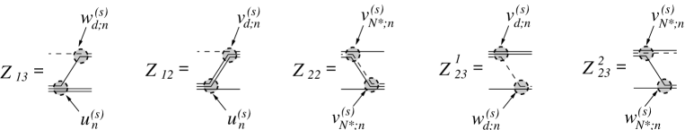
FIG. 2.: Diagrammatic representation of the potentials $Z_{\alpha\beta}$ in the separable approximation (see Appendix B).

FIG. 3.: Left panel: The leading eigenvalues of the Hilbert-Schmidt expansion for the three-nucleon scattering amplitude in the $S=T=1/2$ state. Right panel: The ratio between the Schmidt norms of the kernels ${\cal O}$ and ${\cal O}_{n}$ as defined by (45) and (46).

FIG. 4.: The same as in Fig. 3 for $\eta NN$-scattering in the $(S;T)=(1;0)$ state.

FIG. 5.: The same as in Fig. 3 for the $(\eta N)$+$(NN)$ partition.

FIG. 6.: Total cross section of elastic $\eta$-³H-scattering versus the c.m. kinetic energy $E$.

REFERENCES

• [1] J.C.Β Peng et al., Phys. Rev. Lett. 63, 2353 (1989).
• [2] B.Β Mayer et al., Phys. Rev.Β C 53, 2068 (1996).
• [3] B.Β Krusche, Contribution presented at Meson 2002, 7th International Workschop on Production, Properties and Interaction of Mesons (Cracow, Poland, May 24-28, 2002).
• [4] C.Β Wilkin, Phys. Rev.Β C 47, R938 (1993).
• [5] S.Β Wycech, A.M.Β Green, and J.A.Β Niskanen, Phys. Rev.Β C 52, 544 (1995).
• [6] V.B.Β Belyaev, S.A.Β Rakityansky, S.A.Β Sofianos, M.Β Braun, and W.Β Sandhas, Few Body Syst., Suppl.Β 8, 309 (1995). S.A.Β Rakityansky, S.A.Β Sofianos, M.Β Braun, V.B.Β Belyaev, and W.Β Sandhas, Phys. Rev.Β C 53, R2043 (1996).
• [7] N.V.Β Shevchenko, V.B.Β Belyaev, S.A.Β Rakityansky, S.A.Β Sofianos, and W.Β Sandhas, nucl-th/0108031.
• [8] K.P.Β Khemchandani, N.G.Β Kelkar, and B.K.Β Jain, nucl-th/0112065.
• [9] O.A.Β Yakubovsky, Yad. Fiz. 5, 1312 (1967) (Trans.: Sov. J. Nucl. Phys.Β 5, 937 (1967)).
• [10] L.D.Β Faddeev, Proc. First Int. Conf. on the Three-Body Problem, Birmingham, 1969, eds. J.S.C. McKee and P.M. Rolph (North-Holland, Amsterdam 1970).
• [11] P.Β Grassberger and W.Β Sandhas, Nucl. Phys.Β B2, 181 (1967).
• [12] E.O.Β Alt, P.Β Grassberger, and W.Β Sandhas, Phys. Rev.Β C 1, 85 (1970).
• [13] A.C.Β Fonseca, Proc.Β 8th Autumn School on Models and Methods in Few-Body Physics, Lisboa, 1986, eds. L.S.Β Ferreira, A.C.Β Fonseca and L.Β Streit, Lecture Notes in Physics 273, 161 (1986).
• [14] I.M.Β Narodetsky, Riv. Nuovo Cim.Β 4, 1 (1981).
• [15] J.A.Β Tjon, Phys. Lett.Β B56, 217 (1975); Phys. Lett.Β B63, 391 (1976).
• [16] A.C.Β Fonseca, Phys. Rev. Lett.Β 83, 4021 (1999).
• [17] F.Β Ciesielski, J.Β Carbonell, and C.Β Gignoux, Phys. Lett.Β B447, 199 (1999).
• [18] M.Β Viviany, A.Β Kievsky, S.Β Rosati, E.A.Β George, and L.D.Β Knutson, Phys. Rev. Lett.Β 86, 3739 (2001).
• [19] Y.Β Avishai and T.Β Mizutani, Nucl. Phys.Β A393, 429 (1983).
• [20] T.Β Ueda, Nucl. Phys.Β A505, 610 (1989).
• [21] L.Β Canton, Phys. Rev.Β C 58, 3121 (1998).
• [22] Y.Β Yamaguchi, Phys. Rev.Β C 95, 1628 (1954).
• [23] M.Β Batinic, I.Β Slaus, A.Β Svarc, and B.Β Nefkens, Phys. Rev.Β C 55, 2310 (1995).
• [24] A.M.Β Green and S.Β Wycech, Phys. Rev.Β C 55, R2167 (1997).
• [25] S.Β Weinberg, Phys. Rev.Β 133, B232 (1964).
• [26] A.G.Β Sitenko, Lectures in Scattering Theory (Pergamon Press, Oxford, 1974)
• [27] C.Β Lovelace, Phys. Rev.Β 135, B1225 (1964).
• [28] N.V.Β Shevchenko, S.A.Β Rakityansky, S.A.Β Sofianos, V.B.Β Belyaev, and W.Β Sandhas, Phys. Rev.Β C 58, R3055 (1998).
• [29] A.Β Fix and H.Β ArenhΓΆvel, Nucl. Phys. A697, 277 (2001).
• [30] A.M.Β Green and S.Β Wycech, Phys. Rev.Β C 64, 045206 (2001).
• [31] L.I.Β Schiff, Phys. Rev.Β 133, B802 (1964).
• [32] V.A.Β Tryasuchev, Yad. Fiz. 60, 245 (1997) (Trans.: Phys. Atom. Nucl.Β 60, 186 (1997)).
• [33] A.R.Β Edmonds, Angular Momentum in Quantum Mechanics (Princeton University Press, Princeton, New Jersey, 1957).