Lectures on Effective Field Theories for

Nuclei, Nuclear Matter and Dense Matter 
Mannque Rho

Service de Physique Théorique, CEA Saclay, 91191 Gif-sur-Yvette, France

and

School of Physics, Korea Institute for Advanced Study, Seoul 130-012, Korea

()

Abstract

This note is based on four lectures that I gave at the 10th Taiwan Nuclear Spring School held at Hualien, Taiwan in January 2002. It aims to correlate the old notion of Cheshire Cat Principle developed for elementary baryons to the modern notion of quark-baryon and gluon-meson “continuities” or “dualities” in dilute and dense many-body systems and predict what would happen to mesons when squeezed by nuclear matter to high density as possibly realized in compact stars. Using color-flavor locking in QCD, the vector mesons observed at low density can be described as the Higgsed gluons dressed by cloud of collective modes, i.e., pions just as they are in superdense matter, thus showing the equivalence between hidden $flavor$ gauge symmetry and explicit $color$ gauge symmetry. Instead of going into details of well-established facts, I focus on a variety of novel ideas – some solid and some less – that could be confirmed or ruled out in the near future.

1 INTRODUCTION

Let me begin with the question why do we need effective field theory (EFT in short) for nuclear physics? After all, there is quantum chromodynamics (QCD) with quarks and gluons figuring as microscopic degrees of freedom that is supposed to answer all the questions in the strong interactions, so why not just do QCD, the fundamental theory? The answer that everybody knows by now is a cliché: Nuclear physics involves the nonperturbative regime of QCD and cannot be accessed by a controlled method known up to date given in terms of the microscopic variables.

Next granted that EFT does mimic QCD in the nonperturbative regime, what then is the objective of doing effective field theories in nuclear physics?

In my opinion, there are, broadly speaking. two reasons for doing it. One is the obvious one often invoked: It is to confirm that nuclear physics is $indeed$ an integral part of the Standard Model, namely its strong interaction component (i.e., the $SU(3)_{c}$ gauge sector), thereby putting it on the same ground as that of EW particle physics ($SU(2)\times U(1)$). If an effective field theory were constructed in a way fully consistent with QCD, then it should describe nuclear processes as correctly and as accurately as dictated by QCD if one worked hard enough and computed all the things that are required within the given framework. We have seen how this works out in the case of $\pi$-$\pi$ scattering and $\pi$-$N$ scattering at low energies. Here one encounters neither puzzles nor any indication that something is going basically wrong that requires a new insight. I believe that the same will be the case with EFT’s in nuclear physics when things are developed well enough. It’s just a matter of hard work. Needless to say, we won’t be able to calculate everything that way in nuclear physics: Our computational power is simply too limited. However for processes that are accessible to a systematic EFT treatment, the procedure should work out all right.

To me, the more important raîson d’être of EFT in nuclear physics is two-fold: (1) to be able to make precise error-controlled calculations of certain processes important for fundamental issues of physics that cannot be provided by the standard nuclear physics approach (which I will call “SNPA”); (2) to make predictions, whether qualitative or quantitative, for processes that the SNPA cannot access, such as phase transitions under extreme conditions. If the EFT that we develop is to reproduce the fundamental theory and if the fundamental theory represents Nature, then the ultimate goal should be to make predictions that can in some sense be trusted and verified eventually. At present this aspect is not as widely recognized as it merits to be by the physics community.

In this series of lectures, I will develop the notion that when phrased in the EFT languages, the “old physics” encapsulated in SNPA and the “new physics” contained in QCD may be continuously connected. This notion will be developed in terms of a circle of “dualities” implicit in the phenomenon called “Cheshire Cat Principle.” I will try to develop the arguments that quarks in QCD are connected to baryons in hadronic spectrum and likewise gluons to mesons in the sense that a Cheshire-Cat phenomenon is operative.

2 Lecture I: The Cheshire Cat Principle

In this first lecture, I address the question: Are the low-energy properties of hadrons sensitive to the size of the region in which quarks and gluons of QCD are “confined”? The Cheshire Cat Principle (CCP) states that they should not be. The important point to underline here is that we are talking about how the degrees of freedom associated with the quarks and gluons are connected to the degrees of freedom associated with physical hadrons. The CCP addresses this problem in terms of the spaces occupied by the respective degrees of freedom [NRZ,RHO:PR]. It simply says that the naive picture of the “confinement” as understood in the old days of the MIT bag model is sometimes not correct. This point will appear later in a different context.

2.1 The Cheshire Cat Model in (1+1) Dimensions

Here, I will use a model to develop the picture, rather than a theory, of EFT. The aim is to describe the general theme that at low energies, the “confinement size” has no physical meaning in QCD. The thing we get out is that in terms of the space time, the region occupied by the microscopic variables of QCD, i.e., quarks and gluons, can be made big or small or shrunk to zero without affecting physics. Since doing this in four dimensions is quite difficult, I will do this in (1+1) dimension.

In two dimensions, the Cheshire Cat principle (CCP) can be formulated exactly. In the spirit of a chiral bag, consider a massless free single-flavored fermion $\psi$ confined in a region (“inside”) of “volume” $V$ coupled on the surface $\partial V$ to a free boson $\phi$ living in a region of “volume” $\tilde{V}$ (“outside”). We can think of the “inside” the line segment $x<R$ and the “outside” the line segment $x>R$ where $R$ is the “surface.” Of course in one-space dimension, the “volume” is just a segment of a line but we will use this symbol in analogy to higher dimensions. We will assume that the action is invariant under global chiral rotations and parity. Interactions invariant under these symmetries can be introduced without changing the physics, so the simple system that we consider captures all the essential points of the construction. The action contains three terms

$$S=S_{V}+S_{\tilde{V}}+S_{\partial V}$$ (2.1)

where

$$S_{V} = \int_{V}d^{2}x\bar{\psi}i\gamma^{\mu}\partial_{\mu}\psi+\cdots,$$ (2.2)

$$S_{\tilde{V}} = \int_{\tilde{V}}d^{2}x\frac{1}{2}(\partial_{\mu}\phi)^{2}+\cdots$$ (2.3)

and $S_{\partial V}$ is the boundary term which we will specify shortly. Here the ellipsis stands for other terms such as interactions, fermion masses etc. consistent with the assumed symmetries of the system on which we will comment later. For instance, there can be a coupling to a $U(1)$ gauge field in (2.2) and a boson mass term in (2.3) as would be needed in Schwinger model. Without loss of generality, we will simply ignore what is in the ellipsis unless we absolutely need it. Now the boundary term is essential in making the connection between the two regions. Its structure depends upon the physics ingredients we choose to incorporate.

Before going further, one caveat here. We will call $\phi$ the “pion.” Now in (1+1) dimensions, continuous symmetries do not spontaneously break, so there are no Goldstone bosons. One way to avoid this caveat is to think that one dimenional space is actually the radial coordinate of a sphere in 3-dimensional space. It is in this sense we will be talking about chiral symmetry.

We will assume that chiral symmetry holds on the boundary even if it is, as in Nature, broken both inside and outside by mass terms. As long as the symmetry breaking is gentle, this should be a good approximation since the surface term is a $\delta$ function. We should also assume that the boundary term does not break the discrete symmetries ${\cal P}$, ${\cal C}$ and ${\cal T}$. Finally we demand that it give no decoupled boundary conditions, that is to say, boundary conditions that involve only $\psi$ or $\phi$ fields. These three conditions are sufficient in (1+1) dimensions to give a unique term

$$S_{\partial V}=\int_{\partial V}d\Sigma^{\mu}\left\{\frac{1}{2}n_{\mu}\bar{\psi}e^{i\gamma_{5}\phi/f}\psi\right\}$$ (2.4)

with the $\phi$ “decay constant” $f=1/\sqrt{4\pi}$ where $d\Sigma^{\mu}$ is an area element with $n^{\mu}$ the normal vector, i.e, $n^{2}=-1$ and picked outward-normal. As we will mention later, we cannot establish the same unique relation in (3+1) dimensions but we will continue using this simple structure even when there is no rigorous justification in higher dimensions.

At classical level, the action (2.1) gives rise to the bag “confinement,” namely that inside the bag the fermion (which we shall call “quark” from now on) obeys

$$i\gamma^{\mu}\partial_{\mu}\psi=0$$ (2.5)

while the boson (which we will call “pion”) satisfies

$$\partial^{2}\phi=0$$ (2.6)

subject to the boundary conditions on $\partial V$

$$in^{\mu}\gamma_{\mu}\psi = -e^{i\gamma_{5}\phi/f}\psi,$$ (2.7)

$$n^{\mu}\partial_{\mu}\phi = f^{-1}\bar{\psi}(\frac{1}{2}n^{\mu}\gamma_{\mu}\gamma_{5})\psi.$$ (2.8)

Equation (2.7) is the familiar “MIT confinement condition” which is simply a statement of the classical conservation of the vector current $\partial_{\mu}j^{\mu}=0$ or $\bar{\psi}\frac{1}{2}n^{\mu}\gamma_{\mu}\psi=0$ at the surface while Eq. (2.8) is just the statement of the conserved axial vector current $\partial_{\mu}j_{5}^{\mu}=0$ (ignoring the possible explicit mass of the quark and the pion at the surface). The crucial point of our argument is that these classical observations are invalidated by quantum mechanical effects. In particular while the axial current continues to be conserved, the vector current fails to do so due to quantum anomaly.

There are several ways of seeing that something is amiss with the classical conservation law, with slightly different interpretations. The easiest way is as follows. Imagine that the quark is “confined” in the space $-\infty\leq r\leq R$ with a boundary at $r=R$. Now the vector current $j_{\mu}=\bar{\psi}\gamma_{\mu}\psi$ is conserved inside the “bag”

$$\partial^{\mu}j_{\mu}=0,\ \ \ \ \ r<R.$$ (2.9)

If one integrates this from $-\infty$ to $R$ in $r$, one gets the time-rate change of the fermion (i.e, quark) charge

$$\dot{Q}\equiv\frac{d}{dt}Q=2\int_{-\infty}^{R}dr\partial_{0}j_{0}=2\int_{-\infty}^{R}dr\partial_{1}j_{1}=2j_{1}(R)$$ (2.10)

which is just

$$\bar{\psi}n^{\mu}\gamma_{\mu}\psi,\ \ \ \ r=R.$$ (2.11)

This vanishes classically as we mentioned above. But this is not correct quantum mechanically because it is not well-defined locally in time. In other words, $\psi^{\dagger}(t)\psi(t+\epsilon)$ goes like $\epsilon^{-1}$ and so is singular as $\epsilon\rightarrow 0$. To circumvent this difficulty which is related to vacuum fluctuation, we regulate the bilinear product by point-splitting in time

$$j_{1}(t)=\bar{\psi}(t)\frac{1}{2}\gamma_{1}\psi(t+\epsilon),\ \ \ \ \ \epsilon\rightarrow 0.$$ (2.12)

Now using the boundary condition

$$i\gamma_{1}\psi(t+\epsilon) = e^{i\gamma_{5}\phi(t+\epsilon)/f}\psi(t+\epsilon)$$ (2.13)

$$\approx e^{i\gamma_{5}\phi(t)/f}[1+i\epsilon\gamma_{5}\dot{\phi}(t)/f]e^{\frac{1}{2}[\phi(t),\phi(t+\epsilon)]}\psi(t+\epsilon),\ \ \ \ r=R$$

and the commutation relation

$$[\phi(t),\phi(t+\epsilon)]=i\ {\rm sign}\ \epsilon,$$ (2.14)

we obtain

$$j_{1}(t)=-\frac{i}{4f}\epsilon\dot{\phi}(t)\psi^{\dagger}(t)\psi(t+\epsilon)=\frac{1}{4\pi f}\dot{\phi}(t)+O(\epsilon),\ \ \ \ r=R$$ (2.15)

where we have used $\psi^{\dagger}(t)\psi(t+\epsilon)=\frac{i}{\pi\epsilon}+[{\rm regular}]$. Thus quarks can flow out or in if the pion field varies in time. But by fiat, we declared that there be no quarks outside, so the question is what happens to the quarks when they leak out? They cannot simply disappear into nowhere if we impose that the fermion (quark) number is conserved. To understand what happens, rewrite (2.15) using the surface tangent

$$t^{\mu}=\epsilon^{\mu\nu}n_{\nu}.$$ (2.16)

We have

$$t\cdot\partial\phi=\frac{1}{2f}\bar{\psi}n\cdot\gamma\psi=\frac{1}{2f}\bar{\psi}t\cdot\gamma\gamma_{5}\psi,\ \ \ \ r=R$$ (2.17)

where we have used the relation $\bar{\psi}\gamma_{\mu}\gamma_{5}\psi=\epsilon_{\mu\nu}\bar{\psi}\gamma^{\nu}\psi$ valid in two dimensions. Equation (2.17) together with (2.8) is nothing but the bosonization relation

$$\partial_{\mu}\phi=f^{-1}\bar{\psi}(\frac{1}{2}\gamma_{\mu}\gamma_{5})\psi$$ (2.18)

at the point $r=R$ and time $t$. As is well known, this is a striking feature of (1+1) dimensional fields that makes one-to-one correspondence between fermions and bosons.

Equation (2.10) with (2.15) is the vector anomaly, i.e, quantum anomaly in the vector current: The vector current is not conserved due to quantum effects. What it says is that the vector charge which in this case is equivalent to the fermion (quark) number inside the bag is not conserved. Physically what happens is that the amount of fermion number $\Delta Q$ corresponding to $\Delta t\dot{\phi}/\pi f$ is pushed into the Dirac sea at the bag boundary and so is lost from inside and gets accumulated at the pion side of the bag wall. This accumulated baryon charge must be carried by something residing in the meson sector. Since there is nothing but “pions” outside, it must be be the pion field that carries the leaked charge. This means that the pion field supports a soliton. This is rather simple to verify in (1+1) dimensions. This can also be shown to be the case in (3+1) dimensions. In the present model, we find that one unit of fermion charge $Q=1$ is partitioned as

$$Q = 1=Q_{V}+Q_{\tilde{V}},$$ (2.19)

$$Q_{\tilde{V}} = \theta/\pi,$$

$$Q_{V} = 1-\theta/\pi$$

with

$$\theta=\phi(R)/f.$$ (2.20)

We thus learn that the quark charge is partitioned into the bag and outside of the bag, without however any dependence of the total on the size or location of the bag boundary. In (1+1)-dimensional case, one can calculate other physical quantities such as the energy, response functions and more generally, partition functions and show that the physics does not depend upon the presence of the bag. We could work with quarks alone, or pions alone or any mixture of the two. If one works with the quarks alone, we have to do a proper quantum treatment to obtain something which one can obtain in mean-field order with the pions alone. In some situations, the hybrid description is more economical than the pure ones. The complete independence of the physics on the bag – size or location– is called the “Cheshire Cat Principle” (CCP) with the corresponding mechanism referred to as “Cheshire Cat Mechanism” (CCM). Of course the CCP holds exactly in (1+1) dimensions because of the exact bosonization rule. There is no exact CCP in higher dimensions since fermion theories cannot be bosonized exactly in higher dimensions but a fairly strong case of CCP can be made for (3+1) dimensional models. Topological quantities like the fermion (quark or baryon) charge satisfy an exact CCP in (3+1) dimensions while nontopological observables such as masses, static properties and also some nonstatic properties satisfy it approximately but rather well.

So far we have been treating the quark as “colorless”, in other words, in the absence of a gauge field. Let us consider that the quark carries a $U(1)$ charge $e$, coupling to a $U(1)$ gauge field $A^{\mu}$. We will still continue working with a single-flavored quark, treating the multi-flavored case later. Then inside the bag, we have essentially the Schwinger model, namely, (1+1)-dimensional QED. It is well established that the charge is confined in the Schwinger model, so there are no charged particles in the spectrum. If now our “leaking” quark carries the color (electric) charge, this will at first sight pose a problem since the anomaly obtained above says that there will be a leakage of the charge by the rate

$$\dot{Q^{c}}=\frac{e}{2\pi}\dot{\phi}/f.$$ (2.21)

This means that the charge accumulated on the surface will be

$$\Delta Q^{c}=\frac{e}{2\pi}\phi(t,R)/f.$$ (2.22)

Unless this is compensated, we will have a violation of charge conservation, or breaking of gauge invariance. This is unacceptable. Therefore we are forced to introduce a boundary condition that compensates the induced charge, i.e, by adding a boundary term

$$\delta S_{\partial V}=-\int_{\partial V}d\Sigma\frac{e}{2\pi}\epsilon^{\mu\nu}n_{\nu}A_{\mu}\frac{\phi}{f}$$ (2.23)

with $n^{\mu}=g^{\mu\nu}n_{\nu}$. The action is now of the form

$$S=S_{V}+S_{\tilde{V}}+S_{\partial V}$$ (2.24)

with

$$S_{V} = \int_{V}d^{2}x\left\{\bar{\psi}(x)\left[i\partial_{\mu}-eA_{\mu}\right]\gamma^{\mu}\psi(x)-\frac{1}{4}F_{\mu\nu}F^{\mu\nu}\right\},$$ (2.25)

$$S_{\tilde{V}} = \int_{\tilde{V}}d^{2}x\left\{\frac{1}{2}(\partial_{\mu}\phi(x))^{2}-\frac{1}{2}m_{\phi}^{2}\phi(x)^{2}\right\},$$ (2.26)

$$S_{\partial V} = \int_{\partial V}d\Sigma\left\{\frac{1}{2}\bar{\psi}e^{i\gamma^{5}\phi/f}\psi-\frac{e}{2\pi}\epsilon^{\mu\nu}n_{\mu}A_{\nu}\frac{\phi}{f}\right\}.$$ (2.27)

We have included the mass of the $\phi$ field, the reason of which will become clear shortly.

In this example, we are having the “pion” field (more precisely the soliton component of it) carry the color charge. In general, though, the field that carries the color could be different from the field that carries the soliton. In fact, in (3+1) dimensions, it is the $\eta^{\prime}$ field that will be coupled to the gauge field (although $\eta^{\prime}$ is colorless) while it is the pion field that supports a soliton. But in (1+1) dimensions, the soliton is lodged in the $U(1)$ flavor sector (whereas in (3+1) dimensions, it is in $SU(n_{f})$ with $n_{f}\geq 2$). For simplicity, we will continue our discussion with this Lagrangian.

2.2 The Mass of the Scalar $\phi$

We now illustrate how one can calculate the mass of the $\phi$ field using the action (2.24) and the CCM following [NRWZ]. This exercise will help understand a similar calculation of the mass of the $\eta^{\prime}$ in (3+1) dimensions. The additional ingredient needed for this exercise is the $U_{A}(1)$ (Adler-Bell-Jackiw) anomaly which in (1+1) dimensions takes the form 

$$\partial_{\mu}j_{5}^{\mu}=-\frac{e}{4\pi}\epsilon_{\mu\nu}F^{\mu\nu}=-\frac{1}{2\pi}eE.$$ (2.28)

Instead of the configuration with the quarks confined in $r<R$, consider a small bag “inserted” into the static field configuration of the scalar field $\phi$ which we will now call $\eta^{\prime}$ in anticipation of the (3+1)-dimensional case we will consider later. Let the bag be put in $-\frac{R}{2}\leq r\leq\frac{R}{2}$. The CCP states that the physics should not depend on the size $R$, hence we can take it to be as small as we wish. If it is small, then the charge accumulated at the two boundaries will be $\pm\frac{e}{2\pi}\phi/f$. This means that the electric field generated inside the bag is

$$E=F_{01}=\frac{e}{2\pi}(\phi/f).$$ (2.29)

Therefore from the $U_{A}(1)$ anomaly (2.28), the axial charge created or destroyed (depending on the sign of the scalar field) in the static bag is

$$2\int_{V}dr\partial_{\mu}j_{5}^{\mu}=2(-j_{1}^{5}|_{\frac{R}{2}}+j_{1}^{5}|_{-\frac{R}{2}})=-\frac{e^{2}}{2\pi^{2}}(\phi/f)R.$$ (2.30)

From the bosonization condition (2.18), we have

$$2f\left(\partial_{1}\phi|_{\frac{R}{2}}-\partial_{1}\phi|_{-\frac{R}{2}}\right)=\frac{e^{2}}{2\pi^{2}}(\phi/f)R.$$ (2.31)

Now taking $R$ to be infinitesimal by the CCP, we have, on cancelling $R$ from both sides,

$$\partial^{2}\phi-\frac{e^{2}}{4\pi^{2}f^{2}}\phi=0$$ (2.32)

which then gives the mass, with $f^{-2}=4\pi$,

$$m_{\phi}^{2}=\frac{e^{2}}{\pi},$$ (2.33)

the well-known scalar mass in the Schwinger model which can also be obtained by bosonizing the $(QED)_{2}$. A completely parallel reasoning has been used to calculate the $\eta^{\prime}$ mass in (3+1) dimensions [NRWZ, NRZ].

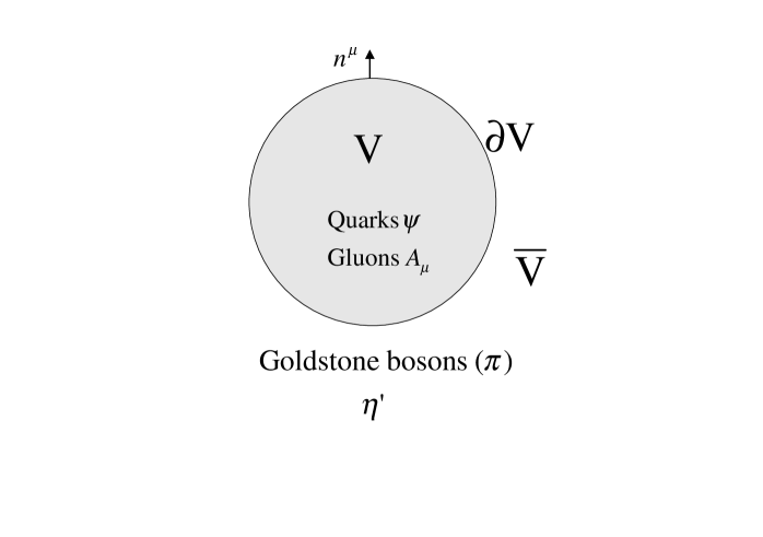
Figure 1: A spherical chiral bag for “deriving” a four-dimensional Cheshire Cat model. $\psi$ represents the doublet quark field of u and d quarks for $SU(2)$ flavor or the triplet of u, d and s for $SU(3)$ flavor and $\pi$ the triplet $\pi^{+},\pi^{-},\pi^{0}$ for $SU(2)$ and the octet pseudoscalars $\pi$, $K$, $\bar{K}$ and $\eta$ for $SU(3)$. The axial singlet meson $\eta^{\prime}$ figures in axial anomaly.

2.3 The Cheshire Cat Model in (3+1) Dimensions

Arguments paralleling the (1+1) dimensional model leads to the Lagrangian appropriate for (3+1) dimensions. We will just write it down and define the meanings of the terms involved. See [NRWZ, NRZ]. A cartoon of the model is given by Fig. 1.

$$S = S_{V}+S_{\tilde{V}}+S_{\partial V},$$ (2.34)

$$S_{V} = \int_{V}d^{4}x\left(\bar{\psi}i\not\!\!{D}\psi-\frac{1}{2}{\rm tr}\ F_{\mu\nu}F^{\mu\nu}\right)+\cdots$$

$$S_{\tilde{V}} = \frac{f^{2}}{4}\int_{\tilde{V}}d^{4}x\left({\mbox{Tr}}\ \partial_{\mu}U^{\dagger}\partial^{\mu}U+\frac{1}{4N_{f}}m^{2}_{\eta^{\prime}}({\rm ln}U-{\rm ln}U^{\dagger})^{2}\right)+\cdots+S_{WZW},$$

$$S_{\partial V} = \frac{1}{2}\int_{\partial V}d\Sigma^{\mu}\left\{(n_{\mu}\bar{\psi}U^{\gamma_{5}}\psi)+i\frac{g^{2}}{16\pi^{2}}{K_{5}}_{\mu}({\mbox{Tr}}\ {\rm ln}U^{\dagger}-{\mbox{Tr}}\ {\rm ln}U)\right\}.$$ (2.35)

Here $f$ is the pion decay constant $f\equiv f_{\pi}\sim 93$ MeV, $U$ is the unitary chiral field

$$U=e^{i\eta^{\prime}/f_{0}}e^{2i\pi/f},\ U^{\gamma_{5}}=e^{i\gamma_{5}\eta^{\prime}/f_{0}}e^{2i\gamma_{5}\pi/f}$$ (2.36)

$$f_{0}\equiv\sqrt{N_{f}/2}f,$$ (2.37)

$S_{WZW}$ is the Wess-Zumino-Witten term defined in the space-time volume $\tilde{V}$ and $K_{5\mu}$ is the Chern-Simons current

$$K_{5}^{\mu}=\epsilon^{\mu\nu\alpha\beta}(A_{\nu}^{a}F_{\alpha\beta}^{a}-\frac{2}{3}gf^{abc}A_{\nu}^{a}A_{\alpha}^{b}A_{\beta}^{c}).$$ (2.38)

If in accordance with the CCP one were to shrink the bag to a point, that is, let $R\rightarrow 0$, then one would be left over with only the meson fields. In terms of the $U$ field alone, this would be an infinite series in derivatives, the leading order terms taking the form

$$S = \frac{f^{2}}{4}\int_{V+\tilde{V}}d^{4}x{\mbox{Tr}}\ \partial_{\mu}U^{\dagger}\partial^{\mu}U+\cdots+S_{WZW}$$ (2.39)

with the WZW term defined in the whole space $(V+\tilde{V})$. The ellipsis stands for lots of higher order (higher derivative, mass etc.) terms which need to be included depending upon the processes treated. What comes out here is just the generalization of Skyrme-type theory, representing QCD at large $N_{c}$. One may introduce heavier meson fields replacing part of the ellipsis. In Lectures III and IV, the vector mesons $\rho$, $\omega$ will figure explicitly and play an important role. The part of the WZW term belonging to the volume $V$ arises through an interplay between anomalies inside $V$ and the surface terms as the volume $V$ is shrunk to a point and precisely makes up the complement to the WZW term of the volume $\tilde{V}$. How this comes about – which is quite intricate – is described in [NRZ].

The Lagrangian (2.34) has all the relevant symmetries and anomalies that should give a correct representation of QCD for large $N_{c}$. No one has yet fully studied the contents of this theory as there are certain aspects of the equations which have not been fully worked out. So far there is nothing which indicates that the CCP fails in Nature.

I don’t have the time for discussing it here but let me just mention that in the form (2.39), the effective Lagrangian should describe not only the baryons but also finite nuclei, nuclear matter and dense matter. The current development involves mainly classical solutions of the skyrmion-type theory for the systems with a finite number of baryons, i.e., “finite nuclei,” which are interesting from a mathematical point of view but do not resemble the real nuclei. It remains to be seen what happens when the solutions are quantized. An extremely interesting recent development is to study infinite matter within the Skyrme Lagrangian. Again this is at the classical level, with the discovery of a variety of crystal structures at “high density” ( see [PMRV, SCHWINDT] for a recent effort) but again it remains to be quantized. Approaching dense matter through the skyrmion matter is relevant to the study of phase structure of hadronic matter under compression needed for unravelling the structure of compact stars.

2.4 The “Proton Spin” Problem

The so-called “proton spin” problem had defied the CCP until recently and it is only now [LMPRV] that it is resolved within the framework of the CC model (2.34). This problem has been studied extensively not only in the context of hadronic models but also from the point of view of QCD proper. In fact there are many, most likely equivalent, ways, some more in line with QCD than others, but we will not go into this matter. The objective of the present discussion is not so much to “explain” the resolution of the problem but to illustrate the subtlety involved in the way the CC manifests in this problem.

Since the “proton spin” issue is connected with the flavor singlet axial matrix element $a_{0}$, we have to define what the current is in the chiral bag model (CBM) (2.34). We write the current in the CBM as a sum of two terms, one from the interior of the bag and the other from the outside populated by the meson field $\eta^{\prime}$ (how to account for the Goldstone pion fields is known; the mechanism is identical to what was described above in the context of the (1+1) dimensional picture and it will be taken into account for the baryon charge leakage)

$$A^{\mu}=A^{\mu}_{B}\Theta_{B}+A^{\mu}_{M}\Theta_{M}.$$ (2.40)

For notational simplicity, we will omit the flavor index in the current. We shall use the short-hand notations $\Theta_{B}=\theta(R-r)$ and $\Theta_{M}=\theta(r-R)$ with $R$ the radius of the bag. We interpret the $U_{A}(1)$ anomaly as given in this model by

$$\partial_{\mu}A^{\mu}=\frac{\alpha_{s}N_{F}}{2\pi}\sum_{a}\vec{E}^{a}\cdot\vec{B}^{a}\Theta_{B}+fm_{\eta}^{2}\eta\Theta_{M}.$$ (2.41)

We are assuming here that in the nonperturbative sector outside of the bag, the only relevant $U_{A}(1)$ degree of freedom is the massive $\eta^{\prime}$ field. This allows us to write

$$A^{\mu}_{M}=A^{\mu}_{\eta}=f\partial^{\mu}\eta$$ (2.42)

with the divergence

$$\partial_{\mu}A^{\mu}_{\eta}=fm_{\eta}^{2}\eta.$$ (2.43)

It turns out to be more convenient to write the current as

$$A^{\mu}=A_{B_{Q}}^{\mu}+A_{B_{G}}^{\mu}+A_{\eta}^{\mu}$$ (2.44)

such that

$$\partial_{\mu}(A_{B_{Q}}^{\mu}+A_{\eta}^{\mu}) = fm_{\eta}^{2}\eta\Theta_{M},$$ (2.45)

$$\partial_{\mu}A_{B_{G}}^{\mu} = \frac{\alpha_{s}N_{F}}{2\pi}\sum_{a}\vec{E}^{a}\cdot\vec{B}^{a}\Theta_{B}.$$ (2.46)

The subindices Q and G imply that these currents are written in terms of quark and gluon fields respectively. In writing (2.45), the up and down quark masses are ignored. Since we are dealing with an interacting theory, there is no unique way to separate the different contributions from the gluon, quark and $\eta$ components. In particular, the separation we adopt, (2.45) and (2.46), is neither unique nor gauge invariant although the sum is without ambiguity. This separation, however, is found to lead to a natural partition of the contributions in the framework of the bag description for the confinement mechanism that is used here.

We now discuss individual contributions from each term.

$\bullet$ The quark current $A_{B_{Q}}^{\mu}$

The quark current is given by

$$A^{\mu}_{B_{Q}}=\bar{\Psi}\gamma^{\mu}\gamma_{5}\Psi$$ (2.47)

where $\Psi$ should be understood to be the bagged quark field. Therefore the quark current contribution to the FSAC is given by

$$a^{0}_{B_{Q}}=\langle p|\int_{B}d^{3}r\bar{\Psi}\gamma_{3}\gamma_{5}\Psi|p\rangle.$$ (2.48)

The calculation of this type of matrix elements in the CBM is nontrivial due to the baryon charge leakage between the interior and the exterior through the Dirac sea. But we know how to do this in an unambiguous way. A complete account of such calculations and references can be found in the literature [RHO:PR, NRZ]. The leakage produces an $R$ dependence which would otherwise be absent. One finds that there is no contribution for zero radius, that is in the pure skyrmion scenario for the proton. The contribution grows as a function of $R$ towards the pure MIT result although it may never reach it even at infinite radius.

$\bullet$ The meson current $A^{\mu}_{\eta}$

Due to the coupling of the quark and $\eta$ fields at the surface, we can simply write the $\eta$ contribution in terms of the quark contribution,

$$a^{0}_{\eta}=\frac{1+y_{\eta}}{2(1+y_{\eta})+y_{\eta}^{2}}\langle p|\int_{B}d^{3}r\bar{\Psi}\gamma_{3}\gamma_{5}\Psi|p\rangle.$$ (2.49)

where $y_{\eta}=m_{\eta}R$. Since the $\eta$ field has no topological structure, its contribution also vanishes in the skyrmion limit. Due to baryon charge leakage, however, this contribution increases slowly as the bag increases. This illustrates how the dynamics of the exterior can be mapped to that of the interior by boundary conditions. We may summarize the analysis of these two contributions by stating that no trace of the CCP is apparent from the “matter” contribution. As shown in Fig. 2, there is a sensitive dependence on $R$. Thus if the CCP were to emerge, the only possibility would be that the gluons do the miracle!

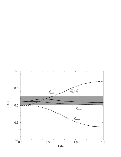
Figure 2: Various contributions to the flavor singlet axial current of the proton as a function of bag radius and comparison with the experiment: (a) quark plus $\eta$ (or “matter”) contribution ($a^{0}_{B_{Q}}+a^{0}_{\eta}$), (b) the contribution of the static gluons due to quark source ($a^{0}_{G,stat}$), (c) the gluon Casimir contribution ($a^{0}_{G,vac}$), and (d) their sum ($a^{0}_{total})$. The shaded area corresponds to the range admitted by experiments.

Let us turn to the gluon contribution. The gluon current is split into two pieces

$$A^{\mu}_{B_{G}}=A^{\mu}_{G,stat}+A^{\mu}_{G,vac}.$$ (2.50)

The first term arises from the quark and $\eta$ sources, while the latter is associated with the properties of the vacuum of the model. One might worry that this contribution could not be split in these two terms without double counting. However this worry is unfounded. Technically, it is easy to check it by noticing that the former acts on the quark Fock space and the latter on the gluon vacuum. Thus, one can interpret the former as a one gluon exchange correction to the quantity. One can also show this intuitively by making the analogy to the condensate expansion in QCD, where the perturbative terms and the vacuum condensates enter additively to the lowest order.

$\bullet$ The gluon static current $A^{\mu}_{G,stat}$

Let us first describe the static term.

To the leading order, we can the $\eta$ coupling. Afterwards, the $\eta$ contribution can be added. The boundary conditions for the gluon field would correspond to the original MIT ones. The quark current is the source term that remains in the equations of motion after performing a perturbative expansion in the QCD coupling constant, i.e., the quark color current

$$g{\bar{\Psi}}_{0}\gamma_{\mu}\lambda^{a}\Psi_{0}$$ (2.51)

where the $\Psi_{0}$ fields represent the lowest cavity modes. In this lowest mode approximation, the color electric and magnetic fields are given by

$$\vec{E}^{a}=g_{s}\frac{\lambda^{a}}{4\pi}\frac{\hat{r}}{r^{2}}\rho(r)$$ (2.52)

$$\vec{B}^{a}=g_{s}\frac{\lambda^{a}}{4\pi}\left(\frac{\mu(r)}{r^{3}}(3\hat{r}\vec{\sigma}\cdot\hat{r}-\vec{\sigma})+(\frac{\mu(R)}{R^{3}}+2M(r))\vec{\sigma}\right)$$ (2.53)

where $\rho$ is related to the quark density $\rho^{\prime}$ as

$$\rho(r,\Gamma)=\int_{\Gamma}^{r}ds\rho^{\prime}(s)$$

and $\mu,M$ to the vector current density

$$\mu(r) = \int_{0}^{r}ds\mu^{\prime}(s),$$

$$M(r) = \int_{r}^{R}ds\frac{\mu^{\prime}(s)}{s^{3}}.$$

The lower limit $\Gamma$ is taken to be zero in the MIT bag model – in which case the boundary condition is satisfied only globally, that is, after averaging – and $\Gamma=R$ in the so called monopole solution – in which case, the boundary condition is satisfied locally. We take the latter since consistency with the CCP condition rules out the MIT condition.

We now proceed to introduce the $\eta$ field. We perform the same calculation with however the color boundary conditions coming from (2.34) – which are modified by the color anomaly from the MIT ones – taken into account. In the approximation of keeping the lowest non-trivial terms, the boundary conditions become

$$\hat{r}\cdot\vec{E}_{stat}^{a}=\frac{N_{F}g^{2}}{8\pi^{2}f}\hat{r}\cdot\vec{B}^{a}_{g}\eta(R)$$ (2.54)

$$\hat{r}\times\vec{B}_{stat}^{a}=-\frac{N_{F}g^{2}}{8\pi^{2}f}\hat{r}\times\vec{E}^{a}_{g}\eta(R).$$ (2.55)

Here $\vec{E}^{a}_{g}$ and $\vec{B}^{a}_{g}$ are the lowest order fields given by (2.52) and (2.53) and $\eta(R)$ is the meson field at the boundary. The $\eta$ field is given by

$$\eta(\vec{r})=-\frac{g_{NN\eta}}{4\pi M}\vec{S}\cdot\hat{r}\frac{1+m_{\eta}r}{r^{2}}e^{-m_{\eta}r}$$ (2.56)

where the coupling constant is determined from the surface conditions.

Note that the magnetic field is not affected by the new boundary conditions, since $\vec{E}^{a}_{g}$ points into the radial direction. The effect on the electric field is just a change in the charge, i.e.,

$$\rho_{stat}(r)=\rho(r,\Gamma)+\rho_{\eta}(R)$$ (2.57)

where

$$\rho_{\eta}(R)=\frac{N_{F}g^{2}}{64\pi^{3}M}\frac{g_{NN\eta}}{f}(1+y_{\eta})e^{-y_{\eta}}.$$ (2.58)

The contribution to the FSAC arising from these fields is determined from the expectation value of the anomaly

$$a^{0}_{G,stat}=\langle p|-\frac{N_{F}\alpha_{s}}{\pi}\int_{B}d^{3}rx_{3}\vec{E}^{a}_{stat}\cdot\vec{B}^{a}_{stat}|p\rangle.$$ (2.59)

One finds that including the $\eta$ contribution in $\rho_{stat}(r)$ brings a non-negligible modification to the FSAC but does not modify the result qualitatively. The result as one can see in Fig. 2 shows that this contribution is zero at $R=0$ but increases as $R$ increases but with the sign opposite to that of the matter field, largely cancelling the $R$ dependence of the matter contribution. We should remark here that there is a drastic difference between the effect of the MIT-like electric field and that of the monopole-like electric field: The former is totally incompatible with the Cheshire Cat property whereas the latter remains consistent independently of whether or not the $\eta$ contribution is included in $\rho_{stat}$.

$\bullet$ The gluon Casimir current $A^{\mu}_{G,vac}$

Up to this point, the FSAC is zero for $R=0$ and non-zero for $R\neq 0$. This is in principle a violation of the CCP although the magnitude of the violation may be small. We now show that it is the vacuum contribution through Casimir effects that the CCP is restored. The calculation is subtle involving renormalization of the Casimir effects, the details of which are to be found in the paper by Lee et al. [LMPRV]. Here we summarize the salient feature of the contribution.

The quantity to calculate is the gluon vacuum contribution to the flavor singlet axial current of the proton, which can be done by evaluating the expectation value

$$\langle 0_{B}|-\frac{N_{F}\alpha_{s}}{\pi}\int_{V}d^{3}rx_{3}(\vec{E}^{a}\cdot\vec{B}^{a})|0_{B}\rangle$$ (2.60)

where $|0_{B}\rangle$ denotes the vacuum in the bag. To calculate this, we invoke at this point the CCP which states that at low energy, hadronic phenomena do not discriminate between QCD degrees of freedom (quarks and gluons) on the one hand and meson degrees of freedom (pions, etas,…) on the other, provided that all necessary quantum effects (e.g., quantum anomalies) are properly taken into account. If we consider the limit where the $\eta$ excitation is a long wavelength oscillation of zero frequency, the CCP asserts that it does not matter whether we choose to describe the $\eta$, in the interior of the infinitesimal bag, in terms of quarks and gluons or in terms of mesonic degrees of freedom. This statement, together with the color boundary conditions, leads to an extremely simple and useful local formula,

$$\vec{E}^{a}\cdot\vec{B}^{a}\approx-\frac{N_{F}g^{2}}{8\pi^{2}}\frac{\eta}{f}\frac{1}{2}G^{2},$$ (2.61)

where only the term up to the first order in $\eta$ is retained in the right-hand side. Here we adapt this formula to the CBM. This means that the couplings are to be understood as the average bag couplings and the gluon fields are to be expressed in the cavity vacuum through a mode expansion. That the surface boundary condition can be interpreted as a local operator is a rather strong CCP assumption which while justifiable for small bag radius, can only be validated à posteriori by the consistency of the result. This procedure is the substitute to the condensates in the conventional discussion.

Substituting Eq.(2.61) into Eq.(2.60) we obtain

$$\hskip-20.00003pt\langle 0_{B}|-\frac{N_{F}\alpha_{s}}{\pi}\int_{V}d^{3}rx_{3}(\vec{E}^{a}\cdot\vec{B}^{a})|0_{B}\rangle$$

$$\approx\left(-\frac{N_{F}\alpha_{s}}{\pi}\right)\left(-\frac{N_{F}g^{2}}{8\pi^{2}}\right)\frac{y(R)}{f_{0}}\langle p|S_{3}|p\rangle(N_{c}^{2}-1)$$

$$\hskip 30.00005pt\sum_{n}\int_{V}d^{3}r(\vec{B}_{n}^{*}\cdot\vec{B}_{n}-\vec{E}_{n}^{*}\cdot\vec{E}_{n})x_{3}\hat{x}_{3},$$ (2.62)

where we have used that $\eta$ has a structure of $(\vec{S}\cdot\hat{r})y(R)$. Since we are interested only in the first order perturbation, the field operator can be expanded by using MIT bag eigenmodes (the zeroth order solution). Thus, the summation runs over all the classical MIT bag eigenmodes. The factor $(N_{c}^{2}-1)$ comes from the sum over the abelianized gluons.

The next steps are the numerical calculations to evaluate the mode sum appearing in Eq.(2.62): (i) introduction of the heat kernel regularization factor to classify the divergences appearing in the sum and (ii) subtraction of the ultraviolet divergences. These procedures – which involve an intricate manipulation – are described in [LMPRV]. The result is shown in Fig. 2. Though the magnitude is small compared with the others, it is important at small $R$ to restore, within the CBM scheme, the CCP. The net result which is small due to the intricate cancellation between the matter contribution and the gluon contribution compares well with the experimental range quoted in the literature.

The lesson from this calculation is that neither the matter contribution nor the gluon contribution to $a^{0}$, both of which are gauge-non-invariant and CCP-violating, is physical. Only the total which is gauge invariant is physical and CCP-preserving.

3 Lecture II: Effective Field Theories for Dilute Matter and Superdense Matter

3.1 Strategy of EFT

I will start by briefly stating the principal idea of EFT relevant for low-energy processes that we will be considering. This is a nutshell presentation.

Picking a scale given by the cutoff $\Lambda$, one first divides a generic field $\Phi$ – that consists of $all$ degrees of freedom, bosonic as well fermionic – into the “high” field $\Phi_{H}$ lying above $\Lambda$ and the “low” field $\Phi_{L}$ lying below $\Lambda$, i.e., $\Phi=\Phi_{H}+\Phi_{L}$ and integrate out from the generating functional or partition function $Z$ the “high” component (in which we are not specifically interested) and write $Z$ in terms of $\Phi_{L}$ only. Defining the action in Euclidean space as

$$S[\Phi]=S_{0}[\Phi_{L}]+S_{0}[\Phi_{H}]+S_{I}[\Phi_{L},\Phi_{H}]$$ (3.1)

where $S_{0}$ stands for the non-interacting part of the action and $S_{I}$ for the interaction part, one writes

$$Z=\int[d\Phi_{L}]{\mbox{e}}^{-S^{eff}[\Phi_{L}]}$$ (3.2)

where

$$e^{-S^{eff}[\Phi_{L}]}=e^{-S_{0}[\Phi_{L}]}\int[d\Phi_{H}]e^{-S_{0}[\Phi_{H}]}e^{-S_{I}[\Phi_{L},\Phi_{H}]}.$$ (3.3)

This defines the mode elimination referred to as “decimation.” The next step is to write $S^{eff}$ in terms of integrals over local fields

$$S^{eff}[\Phi_{L}]=\int^{\Lambda}\sum_{i}C_{i}(\Lambda)Q_{i}$$ (3.4)

where $Q_{i}$ are polynomials of the local $\Phi_{L}$ fields. It should be emphasized that in general, when certain fields are integrated out, the resulting effective action is not always local, so in some cases (as discussed later), the localization can be a bad approximation. For the moment we will proceed assuming that the localization can be done.

There are typically two ways that the expansion (3.4) can be effectuated. If one has a theory that is well defined above and below $\Lambda$, i.e., over the whole space (like QED taken as a fundamental theory, not in a context of an effective theory that unifies all the interactions), then one can compute the coefficients $C_{i}$ as a function of $\Lambda$ from the theory. QCD that concerns us is not like this. Although QCD is a full theory by itself, the two regimes, above and below $\Lambda$, are not simply describable in terms of the same degrees of freedom. For instance, in the approach we will take, we imagine the degrees of freedom above $\Lambda$ to be given in terms of the microscopic variables, quarks and gluons, and those below $\Lambda$ by hadrons. In this case, we cannot simply compute the coefficients $C_{i}$ from theory (except perhaps on lattice) but we have to resort to experiments. In doing this, one has to inject a certain dose of intuition and guessing. The major task in doing this is to assess and minimize the errors committed in truncating the series.

The next thing to do is to do the scale counting in writing down the series (3.4). Given an action in D dimensions

$$S^{eff}=\int d^{D}x{{\cal L}}^{eff}$$ (3.5)

with the effective Lagrangian expressed in terms of the naive dimension of the field operators as

$${{\cal L}}^{eff}={\cal L}_{\leq D}+{\cal L}_{D+1}+{\cal L}_{D+2}+\cdots$$ (3.6)

one identifies the term ${\cal L}_{\leq D}$ to be “naively renormalizable” and all the rest “naively non-renormaiizable.” They have the following scaling property. To be specific, consider the scalar field theory

$$S=\int d^{D}x\left\{\frac{1}{2}(\partial_{\mu}\phi)^{2}-\frac{1}{2}m^{2}\phi^{2}+a\phi^{4}+b\phi^{6}+\cdots\right\}.$$ (3.7)

We want to determine how each operator in the action scales when one scales the space-time $x$,

$$x\rightarrow sx,\ \ \ s>1.$$ (3.8)

To do this, we have to define the standard measure. We do this by decreeing that the kinetic term in the action remains unscaled under (3.8). Now since $\partial\rightarrow s^{-1}\partial$, we have

$$\int d^{D}x(\partial_{\mu}\phi)^{2}\rightarrow s^{D-2+2[\phi]}\int d^{D}x(\partial_{\mu}\phi)^{2}.$$ (3.9)

We want this term unchanged, so for $D=4$, we find that $[\phi]=-1$. Such a term that remains unchanged under scaling is referred to as “marginal.”

Now the rest follows immediately. The $\Phi^{4}$ term is also marginal. The mass term scales as $s^{D-2}=s^{2}$. Terms scaling as $s^{n}$ with $n>0$ are referred to as “relevant.” The $\phi^{6}$ term goes as $s^{-2}$ etc. Terms scaling as $s^{m}$ with $m<0$ are called “irrelevant.” What these terms mean physically is that as the probe momentum/energy goes down, that is, as $s\rightarrow\infty$, marginal terms remain unchanged, irrelevant terms die away and relevant terms blow up.” Something unusual happens when the relevant terms take over and that something is related to phase transitions. Interesting physics can be lodged in the irrelevant terms although they get suppressed at low energy. In nuclear physics, as we will see later (e.g., the solar $pp$ and $hep$ processes), what nuclear physicists have been calling “short-range correlations” can be identified in the irrelevant terms in the action.

The next step is then to sum the series (3.4) including loop graphs of the same power counting. In doing this, the coefficients $C_{i}$ enter as counter terms to do the renormalization.

Suppose now we have the series. The given generating functional (or partition function) $Z$ then gives physical amplitudes ${{\cal A}}$. Since where one puts the cutoff is arbitrary, physical amplitudes should not depend upon what specific $\Lambda$ one chooses, assuming of course one knows how to pick all necessary degrees of freedom. This gives rise to the renormalization-group (RG) invariance,

$$d{\cal A}/d\Lambda=0$$ (3.10)

which leads to a relation for the coefficients $C_{i}$

$$dC_{i}(\Lambda)/d\Lambda={\cal F}_{i}(\Lambda)$$ (3.11)

where ${\cal F}_{i}$ are given functions of $\Lambda$. These are the renormalization group equations, known as Wilson equations or Callan-Symanzik equations depending upon what kind of theory one is dealing with. Our formulation given below is closer to the Wilsonian approach.

I have been describing the procedure in too general a term to this point. Let me be somewhat more specific so the discussion given later on the RG flows of hidden local symmetry (HLS) theory can be understandable. Suppose that $\Phi_{L}$ consists of a set of, say, three fields labelled $\phi_{A},\phi_{B},\phi_{C}$ defined at a scale $\Lambda_{a}$, i.e., $(\phi_{A},\phi_{B},\phi_{C})\in\Phi_{L}$. Now imagine that we are decimating the degrees of freedom from $\Lambda_{a}$ down to $\Lambda_{b}<\Lambda_{a}$ at which point the field $\phi_{A}$ decouples. All three fields $\phi_{A,B,C}$ contribute to the flows in this range. Next as one decimates from $\Lambda_{b}$ to $\Lambda_{c}<\Lambda_{b}$ at which point the field $\phi_{B}$ decouples, only $\phi_{B}$ and $\phi_{C}$ will contribute to the flow. From $\Lambda_{c}$ down, then only $\phi_{c}$ will contribute to the flow etc. Thus while one is lowering the cutoff in terms of energy/momentym scale, one is also “integrating out” associated degrees of freedom. In the next lecture, we will see that the various RG scales are intricately tied to the external disturbances such as density and/or temperature (i.e., density/temperature dependence of the RG scales) and one has to keep track of how the scales vary as a function of density/temperature in following the flows.

It turns out in certain cases that the right-hand side of (3.11) vanishes. In this case, we have a set of “fixed points.” The variety of fixed points, e.g., conformal fixed point, vector manifestation (VM) fixed point, Fermi-liquid fixed point etc., will play a primordial role in our developments.

3.2 EFT for Two-Nucleon Systems

As the first case, let us consider two-nucleon systems at very low energy. These systems are very well understood in the SNPA and as such, we will learn nothing new from the discussion given in this subsection as far physics as is concerned. However we do gain some insight as to how EFT works in the regime where things are well understood.

For low energy nuclear physics, the relevant degrees of freedom are the local fields of proton, neutron and pions. We imagine that all other degrees of freedom have been integrated out, with their imprints left in the higher-dimension terms. Thus the field spaces are

$$(n,p,\pi) \in \Phi_{L},$$

$$(\rho,\omega,a_{1},\Delta,\ {\rm glueballs},\cdots,J/\psi,\cdots) \in \Phi_{H}.$$ (3.12)

In this case, the series $C_{i}Q_{i}$ in (3.4) takes the form

$$f_{\pi}^{2}\Lambda^{2}(\pi/f_{\pi})^{m}(\partial/\Lambda)^{n}(N/f_{\pi}\sqrt{\Lambda})^{r}$$ (3.13)

where $f_{\pi}$ is the pion decay constant and $\Lambda$ here is the chiral cutoff $\sim 4\pi f_{\pi}\sim 1$ GeV. Chiral perturbation theory for pion-nucleon interactions is developed with this series in terms of the power ${\cal N}=m+n+r$.

If we further restrict ourselves to energy or momentum much less than the pion mass scale, we can even integrate out the pions as well. See [BEANE]. This is not a very good idea, however, if one wants to study response functions of two-nucleon (as well as multi-nucleon) systems (due to what is known as “chiral filter mechanism” in nuclei) as we will do in the next subsection where we will keep the pion fields explicitly. But for the discussion at hand, namely, S-wave scattering of two nucleons, eliminating the pions is justified. Treating the nucleon as nonrelativistic, the effective Lagrangian can be written as

$${\cal L}^{eff}=N^{\dagger}\left(i\partial_{t}+\frac{\vec{\nabla}^{2}}{2M}\right)-\frac{1}{2}[C^{s}(N^{\dagger}N)^{2}+C^{t}(N^{\dagger}\vec{\sigma}N)^{2}]+\cdots$$ (3.14)

where $M$ is the nucleon mass, the $C$’s are unknown constants to be fixed from experiments, and the ellipsis stands for higher nucleon fields and/or higher derivative terms. We shall ignore these higher dimension terms for the discussion.

Given the Lagrangian (3.14), one can do the standard calculation in terms of a Schrödinger equation provided the four-Fermi contact term is suitably regularized. One can also calculate an infinite set of Feynman diagrams and sum them. The latter is totally equivalent to the former (see [PKMR:CO]). It is however more transparent to do the latter. Summing the Feynman graphs of Fig. 3 to all orders, one gets the amplitude

$${\cal A}=-\frac{C}{1-C(GG)}$$ (3.15)

where $(GG)$ stands for the two-nucleon propagators which in the CM frame is

$$(GG)=\int\frac{d^{3}q}{(2\pi)^{3}}\frac{1}{E-q^{2}/M+i\epsilon}$$ (3.16)

with $\sqrt{ME}=|\vec{k}|\equiv k$.

Figure 3: Feynman graphs for nucleon-nucleon scattering via the four-nucleon contact interaction Lagrangian.

The integral (3.16) diverges, so needs to be regularized. We cut the integral at $\Lambda$ – to be specified below – and obtain 

$$(GG)=-\frac{M}{4\pi}\left(\frac{\Lambda}{\pi}+ik\right).$$ (3.17)

Thus

$${\cal A}=-\frac{C}{1+\frac{CM}{4\pi}(\frac{\Lambda}{\pi}+ik)}.$$ (3.18)

In general the coefficient $C$ will depend on where the cutoff $\Lambda$ is put. For a given $\Lambda$ it may be obtained from lattice. Unfortunately, we have no data on this. So we will resort to experiments to fix it. To do this, we write the amplitude in terms of the S-wave phase shift $\delta$,

$${\cal A}=\frac{4\pi}{M}\frac{1}{k\cot\delta-ik}\approx-\frac{4\pi}{M}\frac{1}{\frac{1}{a}+ik}$$ (3.19)

where the second approximate equality comes from the effective range formula, $k\cot\delta=-1/a+\frac{1}{2}r_{0}k^{2}+{\cal O}(k^{4})$. Comparing (3.18) and (3.19), we get

$$C(\Lambda)=\frac{4\pi}{M}\left(\frac{1}{-\frac{\Lambda}{\pi}+1/a}\right).$$ (3.20)

Note that the amplitude (3.18) with (3.20) satisfies the RG invariance condition $\Lambda\frac{d{\cal A}^{-1}}{d\Lambda}=0$ as it should.

What is interesting with this formula is that in Nature, the scattering length is huge compared with the typical hadronic scale $\sim 0.2$ fm and also with the cutoff scale which is expected to be of order $\sim(3m_{\pi})^{-1}$ so the $1/a$ term in (3.20) plays an unimportant role. Let us assume that the scattering length is infinite. Then we see that [MEHEN, BEANE]

$$\frac{d[\Lambda C(\Lambda)]}{d\Lambda}=0.$$ (3.21)

This means that there is a fixed point, called “scale invariant fixed point.”  To see that the theory for $a=\infty$ is scale-invariant, one notes that the four-Fermi interaction Lagrangian becomes ${\cal L}_{4fermi}=-\frac{2\pi}{M\Lambda}(N^{\dagger}N)^{2}$, so the action remains invariant under the scale change $\Lambda\rightarrow s^{-1}\Lambda$ and $N\rightarrow s^{-3/2}N$.

What’s the big deal with the scale invariance of the theory? It means that the S-wave nucleon-nucleon interaction at low energy is dominated by the scale-invariant fixed point. So it makes a good sense to fluctuate around this fixed point to do two-nucleon physics at low energy. But was it essential for describing two-nucleon interactions to know that there is such a fixed point? The answer is no. Nuclear physicists who knew nothing about it have been doing precision nuclear physics all along and got the right answers that can be compared with experiments.

I should note that as I did here with the cutoff regularization, there is nothing so special about the large scattering length. It is only in doing naive dimensional regularization that all sorts of bizarre things are encountered. Clearly were the $\Lambda$ term in (3.20) absent as in naive DR, the coefficient $C$ would be “unnaturally” big and the expansion would make no sense. This led some people to think that an EFT in nuclear physics needed new ingredient. But it is the naive regularization that is at fault, not the EFT: there is nothing that indicates that EFT is sick, in whatever form the EFT was formulated. This point is discussed in [PKMR:CO].

What about the pions? The pions are found to be somewhat awkward in keeping the counting kosher and some people attempted to treat the pions as perturbative. This may be OK for some low-energy scattering but treating the pions perturbatively not only spoils chiral invariance but also makes certain problems needlessly harder if not impossible. We know that the pion is essential for the deuteron structure. For one thing, the torus structure implied by the pion tensor force – which is visible experimentally, e.g., through electron scattering – cannot possibly be brought in by perturbation. Furthermore the “chiral filter mechanism” mentioned below [KDR] works marvellously well whenever soft-pion mechanisms are operative and guide us how to do a model-independent calculation even when they are not operative. The pion enters indispensably in this story which is the topic of the next subsection.

3.3 Predictive EFT

As I mentioned before, one of the objectives of doing EFT is to confirm that one can do a systematic calculation that is consistent with QCD of nuclear properties. One can for instance work out nuclear forces – nucleon-nucleon as well as multi-nucleon – to as high an order in the EFT counting as possible. This may be possible for two-nucleon interactions and perhaps eventually three-nucleon interactions. But physics-wise, it seems to me that the best one can hope to achieve here is to arrive at the accuracy obtained by those accurate phenomenological potentials available in the literature. It is possible and perhaps instructive to gauge the consistency of the methods used by the standard nuclear physics approach (SNPA) but I do not see what new physics can be learned from such hard work. It will of course be gratifying to verify that “nuclear physicists knew what they were doing and that they were doing it correctly.” The bottom line is that the harder one works here, the better it will come close to the phenomenological results. The most up-to-date effort in this direction can be found in [EPEL1,EPEL2].

I believe that it is in making $predictions$ – and not struggling with parameter-full exercises – that cannot be made by the SNPA in which the real power of EFT lies. After all, that is the ultimate objective of a fundamental theory, a feat that cannot be expected of models.

3.3.1 Chiral filter mechanism

I will follow Weinberg’s original chiral perturbation scheme in which the pion is put on the same footing as contact non-derivative four-nucleon interactions with the pion mass incorporated by means of perturbative unitarity. There is a bit of problem with the power counting when the pion is present ab initio and this has been discussed extensively by several people [BEANE]. I would not like to get into that matter as I believe it is a technical matter that does not seem to be important in most of the processes considered so far.

I will take it for granted that a sophisticated phenomenology with light nuclei can supply us accurate wave functions with which one can calculate response functions. Although $n$-body potentials for $n>2$ cannot be unambiguously determined in this way, two-body and possibly three-body potentials could be determined with great accuracy. And there is a growing evidence that this is the case. Solving the Schrödinger equation with such potentials corresponds to summing to all orders a subset of “reducible graphs” in the EFT expansion, with the “irreducible graphs” subsumed to be taken into account in the “accurate potentials” up to some high order. In exploiting these accurate wave functions that emerge from such calculations in the context of an EFT, it would of course be great to have a clear idea what is included and what is not included in the potentials used. In some cases, one of which is discussed here, this is possible. Now given such wave functions, can one calculate response functions measured in precision experiments as accurately as possible with the possibility of controlling the theoretical errors one commits ? This question can be answered affirmatively for the calculation of responses to slowly-varying EW fields.

Consider the matrix element of the vector current $J_{\mu}^{a}$ and the axial-vector current $J_{5\mu}^{a}$. We are interested in calculating $\langle f|J_{\mu}|i\rangle$ where $i$ and $f$ denote respectively the initial and final nuclear states. This current effective in $A$-body system can be decomposed into

$$J_{\mu}=\sum_{n=1}^{A}J_{\mu}^{(n)}.$$ (3.22)

Customarily, except for unusual cases, an example of which we will enocunter below, one-body terms are leading in the power counting (chiral counting in chiral-invariant theories) – and they $are$ numerically, so the theorist’s task is to compute the matrix elements of higher-body currents. Since the EW current will act only once for very weak and slowly-varying interactions, it suffices to systematically count the chiral orders of the irreducible graphs contributing to the current. This program was initiated many years ago [CR:71]. In terms of exchanges of mesons between the nucleons in interaction, the dominant “correction” to the leading one-body is the 2-body contribution with the exchange of one soft-pion in Fig. 4.

Figure 4: Two-body currents with one soft-pion exchange which dominate whenever unsuppressed by kinematics or symmetry. The cross stands for the current. Both (a) and (b) contribute to the vector current but only (a) contributes to the axial current.

The chiraL filter mechanism states [KDR] that whenever the one soft-pion exchange is allowed, unsuppressed by kinematics and symmetry, the soft-pion exchange two-body current dominates the correction with higher (chiral order) terms suppressed typically by an order of magnitude and calculable reliably. This means that one can compute the transition matrix elements with high accuracy within the framework of chiral perturbation theory. Conversely if the one-soft-pion term is suppressed, then corrections to the leading term are several orders higher in the power counting or shorter-ranged and cannot be accessed reliably with only a finite number of terms. In this case, ordinary chiral perturbation theory is not much of power and one has to resort to a different strategy than ordinary chiral perturbation theory. A simple analysis of the graphs of Fig. 4 shows that the space component of the vector current and the time component of the axial current are protected by the chiral filter mechanism and the remainders are not [KDR]. One beautiful example that supports this observation is the thermal $np$ capture process [PMR] which involves the space component of the vector current, that is, isovector $M1$ operator,

$$n+p\rightarrow d+\gamma,$$ (3.23)

the cross section of which is predicted (in the sense that there are no free parameters) with a theoretical error of $\mathrel{\raise 1.29167pt\hbox{$<$\kern-7.5pt\lower 4.30554pt\hbox{$\sim$}}}1\%$ with the prediction agreeing perfectly with the experiment. The other example is the axial charge transition in heavy nuclei

$$A(0^{\pm})\rightarrow A^{\prime}(0^{\mp})\ e\ \nu\ \ \ \Delta T=1.$$ (3.24)

It has been confirmed in forbidden $\beta$ transitions that the enhancement due to the soft-pion exchange graph with a suitable scaling due to density in the chiral Lagrangian (described below) can be $\sim 100\%$ in heavy nuclei such as Pb [KR:91, RHO:MIG, BR:PR01].

3.3.2 Predictions for the solar $pp$ and $hep$ processes

It comes as a surprise that even when the chiral filter mechanism is suppressed and hence the soft-pion contribution is absent, under certain circumstances (to be described below), one can still make accurate predictions without being obstructed by unknown parameters. I discuss two cases here which are quite important for astrophysics.  The processes I will consider, recently discussed in [PMSV:pp, PMSV:hep], are

$$p+p \rightarrow d+e^{+}+\nu_{e},$$ (3.25)

$${}^{3}{\rm He}+p \rightarrow {}^{4}{\rm He}+e^{+}+\nu_{e}.$$ (3.26)

These two processes are important for the solar neutrino problem that has bearing on the issues of neutrino mass and stellar evolution. What we are concerned with here is neither the neutrino mass nor the stellar evolution but with the strong interaction input – that is, accurate nuclear matrix elements of the weak current – which is of course essential for the main issues. This problem turns out to be highly nontrivial, particularly for the $hep$ process (3.26), for the following reasons. A naive (chiral) power counting shows that the dominant contribution should come from the space part of the axial current, in particular, the single-particle Gamow-Teller (GT) operator, since the lepton momentum transfer is small. However the chiral filter argument says that the soft-pion correction is suppressed for the space component of the axial current and hence corrections to the leading one-body current would inevitably involve shorter-distance physics. In terms of the chiral power counting relative to the leading single-particle GT operator which formally is of ${\cal O}(p^{0})$, corrections to the GT would start at next-to-next-to-next-to-leading order (N³LO or ${\cal O}(p^{3})$). (There are also small contributions from the axial charge operator but this operator is protected by the chiral filter and hence is accurately calculable.) If the single-particle GT matrix element does not have $anomalous$ suppression, then this term should make up the bulk of the amplitude and the N³LO correction, even with an inherent uncertainty, would not affect the total significantly. This is indeed the case for the $pp$ process (3.25): Here the single-particle term makes up typically more than 95 % of the decay rate. However this is not the case for (3.26) because of an “accidental” suppression of the single-particle GT term caused by the spatial symmetry mismatch between the initial and final wave functions. Furthermore the situation is even more acerbated since the leading correction term comes with an opposite sign to the single-particle term with a comparable magnitude. Due to the cancellation, the resulting decay rate could differ by orders of magnitude depending on the theory. Thus for the process in question, it is imperative that the suppressed correction term be calculated with high accuracy as emphasized in the context of EFT in [PKMR:TAI].

The details of the solution to this problem are rather complex but the general idea of how it comes about is rather simple. I shall describe this in as simple a way as possible. Since other terms than the GT are straightforward and unambiguous, let me focus on the GT.

Since the long-range soft-pionic contribution is made inoperative in the GT channel, it is the short-range interaction that surfaces. In the standard nuclear physics approach, this aspect of physics is interpreted as “short-range correlation.” In the present framework of EFT, this short-distance N³LO current receives contributions from both “hard” pionic part and heavy mesonic part, zero-ranged as the heavy mesons are integrated out. Denote the matrix element of the finite-range pionic part by

$$M_{\pi}=\int d^{3}rF_{\pi}(r)$$ (3.27)

and that of the zero-ranged pionic part and heavy-meson parts by

$$M_{HM}=\int d^{3}rF_{HM}(r).$$ (3.28)

The coefficients of the operators in (3.27) as well as the pionic part of (3.28) are of course known. However the rest of the terms in (3.28), e.g., the counter terms, are not known. Since they must depend on the cutoff imposed, they cannot be obtained by saturating with a set of known heavy mesons. They can only be determined from experiments if data are available.

To have a contact with SNPA, we work in coordinate space. The quantities $F_{\pi,{\rm HM}}(r)$ contain information on the “exact” wave functions (with the phenomenological potentials fitted to an ensemble of experimental data). By the procedure, the wave functions embody not only the physics ingredient that figures in the calculation of the currents calculated to N³LO but also much – though perhaps not all – of short-distance interactions that are of higher order than N³LO. If the currents were calculated to all orders in the chiral counting and the wave functions corresponded to the same order, then the integrals would be well-defined without any further regularization. However our currents are calculated to a given order, i.e., N³LO, and the wave function to an order presumably higher than N³LO. Therefore, the integrals will diverge and to make sense, an ultraviolet regularization is needed. In SNPA, one customarily cuts off the integral at a “hard-core” size $r=r_{c}$. Such a hard core kills all zero-range terms (including all counter terms) in (3.28) as well as cuts short-range piece of the (known) finite-range terms in (3.27). I will call this SNPA procedure “hard-core regularization (HCR).” If the process is dominated by long-range interactions as in the case where the chiral filter mechanism is operative, this prescription is expected – and verified – to be reliable. The prime example is the thermal $np$ capture mentioned above. However in the present problem, the principal action comes from the short-distance part, so it is evident that the HCR prescription will give a result that strongly depends on the hard-core radius, thus upsetting the tenet of EFT and hence predictivity.

This is where the basic idea of EFT comes to help. The strategy of EFT is to regularize the operators in both (3.27) and (3.28) in such a way that the integrals are well-defined and the sum of (3.27) and (3.28) comes out independent of the cutoff one imposes to the order considered . This regularization will be referred to as “modified hard-core regularization (MHCR).” This is not a trivial feat and there seems to be much misunderstanding on this in the community of nuclear EFT.

First what is the relevant scale of the cutoff? Since the lightest degrees of freedom that enter in the short-distance physics embedded in the counter terms are the scalar $\sigma$, $\rho$, $\omega$ mesons, we expect the cutoff to be in the vicinity of the $\sigma$ mass $\mathrel{\raise 1.29167pt\hbox{$>$\kern-7.5pt\lower 4.30554pt\hbox{$\sim$}}}500$ MeV.

Next what is expected of a bona-fide EFT? An EFT requires that the cutoff dependence in (3.27) – that reflects defect in short-distance physics in (3.27) – be cancelled by the cutoff dependence in (3.28). This implies that the coefficients of the counter terms will be cutoff dependent; the stronger it will be, the more short-ranged the physics is. Now in order for this procedure to work, we need an independent experimental source that determines the cut-off dependent parameters in (3.28). For the processes in question (3.25) and (3.26), it is the tritium beta decay that supplies the crucial link:

$${}^{3}{\rm H}\rightarrow^{3}{\rm He}+e^{-}+\bar{\nu}_{e}.$$ (3.29)

What turns out to be remarkable is that the same linear combination of counter-term operators figures in all three processes (3.25), (3.26) and (3.29). The reason for this “miracle” is that the same symmetry is operative in this GT channel. Furthermore since one is dealing with a rather short-ranged interaction, the same dynamics prevails for the two-body current whether it takes place in two-body, 3-body or 4-body system. Thus once the single unknown term (called $\hat{d}^{R}$ in [PMSV:pp, PMSV:hep]) is fixed for a given cutoff from (3.29), there are no free parameters for the processes (3.25) and (3.26). This makes the calculation of the delicate correction term firmer since three-body and four-body currents (suppressed by power counting) turn out to be totally negligible numerically.

To give an idea what happens, let me give what is called “S factor” which carries the nuclear information needed. With the error estimated from the cutoff dependence in the range $500\leq\Lambda/{\rm MeV}\leq 800$, the results are

$$S_{pp} = 3.94(1\pm 10^{-3})\times 10^{-25}\ {\rm MeV-barn},$$ (3.30)

$$S_{hep} = (8.5\pm 1.4)\times 10^{-20}\ {\rm MeV-barn}.$$ (3.31)

I would say that these results are one of the most accurate predictions ever made in nuclear physics. The reason why the $pp$ can be calculated with such a greater precision is that the main term is the single-particle GT and the correction term which is quite small $\mathrel{\raise 1.29167pt\hbox{$<$\kern-7.5pt\lower 4.30554pt\hbox{$\sim$}}}1$ % can be more or less controlled. Because of the accidental suppression of the single-particle GT, such an accuracy cannot be attained in the $hep$ process. Nonetheless, the result is remarkable, considering that in the past the uncertainty was orders of magnitude.

To conclude, whenever the chiral filter is operative, the dominant single-particle contribution and the soft-pion correction thereof are accurately given by the matrix elements computed with the SNPA wave functions. In this case, it is possible to argue that the wave functions do make an integral part of the EFT itself. The aficionados of the puristic power counting will agree to this statement since it is possible to do a rigorous calculation fully consistent with chiral counting at each order and come to the same result. But there is nothing really gained in adhering to the counting rule since one learns nothing beyond what we already know from SNPA. When the chiral filter mechanism is not operative, the same aficionados will face difficulty in calculating, say, the $hep$ process because it involves short distance and hence high orders, perhaps much higher than what can be managed with the given experimental data. 

I should note that in the approach presented here, the possible error in counting brought in by the “exact” wave functions with ${\cal O}(p^{3})$ currents is most likely compensated by the regularization procedure that assures the cutoff independence. Exactly the same observation was made in the calculation of the isoscalar $M1$ and $E2$ matrix elements in the process $n+p\rightarrow d+\gamma$ [PKMR:M1/E2]. Although these matrix elements, governed by the chiral-filter-unprotected operators, are suppressed with respect to the dominant isovector $M1$ matrix element by $\sim$ three orders of magnitude, the same regularization scheme used above produced a prediction with a very small theoretical error bar. What is in action is again a universal feature associated with the short-distance interaction not easily accessible by a low-order chiral perturbation expansion. This prediction can be potentially checked by experiments.

3.3.3 Experimental tests

There are a number of experimental indications that the predictions or postdictions for those processes protected by the chiral filter are valid. The situation for the predictions discussed above where short-distance regularization, i.e., the modified hard-core regularization (MHCR), enters has not yet been confirmed. When the parity-violation experiments in the process $n+p\rightarrow d+\gamma$ are sufficiently refined, one could perhaps isolate the suppressed isoscalar $M1$ matrix element ($M1S$) and $E2$ matrix element ($E2S$) and check the prediction based on the MHCR. The presently available data on polarization observables are not precise enough for the test.

The solar neutrino experiments performed at the SNO and the super-Kamiokande provide some information on the $hep$ process but at present, there is little one can say about the value of the $hep$ amplitude from the observation. Future refined measurements will perhaps supply the necessary information.

A process somewhat related to the $hep$ process is the $hen$ process

$${}^{3}{\rm He}+n\rightarrow^{4}{\rm He}+\gamma$$ (3.32)

which involves the same wave function overlap problem. An EFT analysis using the same strategy used for the $hep$ process might be illuminating to test some of the ideas used for the latter. However one should note that as is known since a long time [CR:71] the structure of multi-body currents is basically different between the EM vector current that enters in (3.32) and the axial-current that enters in (3.26). It is not obvious that the short-distance physics that plays a crucial role in (3.26) figures in (3.32) in the same way. This point is being analyzed and we will have the answer in the near future.

3.4 EFT for Color-Flavor-Locked (CFL) Dense Matter

I will now turn to a topic which is perhaps unrelated to what I discussed above but which can be accessed also by a fundamental approach anchored on QCD. The EFT for two nucleon systems and the EFT for superhigh density are the only ones I know that can be considered “well founded” from the point of view of QCD.

3.4.1 Bosonic effective Lagrangian

At super-high density, QCD is readily tractable, since it becomes weak coupling so that one can make a clear theoretical statement. I discuss this problem in preparation for the argument that will be developed later for the density regime of interest. It is believed that at large density, a variety of interesting phenomena such as, e.g. color superconductivity, kaon condensation etc. can take place and may play an important role in the physics of compact stars [RW]. The superdense matter that I am dealing with here is probably not much relevant to Nature that is observable but it is a matter for which the theory can be clear-cut and highly instructive. I discuss it here not so much for possible physical relevance but for developing a general framework for treating density regimes that are relevant to Nature.

At very high density such that the chemical potential $\mu$ is much greater than any of the light-quark mass $\mu\gg m_{q}$, we may consider the chiral limit of $SU(3)$ flavor symmetry. Although not rigorously proven, it is believed that there is an effective attraction in QCD interactions in the color anti-triplet channel $\bar{\boldmath 3}$ that triggers a Cooper paring of diquarks, thus producing superconductivity in color. We will assume that the diquark condensation occurs in such a way that the color and flavor get locked

$$\epsilon_{ab}\langle\psi_{iL}^{a\alpha}(\vec{p})\psi_{jL}^{b\beta}(-\vec{p})\rangle=-\epsilon_{ab}\langle\psi_{iR}^{a\alpha}(\vec{p})\psi_{jR}^{b\beta}(-\vec{p})\rangle=\Delta(p^{2})\epsilon^{\alpha\beta A}\epsilon_{ijA}$$ (3.33)

where $(\alpha,\beta)$ are color indices, $(i,j)$ flavor indices, $(a,b)$ spinor indices, $L(R)$ stands for left (right) field and $\Delta$ is a constant representing the gap. This is the form one gets considering only the color anti-triplet channel. There can in principle be condensation in the color sextet ($\boldmath 6$) which would add a term but we assume, following the workers in the field, that that term can be ignored. Now since $\epsilon^{\alpha\beta A}\epsilon_{ijA}=\delta^{\alpha}_{a}\delta^{\beta}_{b}-\delta^{\alpha}_{b}\delta^{\beta}_{a}$, we see that the color and flavor get locked [RW]. What this means in terms of the symmetries of the system is as follows. Ignoring $U(1)$ symmetries associated with the baryon number $U(1)_{V}$ and the axial $U(1)_{A}$, the unbroken global symmetry involved is $G=SU(3)_{C}\times SU(3)_{L}\times SU(3)_{R}$. Now according to (3.33), the color locks to L as well as to R as

$$SU(3)_{C}\times SU(3)_{L} \rightarrow SU(3)_{C+L},$$ (3.34)

$$SU(3)_{C}\times SU(3)_{R} \rightarrow SU(3)_{C+R}.$$ (3.35)

Now since the color is vectorial, this means that the $L$ and $R$ are broken down to the diagonal $V=L+R$ as well, so effectively the symmetry breaking is

$$G\rightarrow H$$ (3.36)

where

$$G = SU(3)_{C}\times SU(3)_{L}\times SU(3)_{R},$$ (3.37)

$$H = SU(3)_{P}$$ (3.38)

with $P=C+V$. Since the chiral symmetry is broken, we have an octet of pseudoscalar Goldstone bosons which I will denote by $\pi=\lambda^{a}\pi^{a}/2$ with $\lambda$ being the Gell-Mann matrices. Since the global color symmetry is completely broken, there are an octet of scalar Goldstone bosons which we will denote by $s=\lambda^{a}s^{a}/2$. I would like to express the coordinates $\xi\in G/H$ in terms of these two sets of Goldstone fields:

$$\xi_{L(R)i}^{\alpha}=\epsilon_{\alpha\beta\gamma}\epsilon^{ijk}\langle\psi^{\beta}_{L(R)j}\psi^{\gamma}_{L(R)k}\rangle$$ (3.39)

where I have dropped spinor indices for economy in notation. Let $h\in SU(3)_{C}$ and $g_{L(R)}\in SU(3)_{L(R)}$ be the generators of the respective transformations. Then the $\xi$ field transforms as

$$\xi_{L(R)}\rightarrow h\xi_{L(R)}g^{\dagger}_{L(R)}.$$ (3.40)

A convenient parameterization is

$$\xi_{L}(x)=e^{-i\pi(x)/F_{\pi}}e^{is(x)/F_{\sigma}},\ \ \xi_{R}(x)=e^{i\pi(x)/F_{\pi}}e^{is(x)/F_{\sigma}}.$$ (3.41)

We still have the local gauge invariance associated with the gluons $G_{\mu}=\lambda^{a}G^{a}_{\mu}$ – which will eventually be spontaneously broken, so the degrees of freedom that we have are $\pi$, $s$ and $G_{\mu}$. I will consider the fermions (quarks/baryons) later. To construct gauge-invariant theory with these fields, define the covariant derivative

$$D_{\mu}\xi_{L,R}(x)=(\partial_{\mu}-iG_{\mu})\xi_{L,R}(x)$$ (3.42)

and write

$$\hat{\alpha}_{V\mu}(x) \equiv (D_{\mu}\xi_{L}\cdot\xi_{L}^{\dagger}+D_{\mu}\xi_{R}\cdot\xi_{R}^{\dagger})(-i/2),$$

$$\hat{\alpha}_{A\mu}(x) \equiv (D_{\mu}\xi_{L}\cdot\xi_{L}^{\dagger}-D_{\mu}\xi_{R}\cdot\xi_{R}^{\dagger})(-i/2).$$ (3.43)

The leading-order Lagrangian with the lowest power of derivatives is

$${\cal L}_{p^{2}}=F^{2}_{\pi}{\mbox{Tr}}(\hat{\alpha}_{A\mu})^{2}+aF^{2}_{\pi}{\mbox{Tr}}(\hat{\alpha}_{V\mu})^{2}$$ (3.44)

where $a$ is a constant to be determined later. Adding the kinetic energy term for the gluons, we have

$${\cal L}^{eff}_{CFL}={\cal L}_{p^{2}}-\frac{1}{2g^{2}}{\mbox{Tr}}(G_{\mu\nu})^{2}$$ (3.45)

with $G_{\mu\nu}=\partial_{\mu}G_{\nu}-\partial_{\nu}G_{\mu}-i[G_{\mu},G_{\nu}]$. The “gluon” kinetic energy term which would formally be of ${\cal O}(p^{4})$ for massive gluons can actually be of ${\cal O}(p^{2})$ under certain conditions that will be considered below. Of course we should have other terms of the same order as well as quark mass terms. For the moment, we continue without them.

The fact that the color-flavor locking is operative is described by that $F_{\pi}\neq 0$ and $a\neq 0$. Since the local gauge symmetry is spontaneously broken, the gluons get Higgsed and become massive. This can be seen in the unitary gauge which corresponds to setting $s=0$ in (3.41). The mass formula is then

$$m_{G}^{2}=aF_{\pi}^{2}g^{2}.$$ (3.46)

I point out that this formula is a familiar one from low-energy chiral dynamics where it is known as “KSRF relation”. We will encounter this later in “hidden local symmetry (HLS)” theory I will discuss in low-density regime.

The theory we have written down is a low-excitation theory based on symmetry. In medium, one has to take into account the fact that Lorentz invariance is broken, so the time and space components of various quantities have to be distinguished. This can be done readily, so I won’t crowd the equations. Unlike in the low-energy low-density case, we have here QCD at hand to work with. Since we have a full theory valid within the regime, one can integrate out uninteresting high-energy degrees freedom such as anti-quarks from the QCD Lagrangian and obtain an effective QCD theory valid for large chemical potential (see [HONG]) given in terms of the QCD variables only and hence containing no free parameters. To distinguish such a Lagrangian from effective Lagrangians given in terms of hadronic variables referred to as EFT, I will reserve “effective QCD (EQCD)” for it. The EQCD allows one to calculate the parameters of the low-energy EFT (3.45) by matching the latter to it. How this is done in practice can be found in the references given later. The result is that [SON]

$$a_{t}=a_{s}=1,\ \ F^{2}_{\pi t}=\frac{\mu^{2}(21-8\ln 2)}{36\pi^{2}},\ \ F^{2}_{\pi s}=\frac{1}{3}F^{2}_{\pi t}$$ (3.47)

where the subscript $t$ ($s$) stands for the time (space) component. Now for $\mu\rightarrow\infty$, $g(\mu)\sim(\ln\mu)^{-1}$, so the gluons become super-massive and hence decouple. In this case, the effective Lagrangian (3.45) becomes

$${\cal L}^{eff}=\frac{F_{\pi}^{2}}{4}{\mbox{Tr}}(\partial_{\mu}U\partial^{\mu}U^{\dagger})+{\rm mass\ term}+\cdots$$ (3.48)

where $U=\xi^{\dagger}_{L}\xi_{R}=e^{2i\pi(x)/F_{\pi}}$. This is just the same chiral Lagrangian we have seen before resulting from the Cheshire Cat model in the limit that the bag is shrunk to zero, i.e., (2.39).

What we have done in arriving at (3.48) is, exploiting the “gauge equivalence,” to go from the linear $G_{global}\times H_{local}$ theory to the nonlinear $G/H$ theory. Later in Bando-Kugo-Yamawaki HLS theory, we will go in the opposite direction. It is important to realize that here the local gauge symmetry is “explicit” although “dressed” in the sense that the group is $SU(3)_{P=V+C}$. It is not a “hidden local symmetry” in the sense of hidden gauge symmetry discussed below. We will see that the same reasoning holds in the low-density regime for which the HLS theory is relevant. This will indicate that explicit local symmetry and hidden local symmetry are equivalent in the case of QCD.

3.4.2 Connection to “sobar” modes

The physical modes, namely the pions and vector mesons in superdense matter that I may call “super-pions” and “super-vectors,” respectively, can be viewed as bound states of gapped diquarks just as the pions and the vectors in nuclear matter are viewed as bound states of a quark and an antiquark coupled to particle-hole excitations of the appropriate quantum numbers. The corresponding particle-hole configurations are called “sobars.” Given an EQCD Lagrangian, one can use Bethe-Salpeter equation to compute the bound states of pionic and vector-meson quantum numbers. This has been done [RWZ], with however the sobar configurations ignored. Doing consistent calculations that involve sobars remains an open problem in both low density and high density. Let me present my conjecture of what might happen.

Below the chiral transition density, the sobar configurations are unimportant at very low densities but become important as density increases. For instance, the fact that the vector-meson (e.g., $\rho$) mass falls to zero in the chiral limit as the critical density is approached, a theme that will be developed below, is crucially dependent on the increasing importance of the sobar configuration in the vector channel [KRBR].

The situation at super-high density above the chiral transition point seems to be opposite to the above. At the asymptotic density, the massive vector mesons decouple and the sobars disappear due to weak coupling. As density goes down, the coupling becomes strong and sobars start figuring and toward the chiral transition point, the sobars will dominate in triggering the vanishing of the super-vector mass emerging as massless gluons.

Thus hidden/explicit local symmetry appears in a similar way in two regimes, above and below the chiral transition point, but with an opposite tendency.

3.4.3 Comments: continuity/duality and Cheshire Cat

The massive gluons “ate up” the scalar Goldstones but the octet psuedoscalar Goldstones remain as physical excitations. These pseudoscalars have the same quantum numbers as the pion octet in the zero-density regime. The gluons inherit the same quantum numbers as the octet vector mesons $\rho$, $\omega$ and $K^{\star}$. The quarks become massive due to the gap $\Delta$ and can be identified, in quantum numbers, with the octet baryons of the zero-density regime. One way of seeing this is to consider the baryons as octet solitons or skyrmions – called qualitons [HRZ] – of the effective Lagrangian (3.45). Thus we have an uncanny one-to-one correspondence of quarks/baryons and gluons/vector mesons [SW]. I might identify this as another manifestation of Cheshire Cat.

For completeness, I should briefly comment on the spectrum of the pseudo-Goldstones when quark mass terms are included although this is not directly relevant to our discussion. Since $\langle\bar{\psi}\psi\rangle=0$ in this scheme, the term linear in the quark mass $m_{q}$ is missing in the Gell-Mann-Oakes-Renner mass formula for the octet pions. Therefore $m_{\pi}^{2}$ goes as $m_{q}^{2}$. It turns out that because of this peculiarity, the pseudo-Goldstone spectrum is inverted, that is, the kaons are lighter than the pions.

4 Lecture III: Color-Flavor Locking and Chiral Restoration

4.1 EFT from Color-Flavor-Locked Gauge Symmetry

4.1.1 Quark-anti-quark condensates

We go back to zero density and consider an EFT in close analogy to the CFL theory for superdense matter. This section follows Wetterich’s idea [WETT].

I start by assuming that the color and flavor lock in the Nambu-Goldstone phase (in zero density) as in the superdense matter. In other words, we allow the condensates

$$\langle\chi_{ij}^{\alpha\beta}\rangle\equiv\langle\bar{\psi}_{jL}^{\beta}\psi_{iR}^{\alpha}\rangle = \frac{1}{\sqrt{6}}\chi_{0}(\delta_{i}^{\alpha}\delta_{j}^{\beta}-\frac{1}{3}\delta_{ij}\delta^{\alpha\beta})$$ (3.49)

$$+ \frac{1}{\sqrt{3}}\sigma_{0}\delta_{ij}\delta^{\alpha\beta}.$$

The first term on the RHS of (3.49) is a color-octet condensate and the second term a color-singlet condensate with the constants $\chi_{0}$ and $\sigma_{0}$ representing the magnitude of the condensates. We are familiar with the singlet condensate $\sigma_{0}$ which is usually the only condensate invoked in the literature. What is not familiar is the color-octet condensate which has usually been assumed to be zero. Wetterich argues that instanton interactions in the presence of the octet condensates can self-consistently generate the attraction. Let me simply continue assuming that it is non-zero and suggest that there is a compelling à posteriori reason why it should be non-zero.

The octet condensate implies the symmetry breaking pattern identical to the CFL considered at an asymptotic density in terms of diquark condensation. Clearly chiral symmetry is broken,

$$SU(3)_{L}\times SU(3)_{R}\rightarrow SU(3)_{V}.$$ (3.50)

Furthermore the global color symmetry is also broken as

$$SU(3)_{C}\times SU(3)_{V}\rightarrow SU(3)_{P}$$ (3.51)

where $P=C+V$ as before. Following the same reasoning given above, the quarks turn into the baryons we know and love, $p,n,\Sigma,\Lambda,\Xi$, and the gluons get Higgsed to turn into the vector mesons $\rho,K^{\star},\omega$. Thus the gluon/meson and quark/baryon continuity pictures repeat here. Now to write the corresponding EFT, write

$$\chi_{ij}^{\alpha\beta}=\frac{1}{\sqrt{6}}\left\{\xi_{Ri}^{\alpha}(\xi_{Lj}^{\beta})^{\star}-\frac{1}{3}U_{ij}\delta^{\alpha\beta}\right\}.$$ (3.52)

Here as in (3.33), $(\alpha,\beta)$ stand for color labels and $(i,j)$ for flavors and $U=\xi_{L}^{\dagger}\xi_{R}$. I will come back to the baryons later and focus here on the mesons. Again in an arbitrary gauge, we have an octet of pseudoscalars $\pi$, an octet of scalars $s$ and an octet of vectors $V_{\mu}$. The parameters that figure in the corresponding EFT Lagrangian are again the gauge coupling g, the pion decay constant $F_{\pi}$ and $a$ which would be given in terms of the condensates $\chi_{0}$ and $\sigma_{0}$ and those connected to the quark mass terms. The EFT Lagrangian is of the same form as (3.45),

$${\cal L}^{eff}_{CFL}=F^{2}_{\pi}{\mbox{Tr}}(\hat{\alpha}_{A\mu})^{2}+aF^{2}_{\pi}{\mbox{Tr}}(\hat{\alpha}_{V\mu})^{2}-\frac{1}{2g^{2}}{\mbox{Tr}}(V_{\mu\nu})^{2}+\cdots$$ (3.53)

with $V_{\mu\nu}=\partial_{\mu}V_{\nu}-\partial_{\nu}V_{\mu}-i[V_{\mu},V_{\nu}]$. The ellipsis stands for possible higher order terms. The EW fields can be simply included in generalizing the covariant derivative in the standard way.

It should be remarked that here the vector $V_{\mu}$ comes from the Higgsed gluon “dressed” by the cloud of nonlinear pions which I will write down more explicitly below. As such when the vector gets undressed (by density as will be done below or equivalently by temperature), it will return to the gluon living in QCD. This point was made in [BR:PR96] in connection with the possible relay between an induced flavor gauge symmetry of HLS and fundamental color gauge symmetry of QCD that was conjectured some years ago. Again, in the Nambu-Goldstone mode, the vectors are massive by Higgs mechanism, so the mass is given by

$$m_{V}^{2}=aF_{\pi}^{2}g^{2},$$ (3.54)

i.e., the KSRF-type relation. Formulated this way, although manifested highly nonlinearly, the local gauge symmetry is evident here as in the case of the superdense matter. In fact one would get to the same answer if one were to start with hidden local symmetry based on the gauge equivalence between the nonlinear $G/H$ representation and $G_{global}\times H_{local}$.

So far I have focused on the mesons only. As mentioned, the baryons also arise from the quarks in the same way as in the superdense case, namely “dressed” with pion clouds. Again one can imagine them arising as skyrmions from the EFT Lagrangian (3.53).

4.1.2 Relations between ($F_{\pi}$, $a$) and ($\chi_{0}$, $\sigma_{0}$)

Wetterich derived several important relations between the parameters of the EFT and the condensates. Since the discussion is quite technical, I won’t go into detail but quote some of them here. By writing

$$\xi_{L(R)i}^{\alpha}=[\xi_{L(R)}v]_{i}^{a},\ \ U=\xi_{L}^{\dagger}\xi_{R}$$ (3.55)

in terms of a color-singlet $\xi$ field and a $v\in SU(3)_{C}$, both of which are unitary, he relates the vector meson fields $V_{\mu}$ and the baryon fields $B$, to the gluon fields $A_{\mu}$ and the quark fields $\psi$ as

$$B = Z_{\psi}^{1/2}\xi^{\dagger}\psi v^{\dagger},$$

$$V_{\mu} = v(A_{\mu}+\frac{i}{g}\partial_{\mu})v^{\dagger}$$ (3.56)

where $Z_{\psi}$ is the quark wave function renormalization constant. Then under the action of $SU(3)_{P}$ given by an hermitian $3\times 3$ matrix $\theta_{P}(x)$,

$$\delta B = i[\theta_{P},B],$$

$$\delta V_{\mu} = i[\theta_{P},V_{\mu}]+\frac{1}{g}\partial_{\mu}\theta_{P},$$

$$\delta\xi_{L,R} = -i\xi_{L,R}\theta_{P},$$

$$\delta U = 0,$$

$$\delta v = i\theta_{P}v.$$ (3.57)

The relations Wetterich obtained are

$$F_{\pi} = 2(\sigma_{0}^{2}+\frac{4}{9}\chi_{0}^{2}),$$ (3.58)

$$a = \frac{16}{9}(1+x)/x,$$ (3.59)

$$m_{V} = \sqrt{a}gF_{\pi}$$ (3.60)

where $x=4\chi_{0}^{2}/(9\sigma_{0}^{2})$. By fixing $\sigma_{0}$ and $\chi_{0}$ from the experimental values of $F_{\pi}=93$ MeV and $m_{\rho}=770$ MeV, he obtained

$$a\approx 1.7$$ (3.61)

which should be compared with the KSRF relation that is given for $a=2$. In fact, he recovers all the results given by HLS theory including the vector dominance with $g_{\gamma\pi\pi}\approx 0$.

What seems surprising in the Wetterich’s result is that the pion decay constant is dominated by the octet condensate $\chi_{0}$, in contrast to the conventional thinking that it is related entirely to the singlet condensate $\sigma_{0}$. Why this is so and whether this is not in conflict with QCD proper is yet to be clarified. The vector meson mass is also dominated by the octet condensate whereas the baryon mass is given by a combination of the octet and singlet condensates with the latter being more important.

4.2 EFT from Hidden Local Flavor Symmetry

The Bando-Kugo-Yamawaki (BKY in short) hidden gauge symmetry theory has been discussed extensively in review articles, so I won’t spend much space on it. Let me briefly summarize what is in it.

The reasoning involved here is a “bottom-up” one whereas the CFL strategy is a “top-down” one. One starts with the observation that a nonlinear theory with the coordinates in the coset space $G/H$ where $G=SU(3)_{L}\times SU(3)_{R}$ is the unbroken symmetry and $H=SU(3)_{V=L+R}$ is the invariant subgroup with the remaining unbroken symmetry is “gauge equivalent” to the linear theory with $G_{global}\times H_{local}$. If one takes the unitary field $U\in G/H$ as

$$U(x)=\xi_{L}^{\dagger}(x)\xi_{R}(x)$$ (3.62)

with the transformation $U\rightarrow g_{L}Ug_{R}^{\dagger}$, there is a hidden local symmetry

$$\xi_{L}^{\dagger}(x)\xi_{R}(x)=\xi_{L}^{\dagger}(x)h^{\dagger}(x)h(x)\xi_{R}^{\dagger}(x),$$ (3.63)

$$\xi_{L} \rightarrow h(x)\xi_{L}g_{L}^{\dagger},$$

$$\xi_{R} \rightarrow h(x)\xi_{R}g_{R}^{\dagger}$$ (3.64)

with $h\in SU(3)_{V}$. Now gauging this symmetry with a gauge field $V_{\mu}\in SU(3)_{V}$ and adding a kinetic energy term gives the hidden local symmetry Lagrangian identical to what we have written down twice already, e.g., (3.45) and (3.53). The kinetic term can be “induced” by quantum loops as in the $CP^{N-1}$ model. One way of looking at the hidden gauge structure is to view it as an “emergent symmetry.”

4.3 Explicit vs. Hidden Gauge Symmetry

We have seen that the same vector mesons can be viewed from the point of view of QCD as “dressed” gluons, and hence bosons in explicit gauge symmetry that is spontaneously broken and from the point of view of EFT as $induced$ vectors in hidden gauge symmetry that is also spontaneously broken. They are the same objects, one QCD-ish and the other with no apparent relation to QCD proper.

An extremely interesting question is whether the two can be connected. I will discuss how the connection can be made by matching at a given scale but one can ask a more general question at this stage and that is: can one always generate a gauge theory out of non-gauge theoretic model as is done in the present case? The answer turns out to be yes as Weinberg has discussed.

While the above question is interesting in general in connection with various dualities in field theory, it has a direct ramification on the behavior of vector mesons in dense/hot medium. I will discuss this matter in some detail. But let me here summarize Weinberg’s discussion [WEIN:GAUGE].

Following Weinberg, suppose that one has a theory invariant under a gauge group $G$ with various matter multiplets in various representations of G and that the gauge symmetry is spontaneously broken. The gauge bosons will be Higgsed. One may pick the unitary gauge and integrate out the massive gauge bosons. This will give rise to a local field theory that is perturbatively renormalizable in the sense described above. The resulting effective field theory will have no hint of the original gauge invariance. Furthermore by allowing arbitrary gauge invariant interactions in the original theory, one can obtain a completely general theory of the remaining fields. Conversely “out of any effective field theory with no gauge symmetry and possibly no global symmetry, we can obtain a theory with any broken gauge symmetry”. This means that the effective theory obtained from broken gauge symmetry cannot have a $unique$ predictive power unless the gauge coupling is weak. Weinberg illustrates the above point by showing that a theory which has no apparent symmetries, given by, say, the action

$$S[\psi]=-\int d^{4}x\sum_{i}\bar{\psi}_{i}\gamma^{\mu}\partial_{\mu}\psi_{i}-G[\psi]$$ (3.65)

where $\psi_{i}$ is the $i$th component of the Dirac fermion and $G[\psi]$ is an arbitrary local functional of $\psi$ with no apparent symmetries, is $equivalent$ to the gauge invariant action

$$S[\psi,A,\phi] = -\frac{M^{2}}{2}\int d^{4}x|\partial_{\mu}\phi-iA_{\mu}\phi|^{2}-\int\sum_{i}\bar{\psi}_{i}\gamma^{\mu}(\partial_{\mu}-iq_{i}A_{\mu})\psi_{i}$$ (3.66)

$$-\frac{1}{4}\int d^{4}xF_{\mu\nu}F^{\mu\nu}+G^{\prime}[\psi^{\prime}]$$

where $\phi$ is a scalar field constrained to $|\phi|^{2}=1$ and $\psi_{i}^{\prime}\equiv\psi_{i}\phi^{-q_{i}}$. The gauge transformation is

$$\psi_{i}(x)\rightarrow e^{iq_{i}\alpha(x)\psi_{i}(x)},\ \phi(x)\rightarrow e^{i\alpha(x)}\phi(x),\ A_{\mu}(x)\rightarrow A_{\mu}(x)+\partial_{\mu}\alpha(x).$$ (3.67)

Doing quantum theory with these two actions is another matter. One version of the theory may be defined in a certain restricted domain whereas the other may be valid in a different region. Treated within the regions in which they are well-defined, they could give completely different results.

That certain gauge symmetries can arise from non-gauge symmetric theories makes one think of having “fundamental theories” emerging from effective theories. In fact, there are attempts to “derive” – as in condensed matter physics – high-energy fundamental theories as “emergent” theories as opposed to the reductionism that views the Standard Model, gravity etc. as coming down from M theory. (See the articles by Volovik, Laughlin …) Some of the symmetries are logically emerging as for instance certain abelian and non-abelian gauge symmetries arising as Berry potentials (see the monograph [NRZ])

I stress the above point particularly in the context of recent efforts to describe how hadrons (in particular vector mesons) behave in medium with various effective hadronic models with no or partial global symmetries. Since the computation is done in a regime where the perturbative approximations are often not justifiable, there is no guarantee that the predictions made perturbatively give the right answer. More specifically consider the properties of the vector mesons ($\rho$, $\omega$, $a_{1}$ etc.) in dense and hot matter as one approaches the chiral transition point, a subject that I will focus on below. In hot and dense matter, the vector-meson degrees of freedom need to be considered explicitly, so the chiral Lagrangian consisting of pions only which has a systematic chiral expansion has to be implemented with the vector mesons. Therefore people use various forms of vector-meson-implemented chiral Lagrangians to investigate hadron properties in medium. For instance, one typically uses gauged linear sigma model, nonlinear sigma models suitably “externally gauged,” or HLS theory etc. In very dilute and low temperatures, one could use these Lagrangians by organizing a systematic power expansion scheme and may obtain reasonable results. However as one increases density/temeperature approaching the chiral restoration point where the QCD degrees of freedom become explicit, the fluctuations one calculates need not yield unique results unless the QCD gauge symmetry is imposed. That is because the variety of effective theories that have flavor gauge fields at low density/temperature, with or without flavor gauge invariance, can “flow” as the scale is dialled in a variety of different directions and some or most of those directions may not have anything to do with QCD proper. The variety of symmetries present in the original effective theories, hidden, mended or explicit, can manifest in different ways as the symmetry restoration regime is reached. For instance, the $\rho$ and $a_{1}$ may or may not appear as degenerate multiplets, vector dominance may or may not be operative near the critical point, the vector meson masses may or may not go to zero in the chiral limit etc. This is the reason why so many different behaviors are predicted by different people as to how the vector mesons behave near the chiral transition point. This means that in order to make sensible predictions, the theory has to be constrained by the color gauge theory of QCD, a point further elaborated on in the following discussion.

Before getting into a detailed discussion, I should mention here that the presence of local gauge symmetry allows systematic higher order calculations that the theories without cannot. The HLS Lagrangian that we have here will turn out to enable us to calculate higher order terms that are consistent with QCD in the sense that it matches with QCD at some given scale. If one has various vector mesons (e.g., $\rho$, $a_{1}$ etc.) that have no gauge invariance, then higher order terms computed in such theories cannot be controlled and hence cannot be trusted.

4.4 Vector Manifestation of Chiral Symmetry

4.4.1 HLS and chiral perturbation theory

Although I have written down the broken gauge theory Lagrangian in both ways, explicit and hidden, I will simply refer to the given Lagrangian as HLS Lagrangian.

At the tree level, there are a variety of ways of introducing vector mesons into the chiral Lagrangian that give the same results. However beyond the tree level, they are not equivalent. Some have no meaning at loop order. Others, while loops can be considered, cannot be controlled. They can give different results at loop levels even if the loop consideration is justified. The power of HLS vs. external gauging is that a systematic chiral expansion is possible in the scheme. In fact, as one nears the chiral phase transition, this is the only theory that has sensible higher order terms that are calculable [HY:PR]. To refresh the memory of the readers, I write down the full leading order (${{\cal O}}(p^{2})$) HLS Lagrangian explicitly:

$${\cal L}_{HLS}=F^{2}_{\pi}{\mbox{Tr}}(\hat{\alpha}_{A\mu})^{2}+F^{2}_{\sigma}{\mbox{Tr}}(\hat{\alpha}_{V\mu})^{2}-\frac{1}{2g^{2}}{\mbox{Tr}}(V_{\mu\nu})^{2}+{\cal L}_{p^{4}}.$$ (3.68)

with

$$\frac{F^{2}_{\sigma}}{F^{2}_{\pi}}=a$$ (3.69)

and

$$V_{\mu\nu} = \partial_{\mu}V_{\nu}-\partial_{\nu}V_{\mu}-i[V_{\mu},V_{\nu}],$$

$$\hat{\alpha}_{V\mu}(x) \equiv ({\cal D}_{\mu}\xi_{L}\cdot\xi_{L}^{\dagger}+{\cal D}_{\mu}\xi_{R}\cdot\xi_{R}^{\dagger})(-i/2),$$

$$\hat{\alpha}_{A\mu}(x) \equiv ({\cal D}_{\mu}\xi_{L}\cdot\xi_{L}^{\dagger}-{\cal D}_{\mu}\xi_{R}\cdot\xi_{R}^{\dagger})(-i/2)$$ (3.70)

and

$${\cal D}_{\mu}\xi_{L} = \partial_{\mu}-iV_{\mu}\xi_{L}+i\xi_{L}{\cal L}_{\mu},$$

$${\cal D}_{\mu}\xi_{R} = \partial_{\mu}-iV_{\mu}\xi_{R}+i\xi_{R}{\cal R}_{\mu}$$ (3.71)

where ${\cal L}_{\mu}$ and ${\cal R}_{\mu}$ are respectively left and right external gauge fields. I put the external gauge fields here since I will need them in considering correlators later. I have not put the mass term in (3.68) but it should be added for practical calculations. For the calculations to be described below, we need the Lagrangian of ${{\cal O}}(p^{4})$. If one includes the external gauge fields, there are some 35 terms in ${\cal L}_{p^{4}}$, the complete list of which can be found in the Phys. Rep. review of Harada and Yamawaki [HY:PR]. We won’t write it here in full. What we will need for our purpose are the ones that enter in the vector and axial-vector correlators and will be written down as needed.

As is done in chiral perturbation theory with the standard chiral Lagrangian without the vector mesons, we count

$$\partial_{\mu}\sim{\cal L}_{\mu}\sim{\cal R}_{\mu}\sim{{\cal O}}(p).$$ (3.72)

Here and in what follows, $p$ represents the characteristic small probe momentum involved. In the same counting the pion mass term will be $m_{\pi}^{2}\sim{\cal O}(p^{2})$ as the leading term in (3.68). It is in dealing with the vector mesons that one encounters an unconventional counting. As pointed out first by Georgi [GEORGI], in order to have a systematic chiral expansion with (3.68), the vector meson mass has to be counted as

$$m^{2}_{\rho}\sim m_{\pi}^{2}\sim{{\cal O}}(p^{2}).$$ (3.73)

Since $m^{2}_{\rho}\sim g^{2}f_{\pi}^{2}$, this means that we have to count $g\sim{{\cal O}}(p)$. Thus we should have

$$V_{\mu}\sim g\rho_{\mu}\sim{{\cal O}}(p).$$ (3.74)

This is how the vector kinetic energy term in (3.68) is of ${{\cal O}}(p^{2})$.

It might surprise some readers to learn that the vector meson mass has to be considered as “light” when in reality it is more than five times heavier than the pion mass in the vacuum. Even though one might argue that the expansion is $m_{\rho}^{2}/(4\pi F_{\pi})^{2}\sim 0.4$, this is not so small. Surprisingly enough, once one adopts this counting of the vector mass and the vector field, one can do a chiral perturbation calculation [HY:MATCH] that is equivalent to the classic calculation of Gasser and Leutwyler [GASS]. At this point it is important to note that while one may doubt the validity of the counting rule in the vacuum, it will however be fully justified in the scenario where the vector meson mass does become comparable to the pion mass as density approaches that of chiral restoration. So in some sense this counting rule which is valid at high density is being extrapolated down smoothly to the zero density regime.

If the Lagrangian (3.68) is to be taken as an effective field theory of QCD, then it can make sense only if the parameters of the Lagrangian are $bare$ parameters defined at a certain given scale. It is natural to define them at the chiral scale $\Lambda_{\chi}$ and that above $\Lambda_{\chi}$, it is QCD proper that is operative. Thus we are invited to match the HLS Lagrangian (3.68) to QCD at $\Lambda_{\chi}$ to determine the parameters. This matching will provide the $bare$ Lagrangian in the Wilsonina sense with which one can do quantum theory by “decimating” down to zero energy/momentum. The matching can be done typically with correlators in Euclidean space. We do this with the vector and axial-vector correlators defined as

$$i\int d^{4}xe^{iqx}\langle 0|TJ_{\mu}^{a}(x)J_{\nu}^{b}(0)|\rangle = \delta^{ab}\left(q_{\mu}q_{\nu}-g_{\mu\nu}q^{2}\right)\Pi_{V}(Q^{2}),$$

$$i\int d^{4}xe^{iqx}\langle 0|TJ_{5\mu}^{a}(x)J_{5\nu}^{b}(0)|\rangle = \delta^{ab}\left(q_{\mu}q_{\nu}-g_{\mu\nu}q^{2}\right)\Pi_{A}(Q^{2})$$ (3.75)

with

$$Q^{2}\equiv-q^{2}.$$ (3.76)

We first define the scale $\bar{\Lambda}$ at which the matching will be done. One would like to match the HLS theory and QCD at the point where both are valid. We suppose that the QCD correlators can be matched to those of HLS at $\bar{\Lambda}$ close to but slightly below $\Lambda_{\chi}$. At $\bar{\Lambda}$, the correlators in the HLS sector are supposed to be well described by the tree contributions to ${\cal O}(p^{4})$ when the Euclidean momentum $Q\sim\bar{\Lambda}$. To compute the tree graphs, we need the ${\cal O}(p^{4})$ Lagrangian that enters into the correlators,

$$\delta{\cal L}=z_{1}{\mbox{Tr}}\left[\hat{{\cal V}}_{\mu\nu}\hat{{\cal V}}^{\mu\nu}\right]+z_{2}{\mbox{Tr}}\left[\hat{{\cal A}}_{\mu\nu}\hat{{\cal A}}^{\mu\nu}\right]+z_{3}{\mbox{Tr}}\left[\hat{{\cal V}}_{\mu\nu}V^{\mu\nu}\right]$$ (3.77)

where $\hat{{\cal V}}_{\mu\nu}$ and $\hat{{\cal A}}_{\mu\nu}$ are respectively the external vector and axial-vector field tensors and $V_{\mu\nu}$ is the field tensor for the HLS vector defined above. The correlators in the HLS sector then are

$$\Pi^{(HLS)}_{A}(Q^{2}) = \frac{F_{\pi}^{2}(\bar{\Lambda})}{Q^{2}}-2z_{2}(\bar{\Lambda}),$$ (3.78)

$$\Pi^{(HLS)}_{V}(Q^{2}) = \frac{F_{\sigma}^{2}(\bar{\Lambda})}{M_{v}^{2}(\bar{\Lambda})+Q^{2}}\left[1-2g^{2}(\bar{\Lambda})z_{3}(\bar{\Lambda})\right]-2z_{1}(\bar{\Lambda})$$ (3.79)

with

$$M_{v}^{2}(\bar{\Lambda})\equiv g^{2}(\bar{\Lambda})F_{\sigma}^{2}(\bar{\Lambda}).$$ (3.80)

Since we are at the matching scale, there are no loops, i.e., no flow.

Next we have to write down the correlators in the QCD sector. We assume that these are given by the OPE to ${\cal O}(1/Q^{6})$,

$$\Pi^{(QCD)}_{A} = \frac{1}{8\pi^{2}}\left[-(1+\alpha_{s}/\pi)\ln\frac{Q^{2}}{\mu^{2}}+\frac{\pi^{2}}{3}\frac{\langle\frac{\alpha_{s}}{\pi}G_{\mu\nu}G^{\mu\nu}\rangle}{Q^{4}}+\frac{\pi^{3}}{3}\frac{1408}{27}\frac{\alpha_{s}\langle\bar{q}q\rangle^{2}}{Q^{6}}\right],$$ (3.81)

$$\Pi^{(QCD)}_{V} = \frac{1}{8\pi^{2}}\left[-(1+\alpha_{s}/\pi)\ln\frac{Q^{2}}{\mu^{2}}+\frac{\pi^{2}}{3}\frac{\langle\frac{\alpha_{s}}{\pi}G_{\mu\nu}G^{\mu\nu}\rangle}{Q^{4}}-\frac{\pi^{3}}{3}\frac{896}{27}\frac{\alpha_{s}\langle\bar{q}q\rangle^{2}}{Q^{6}}\right]$$ (3.82)

where $\mu$ here is the renormalization scale of QCD (e.g., in the sense of dimensional regularization) . Note that the QCD correlators separately depend explicitly on the renormalization scale $\mu$ but the difference does not. Such dependence must be lodged in the $z_{1,2}$ terms in the HLS sector. The condensates and the gauge coupling constant $\alpha_{s}$ of course depend implicitly on the scale $\mu$. In matching the QCD correlators to the HLS’ ones, the natural thing to do is to take $\mu\sim\bar{\Lambda}$.

The matching is done by equating the correlators and their derivatives at $Q^{2}=\bar{\Lambda}^{2}$. This gives effectively three equations. The parameters to be fixed are $F_{\pi}$, $g$, $a$, $z_{3}$ and $z_{2}-z_{1}$. That makes five parameters. To determine all five, the on-shell pion decay constant $F_{\pi}(0)=93$ MeV and the vector meson mass $m_{\rho}=770$ MeV are used as inputs. Given $\mu$, one can then fix all five constants at the scale $\bar{\Lambda}$. The HLS Lagrangian with the parameters so determined at $\bar{\Lambda}$ when implemented with RGE’s with certain quadratic divergences (to be described below) gives results that are very close to those obtained by the Gasser-Leutwyler Lagrangian [GASS] that includes ${\cal O}(p^{4})$ counter terms. This means that the counting rule used for the vector meson is consistent with chiral perturbation theory. Just to illustrate the point, let me give some numerical predictions given by the theory. With $\bar{\Lambda}=1.1\sim 1.2$ GeV, $\Lambda_{QCD}=400$ MeV, the results are:

$$g_{\rho} = 0.116\sim 0.118\ (0.118\pm 0.003),$$

$$g_{\rho\pi\pi} = 5.79\sim 5.95\ (6.04\pm 0.04),$$

$$L_{9}(m_{\rho}) = 7.55\sim 7.57\ (6.9\pm 0.7),$$

$$L_{10}(m_{\rho}) = -7.00\sim-6.23\ (-5.2\pm 0.3),$$

$$a(0) = 1.75\sim 1.85\ (2)$$ (3.83)

where the numbers in the parenthesis are experimental except for $a$ which corresponds to VDM (or KSRF) value. For more details, see the Harada-Yamawaki review [HY:PR].

4.4.2 The “vector manifestation (VM)” fixed point

The HLS theory (3.68) has a set of fixed points when the scale is dialled. Among them there is only one fixed point called “vector manifestation (VM)” that matches with QCD. In the next subsection, I will show that that fixed point is relevant to chiral restoration when nuclear matter is compressed or heated.

We start with (3.68) defined at the scale $\bar{\Lambda}$, below which the relevant degrees of freedom are the pions $\pi$ and the vector mesons $\rho$ (and $\omega$). We would like to do the EFT as defined above by decimating downward from the scale $\bar{\Lambda}$. The parameters $F_{\pi}$, $g$, $F_{\sigma}$ (or $a$) and $z_{i}$ will flow as the renormalization scale ${\cal M}$ is dialled . To do this, one has to choose the gauge and the convenient gauge is the background gauge. These have been worked out in the background gauge [HY:PR] and to one-loop order, take the forms 

$${\cal M}\frac{dX}{d{\cal M}} = (2-3a^{2}G)X-2(2-a)X^{2},$$

$${\cal M}\frac{da}{d{\cal M}} = -(a-1)[3a(1+a)G-(3a-1)X],$$

$${\cal M}\frac{dG}{d{\cal M}} = -\frac{87-a^{2}}{6}G^{2},$$

$${\cal M}\frac{dz_{1}}{d{\cal M}} = C\frac{5-4a+a^{2}}{12},$$

$${\cal M}\frac{dz_{2}}{d{\cal M}} = C\frac{a}{6},$$

$${\cal M}\frac{dz_{3}}{d{\cal M}} = C\frac{1+2a-a^{2}}{6}$$ (3.84)

where

$$X({\cal M})\equiv C{\cal M}^{2}/F_{\pi}^{2}({\cal M}),\ \ G({\cal M})=Cg^{2},\ \ C=N_{f}/\left[2(4\pi)^{2}\right].$$ (3.85)

I should note that these are Wilsonian renormalization group equations as defined in my second lecture valid above the vector meson mass scale $m_{\rho}$ defined by the on-shell condition $m_{\rho}^{2}=a(m_{\rho})g^{2}(m_{\rho})F_{\pi}^{2}(m_{\rho})$ at ${\cal M}=m_{\rho}$. This means that Equations (3.84) are valid for $a({\cal M})G({\cal M})\leq X({\cal M})$ but modified below by the decoupling of the vector mesons.

The fixed points are given by setting the RHS of (3.84) equal to zero. It is found in [HY:FATE] that there are three fixed points in the relevant region with $a>0$ and $X>0$:

$$(X^{\star},a^{\star},G^{\star})=(1,1,0),(\frac{3}{5},\frac{1}{3},0),\left(\frac{2(2+45\sqrt{87})}{4097},\sqrt{87},\frac{2(11919-176\sqrt{87})}{1069317}\right)$$ (3.86)

and a fixed line

$$(X^{\star},a^{\star},G^{\star})=(0,{\rm any},0).$$ (3.87)

Depending upon how the parameters are dialled, there can be a variety of flows as the scales are varied. The flows are interesting for the model per se. However not all of them are relevant to the physics given by QCD. In fact, if one insists that the vector and axial-vector correlators of HLS theory are matched at the chiral phase transition that is characterized by the on-shell pion decay constant $F_{\pi}({\cal M}=0)=0$ to those of QCD at a scale $\bar{\Lambda}\sim\Lambda_{\chi}$, then there is only one fixed point to which the theory flows and that is the vector manifestation (VM) fixed point

$$(X^{\star},a^{\star},G^{\star})_{VM}=(1,1,0).$$ (3.88)

This means that independently of what triggers the phase transition, at the chiral restoration point, the theory must be at the point $a=1,g=0,F_{\pi}=0$. As emphasized by Harada and Yamawaki, this is not Georgi’s “vector limit” [GEORGI] where $a=1,g=0$ but $F_{\pi}\neq 0$.

We will see next that density or temperature does indeed drive the system to the VM fixed point and as a consequence, the vector meson mass must vanish at the chiral restoration point at least in the chiral limit. A corollary to this is that if an effective theory that has all the low-energy symmetries consistent with QCD but is pnot matched to QCD at an appropriate matching scale can flow in density/temperature in a direction that has nothing to do with QCD. In such a model, the vector meson mass need not vanish at the chiral transition point.

4.5 The Fate of the Vector Meson in Hot/Dense Matter

In this part of the lecture, I will show that indeed, density or temperature can drive nuclear matter toward the VM fixed point and as a consequence, the vector meson mass must vanish at the critical point at least in the chiral limit. See [HKR]. Since the temperature case is quite similar to the density case, I will consider here only the density case. It is of course more relevant for studying the structure of compact-star matter. The same conclusion holds for high temperature case relevant to heavy-ion physics.

4.5.1 Renormalization group equations for dense matter

Consider a many-body hadronic system at a density $n$ or equivalently chemical potential $\mu$ ($n$ and $\mu$ will be used interchangeably). In the presence of matter density, the system loses Lorentz invariance and hence the theory should be formulated with an $O(3)$ invariance. This means that one has to separate the time and space components of vector objects (like currents etc.). It turns out that one can proceed as if we have Lorentz invariance and at the end of the day, make the distinction when necessary. The details of non-Lorentz invariant structure are given in the paper [HKR].

The Lagrangian density (3.68) including the ${\cal O}(p^{4})$ term contains no fermions and hence is not sufficient. To introduce fermion degrees of freedom, we assume that as one approaches the chiral transition point from below, the quasiquark (or constituent quark) description is more appropriate than baryonic. Denoting the quasiquark by $\psi$, we write the fermion part of the Lagrangian as

$$\delta{\cal L}_{F} = \bar{\psi}(x)(iD_{\mu}\gamma^{\mu}-\mu\gamma^{0}-m_{q})\psi(x)$$ (3.89)

$$+\bar{\psi}(x)\left(\kappa\gamma^{\mu}\hat{\alpha}_{\parallel\mu}(x)+\lambda\gamma_{5}\gamma^{\mu}\hat{\alpha}_{\perp\mu}(x)\right)\psi(x)$$

where $D_{\mu}\psi=(\partial_{\mu}-ig\rho_{\mu})\psi$ and $\kappa$ and $\lambda$ are constants to be specified later. The HLS Lagrangian we work with is then given by (3.68) and (3.89).

We consider matching at the scale $\bar{\Lambda}$. In the presence of matter, the matching scale will depend upon density. We use the same notation as in the vacuum with the $\mu$ dependence understood. At the scale $\bar{\Lambda}$, the correlators are given by the tree contributions and hence by (3.68) only. Since there is no flow, (3.89) which can figure only at loop order does not enter. We have

$$\Pi_{A}^{\rm(HLS)}(Q^{2}) = \frac{F_{\pi}^{2}(\bar{\Lambda};\mu)}{Q^{2}}-2z_{2}(\bar{\Lambda};\mu)\ ,$$

$$\Pi_{V}^{\rm(HLS)}(Q^{2}) = \frac{F_{\sigma}^{2}(\bar{\Lambda};\mu)\left[1-2g^{2}(\bar{\Lambda};\mu)z_{3}(\bar{\Lambda};\mu)\right]}{M_{\rho}^{2}(\bar{\Lambda};\mu)+Q^{2}}-2z_{1}(\bar{\Lambda};\mu)\ ,$$ (3.90)

where $M_{\rho}^{2}(\bar{\Lambda};\mu)\equiv g^{2}(\bar{\Lambda};\mu)F_{\sigma}^{2}(\bar{\Lambda};\mu)$ is the bare $\rho$ mass, and $z_{1,2,3}(\bar{\Lambda};\mu)$ are the bare coefficient parameters of the relevant ${\cal O}(p^{4})$ terms, all at ${\cal M}=\bar{\Lambda}$. As was done above in the free space, one matches these correlators to those of QCD and obtain the $bare$ parameters of the HLS Lagrangian defined at scale $\bar{\Lambda}$. Since the condensates of the QCD correlators are density dependent, the $bare$ parameters of the Lagrangian must clearly be density dependent. This density dependence in the HLS sector that we will refer to as “intrinsic density dependence” can be understood in the following way. First of all the matching scale $\bar{\Lambda}$ will have an intrinsic density dependence. Secondly the degrees of freedom $\Phi_{H}$ lodged above the scale $\bar{\Lambda}$ which in full theory are in interactions with the nucleons in the Fermi sea will, when integrated out for EFT, leave their imprint of interactions – which is evidently density-dependent – in the coefficients of the Lagrangian. This “intrinsic density dependence” is generally absent in loop-order calculations that employ effective Lagrangians whose parameters are fixed by comparing with experiments in the matter-free space. Such theories miss the VM fixed point.

In the QCD correlators, going to the Wigner phase with $\langle\bar{q}q\rangle_{\mu_{c}}=0$ implies that at ${\cal M}=\bar{\Lambda}$

$$\Pi^{(QCD)}_{V}(Q^{2};\mu_{c})=\Pi^{(QCD)}_{A}(Q^{2};\mu_{c})$$ (3.91)

which implies by matching that

$$\Pi^{(HLS)}_{V}(Q^{2};\mu_{c})=\Pi^{(HLS)}_{A}(Q^{2};\mu_{c}).$$ (3.92)

This means from (3.90) that

$$g(\bar{\Lambda};\mu)\mathop{\longrightarrow}_{\mu\rightarrow\mu_{c}}0\ ,\qquad a(\bar{\Lambda};\mu)\mathop{\longrightarrow}_{\mu\rightarrow\mu_{c}}1\ ,$$

$$z_{1}(\bar{\Lambda};\mu)-z_{2}(\bar{\Lambda};\mu)\mathop{\longrightarrow}_{\mu\rightarrow\mu_{c}}0\ .$$ (3.93)

Note that this gives no condition for $F_{\pi}(\bar{\Lambda};\mu_{c})$. In fact it is not zero.

Given (3.93) at $\mu=\mu_{c}$, how the parameters vary as they flow to on-shell is governed by the RGEs. With the contribution from the fermion loops given by (3.89) added, the RGEs now read

$${\cal M}\frac{dF_{\pi}^{2}}{d{\cal M}} = C[3a^{2}g^{2}F_{\pi}^{2}+2(2-a){\cal M}^{2}]-\frac{m_{q}^{2}}{2\pi^{2}}\lambda^{2}N_{c}$$

$${\cal M}\frac{da}{d{\cal M}} = -C(a-1)[3a(1+a)g^{2}-(3a-1)\frac{{\cal M}^{2}}{F_{\pi}^{2}}]+a\frac{\lambda^{2}}{2\pi^{2}}\frac{m_{q}^{2}}{F_{\pi}^{2}}N_{c}$$

$${\cal M}\frac{dg^{2}}{d{\cal M}} = -C\frac{87-a^{2}}{6}g^{4}+\frac{N_{c}}{6\pi^{2}}g^{4}(1-\kappa)^{2}$$

$${\cal M}\frac{dm_{q}}{d{\cal M}} = -\frac{m_{q}}{8\pi^{2}}[(C_{\pi}-C_{\sigma}){\cal M}^{2}-m_{q}^{2}(C_{\pi}-C_{\sigma})+M_{\rho}^{2}C_{\sigma}-4C_{\rho}]$$ (3.94)

where $C=N_{f}/\left[2(4\pi)^{2}\right]$ and

$$C_{\pi} \equiv (\frac{\lambda}{F_{\pi}})^{2}\frac{N_{f}^{2}-1}{2N_{f}}$$

$$C_{\sigma} \equiv (\frac{\kappa}{F_{\sigma}})^{2}\frac{N_{f}^{2}-1}{2N_{f}}$$

$$C_{\rho} \equiv g^{2}(1-\kappa)^{2}\frac{N_{f}^{2}-1}{2N_{f}}.$$

Quadratic divergences are present also in the fermion loop contributions as in the pion loops contributing to $F_{\pi}$. Note that since $m_{q}=0$ is a fixed point, the fixed-point structure of the other parameters is not modified. Specifically, when $m_{q}=0$, $(g,a)=(0,1)$ is a fixed point. Furthermore $X=1$ remains a fixed point. Therefore $(X^{\star},a^{\star},G^{\star},m^{\star}_{q})=(1,1,0,0)$ is the VM fixed point.

4.5.2 Hadrons near $\mu=\mu_{c}$

Let us see what the above result means for hadrons near $\mu_{c}$. To do this we define the “on-shell” quantities

$$F_{\pi}=F_{\pi}({\cal M}=0;\mu)\ ,$$

$$g=g\mbox{\boldmath$\bigl{(}$}{\cal M}=M_{\rho}(\mu);\mu\mbox{\boldmath$\bigr{)}$}\ ,\quad a=a\mbox{\boldmath$\bigl{(}$}{\cal M}=M_{\rho}(\mu);\mu\mbox{\boldmath$\bigr{)}$}\ ,$$ (3.95)

where $M_{\rho}$ is determined from the “on-shell condition”:

$$M_{\rho}^{2}=M_{\rho}^{2}(\mu)=a\mbox{\boldmath$\bigl{(}$}{\cal M}=M_{\rho}(\mu);\mu\mbox{\boldmath$\bigr{)}$}g^{2}\mbox{\boldmath$\bigl{(}$}{\cal M}=M_{\rho}(\mu);\mu\mbox{\boldmath$\bigr{)}$}F_{\pi}^{2}\mbox{\boldmath$\bigl{(}$}{\cal M}=M_{\rho}(\mu);\mu\mbox{\boldmath$\bigr{)}$}\ .$$ (3.96)

Then, the parameter $M_{\rho}$ in this paper is renormalized in such a way that it becomes the pole mass at $\mu=0$.

We first look at the “on-shell” pion decay constant $f_{\pi}$. At $\mu=\mu_{c}$, it is given by

$$f_{\pi}(\mu_{c})\equiv f_{\pi}({\cal M}=0;\mu_{c})=F_{\pi}(0;\mu_{c})+\Delta(\mu_{c})$$ (3.97)

where $\Delta$ is dense hadronic contribution arising from fermion loops involving (3.89). It has been shown (see [HKR]) that up to ${\cal O}(p^{6})$ in the power counting, $\Delta(\mu_{c})=0$ at the fixed point $(g,a,m_{q})=(0,1,0)$. Thus

$$f_{\pi}(\mu_{c})=F_{\pi}(0;\mu_{c})=0.$$ (3.98)

This is the signal for chiral symmetry restoration. Since

$$F_{\pi}^{2}(0;\mu_{c})=F_{\pi}^{2}(\bar{\Lambda};\mu_{c})-\frac{N_{f}}{2(4\pi)^{2}}\bar{\Lambda}^{2},$$ (3.99)

and at the matching scale $\Lambda$, $F_{\pi}^{2}(\Lambda;\mu_{c})$ is given by a QCD correlator at $\mu=\mu_{c}$ – presumably measured on lattice, $\mu_{c}$ can in principle be computed from

$$F_{\pi}^{2}(\bar{\Lambda};\mu_{c})=\frac{N_{f}}{2(4\pi)^{2}}\bar{\Lambda}^{2}\ .$$ (3.100)

In order for this equation to have a solution at the critical density, it is necessary that $F_{\pi}^{2}(\bar{\Lambda};\mu_{c})/F_{\pi}^{2}(\bar{\Lambda};0)\sim 3/5$. We do not have at present a reliable estimate of the density dependence of the QCD correlator to verify this condition but the decrease of $F_{\pi}$ of this order in medium looks quite reasonable. 

Next we compute the $\rho$ pole mass near $\mu_{c}$. The calculation is straightforward, so we just quote the result. With the inclusion of the fermionic dense loop terms, the pole mass, for $M_{\rho},m_{q}\ll k_{F}$ (where $k_{F}$ is the Fermi momentum), is of the form

$$m_{\rho}^{2}(\mu) = M_{\rho}^{2}(\mu)+g^{2}\,G(\mu)\ ,$$ (3.101)

$$G(\mu) = \frac{\mu^{2}}{2\pi^{2}}[\frac{1}{3}(1-\kappa)^{2}+N_{c}(N_{f}c_{V1}+c_{V2})]\ .$$ (3.102)

At $\mu=\mu_{c}$, we have $g=0$ and $a=1$ so that $M_{\rho}(\mu)=0$ and since $G(\mu_{c})$ is non-singular, $m_{\rho}=0$. Thus the fate of the $\rho$ meson at the critical density is as follows: As $\mu_{c}$ is approached, the $\rho$ becomes sharper and lighter with the mass vanishing at the critical point in the chiral limit. The vector meson meets the same fate at the critical temperature [HS:T].

So far we have focused on the critical density at which the Wilsonian matching clearly determines $g=0$ and $a=1$ without knowing much about the details of the current correlators. Here we consider how the parameters flow as function of chemical potential $\mu$. In low density region, we expect that the “intrinsic” density dependence of the bare parameters is small. If we ignore the intrinsic density effect, we may then resort to Morley-Kislinger (MS) theorem 2 [MK] which states that given an RGE in terms of ${\cal M}$, one can simply trade in $\mu$ for ${\cal M}$ for dimensionless quantities and for dimensionful quantities with suitable calculable additional terms. The results are

$$\mu\frac{dF_{\pi}^{2}}{d\mu} = -2F_{\pi}^{2}+C[3a^{2}g^{2}F_{\pi}^{2}+2(2-a){\cal M}^{2}]-\frac{m^{2}}{2\pi^{2}}\lambda^{2}N_{c}$$

$$\mu\frac{da}{d\mu} = -C(a-1)[3a(1+a)g^{2}-(3a-1)\frac{\mu^{2}}{F_{\pi}^{2}}]+a\frac{\lambda^{2}}{2\pi^{2}}\frac{m^{2}}{F_{\pi}^{2}}N_{c}$$

$$\mu\frac{dg^{2}}{d\mu} = -C\frac{87-a^{2}}{6}g^{4}+\frac{N_{c}}{6\pi^{2}}g^{4}(1-\kappa)^{2}$$

$$\mu\frac{dm_{q}}{d\mu} = -m_{q}-\frac{m_{q}}{8\pi^{2}}[(C_{\pi}-C_{\sigma})\mu^{2}-m_{q}^{2}(C_{\pi}-C_{\sigma})+M_{\rho}^{2}C_{\sigma}-4C_{\rho}]\ ,$$ (3.103)

where $F_{\pi}$, $a$, $g$, etc. are understood as $F_{\pi}({\cal M}=\mu;\mu)$, $a({\cal M}=\mu;\mu)$, $g({\cal M}=\mu;\mu)$, and so on.

It should be stressed that the MK theorem presumably applies in the given form to “fundamental theories” such as QED but not without modifications to effective theories such as the one we are considering. The principal reason is that there is a change of relevant degrees of freedom from above $\bar{\Lambda}$ where QCD variables are relevant to below $\bar{\Lambda}$ where hadronic variables figure. Consequently we do not expect Eq. (3.103) to apply in the vicinity of $\mu_{c}$. Specifically, near the critical point, the intrinsic density dependence of the bare theory will become indispensable and the naive application of Eq. (3.103) should break down. One can see this clearly in the following example: The condition $g({\cal M}=\mu_{c};\mu_{c})=0$ that follows from the QCD-HLS matching condition, would imply, when (3.103) is naively applied, that ${g}(\mu)=0$ for all $\mu$. This is obviously incorrect. Therefore near the critical density the intrinsic density dependence should be included in the RGE: Noting that Eq. (3.103) is for, e.g., $g({\cal M}=\mu;\mu)$, we can write down the RGE for $g$ corrected by the intrinsic density dependence as

$$\mu\frac{d}{d\mu}g(\mu;\mu)\quad=\left.{\cal M}\frac{\partial}{\partial{\cal M}}g({\cal M};\mu)\right|_{{\cal M}=\mu}+\left.\mu\frac{\partial}{\partial\mu}g({\cal M};\mu)\right|_{{\cal M}=\mu}\ ,$$ (3.104)

where the first term in the right-hand-side reproduces Eq. (3.103) and the second term appears due to the intrinsic density dependence. Note that $g=0$ is a fixed point when the second term is neglected (this follows from (3.103)), and the presence of the second term makes $g=0$ be no longer the fixed point of Eq. (3.104). The condition $g(\mu_{c};\mu_{c})=0$ follows from the fixed point of the RGE in ${\cal M}$, but it is not a fixed point of the RGE in $\mu$. The second term can be determined from QCD through the Wilsonian matching. However, we do not presently have reliable estimate of the $\mu$ dependence of the QCD correlators. Analyzing the $\mu$ dependence away from the critical density in detail has not yet been worked out.

The Wilsonian matching of the correlators at $\Lambda=\Lambda_{\chi}$ allows one to see how the $\rho$ mass scales very near the critical density (or temperature). For this purpose, it suffices to look at the intrinsic density dependence of $M_{\rho}$. We find that close to $\mu_{c}$

$$M_{\rho}^{2}(\Lambda;\mu)\sim\frac{\langle\bar{q}q(\mu)\rangle^{2}}{F_{\pi}^{2}(\Lambda;\mu)\Lambda^{2}}$$ (3.105)

which implies that

$$\frac{m_{\rho}^{\star}}{m_{\rho}}\sim\frac{\langle\bar{q}{q}\rangle^{\star}}{\langle\bar{q}{q}\rangle}.$$ (3.106)

Here the star denotes density dependence. Note that Equation (3.106) is consistent with the “Nambu scaling” or more generally with sigma-model scaling. How this scaling fares with nature is discussed in [BR:PR01].

4.6 A Comment on BR Scaling

It appears that the vector meson mass (and that of other mesons other than pions) scales as

$$\frac{m_{\rho}^{\star}}{m_{\rho}}\sim\left(\frac{\langle\bar{q}{q}\rangle^{\star}}{\langle\bar{q}{q}\rangle}\right)^{1/2}$$ (3.107)

at low density near nuclear matter and as (3.106) near the critical point. If one considers baryons as bound states of quasiquarks near the critical point, then it seems quite reasonable to conclude that the baryon mass scales like the meson mass near the chiral transition as found in the BR scaling.  However as suggested by Oka et al. [JOKA], there can be a mirror symmetry in the baryon sector – which is a sort of “mended symmetry” in the sense of Weinberg [WEIN:MEND] – which makes parity doublets come together at the chiral restoration point to a non-vanishing common mass $m_{0}\sim 500$ MeV . In this case, the BR scaling will not be effective in the baryon sector. At the moment, this mirror symmetry scenario, somewhat unorthodox it might appear to be, cannot be ruled out.

5 Lecture IV: Fermi-Liquid Theory as EFT for Nuclear Matter

In the previous two lectures, I discussed the most dilute nuclear system, i.e., two nucleon system, the densest system at infinite density and then a moderate density system near chiral restoration. In all cases, fixed points played an important role. Here I will discuss the matter at normal nuclear matter density, namely nuclear matter with density $n_{0}\sim 0.16/{\rm fm}^{3}$. This system turns out to be governed by another fixed point called “Fermi-liquid fixed point” and I will develop the idea that this fixed point theory can be mapped to an effective chiral field theory with the parameters of the Lagrangian “running” with an intrinsic density dependence introduced above and that can correctly describe nuclear matter. The density dependence will turn out to be that of Brown-Rho (BR) scaling [BR:91] discovered in a completely different context.

5.1 Setting Up EFT

In this lecture, I shall focus on baryonic sector, in particular the structure of many-baryon systems. In the preceeding lecture, the issue we addressed was the property of mesons when the mesons are squeezed by baryonic matter. Here we are addressing the baryonic system itself, that is, its structure and property.

The first question one could ask is: Given an effective Lagrangian whose $bare$ parameters are determined by matching with QCD at a scale $\bar{\Lambda}\sim\Lambda_{\chi}\sim 4\pi f_{\pi}$, how can one describe nuclear matter with this Lagrangian? This question was first raised in the context of effective chiral field theory by Lynn [LYNN] and his initial answer was that nuclear matter arises as a “chiral liquid” nontopological soliton. This is somewhat similar to the idea that nuclear matter is a topological soliton of the baryon charge $B=\infty$, namely, a skyrmion matter I mentioned in my first lecture. One might side-step the fundamental issue of how a chiral liquid arises from effective Lagrangian of QCD by assuming ab initio the existence of a Fermi sea and then calculate fluctuations on top of the Fermi surface by chiral perturbation theory [KFW].

In this lecture, I will not go into the above fundamental issue and start with an EFT defined at what I could call “chiral liquid scale” $\Lambda_{F}<\bar{\Lambda}$ set by the Fermi momentum $k_{F}$. In doing this, one can choose $\Phi_{L}$ in various different ways. For instance, one can include in $\Phi_{L}$ : (1) $N,\pi,\rho,\omega...$; (2) $N,\pi$, no vector mesons; (3) $\pi,\rho,\omega$, no nucleons; (4) $\pi$, no vector mesons, no nucleons. The possibilities (3) and (4) rely on topological solitons and (1) and (2) on non-topological solitons. I will choose (1) and (2) and use them interchangeably.

First consider the option (2) which can be thought of as arising when the vector mesons are all integrated out. And furthermore, imagine the decimation is effectuated from $\bar{\Lambda}$ to $\tilde{\Lambda}<\Lambda_{F}$. The space we are concerned with can be visualized as Fig. 5.

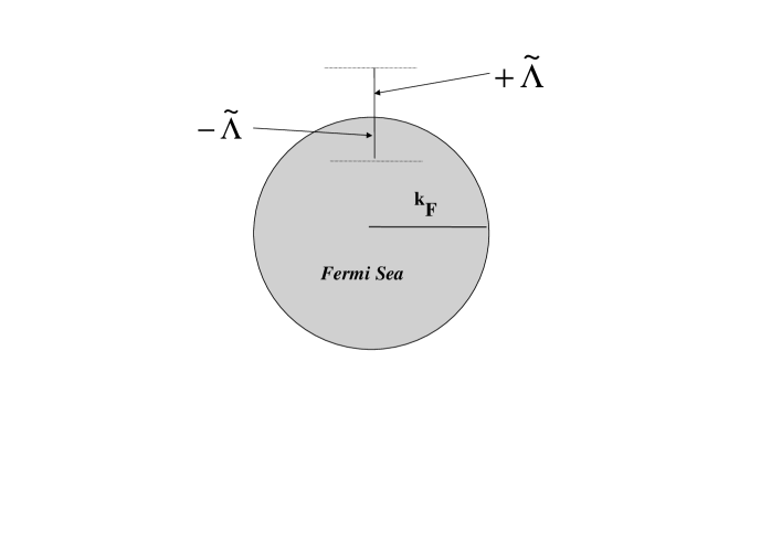
Figure 5: The decimation from $\tilde{\Lambda}$ on top of the Fermi sea down to the Fermi surface.

The $bare$ action that we will start with is supposed to be determined at $\tilde{\Lambda}$ and takes the form

$$S = S_{0}+S_{\pi}+S_{I},$$ (3.108)

$$S_{0} = \int dtd^{3}p\left[N^{\dagger}(p)i\partial_{t}N(p)-(\epsilon(p)-\epsilon_{F})N^{\dagger}(p)N(p)\right],$$

$$S_{I} = \int dt\int d^{3}p_{1}\cdots d^{3}p_{4}$$ (3.109)

$$\delta^{3}(\vec{p_{1}}+\vec{p_{2}}+\vec{p_{3}}+\vec{p_{4}})u(p_{1},p_{2},p_{3},p_{4})N^{\dagger}(p_{1})N(p_{2})N^{\dagger}(p_{3})N(p_{4})+\cdots$$

where $S_{\pi}$ is the well-known pionic action given entirely by chiral symmetry which I will not write down explicitly here. The four-Fermi vertex $u$ contains both local and non-local interactions, the former coming from integrating out the vector mesons and other heavy mesons and the latter coming from the pion exchange. When we localize the interactions, then the local part of the pion exchange will combine to the heavy meson part.

The objective of the calculation is to obtain the $S^{eff}$ of

$$Z = \int[d\Phi_{<}]e^{-S^{eff}(\Phi_{<})},$$ (3.110)

$$S^{eff}(\Phi_{<}) = \int^{\tilde{\Lambda}/s}_{-\tilde{\Lambda}/s}{\cal L}^{eff}(\Phi_{<}).$$ (3.111)

with $s>1$. The degrees of freedom integrated out, i.e., $\Phi_{>}$ is indicated in Fig. 6. The effective action $S^{eff}$ is to be computed in the manner described in the first part of my second lecture. I will describe what comes out in the next subsection.

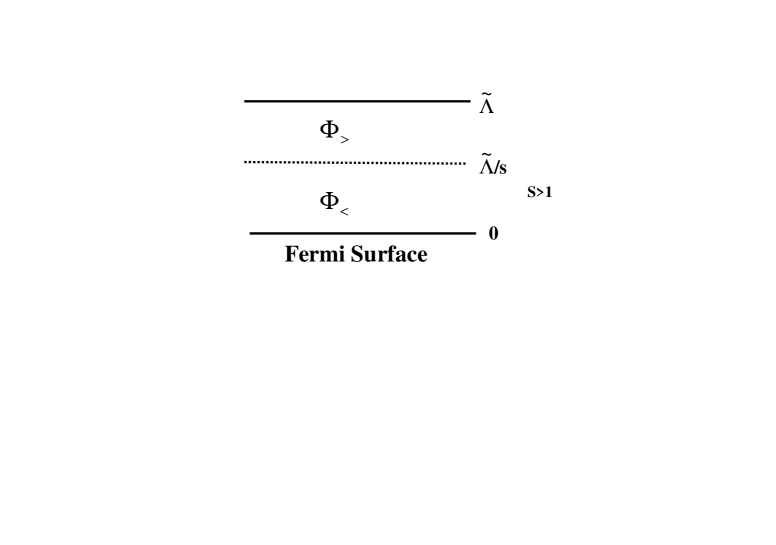
Figure 6: The decimation by integrating out $\Phi_{>}$ from $\tilde{\Lambda}$ to $\tilde{\Lambda}/s$ for $s>1$ on top of the Fermi.

The full decimation corresponds to sending $s$ to $\infty$.

5.2 Fermi-Liquid Fixed Points

By now we know what the standard procedure is. First we decide that $S_{0}$ remain marginal under the scaling. This means that the Fermi velocity $k_{F}/m^{\star}$ is marginal where $m^{\star}$ is the effective mass to be defined precisely below. We choose to fix the Fermi momentum $k_{F}$. This choice implies then that $m^{\star}$ should be a fixed-point quantity. This $m^{\star}$ is the Landau mass for the quasiparticle in Fermi-liquid theory. Next once we have the scaling law for the nucleon field by the rule that $S_{0}$ be marginal and $m^{\star}$ be at a fixed point, then we find that for the component of $u$ that does not scale, i.e., goes as a constant, the four-Fermi interaction $S_{I}$ is marginal for (1) the BCS channel denoted by $V$, (2) the ZS (zero sound) denoted by ${\cal F}$ and (3) the ZS^′ denoted by $\bar{{\cal F}}$ as pictured in Fig. 7. The quaisparticles interacting through the four-Fermi vertex are sitting on the Fermi surface, i.e., $|\vec{p_{i}}|=k_{F}$ with only the angular variables varying. (For simplicity, I am using the kinematics in 2 space dimensions in Fig. 7. The kinematics are similar in 3 space dimensions, just more complicated.) A constant $u$ is a local vertex and it will contain then local interactions coming from heavy-meson exchanges as well as the contact interaction in the pion exchange. Higher-order terms in momentum transfer that arise in localizing the non-local terms will be “irrelevant” and hence do not contribute in the decimation.

Figure 7: Tree and one-loop graphs for the BCS channel $\hat{\Omega}_{1}+\hat{\Omega}_{2}=\hat{\Omega}_{3}+\hat{\Omega}_{4}=0$, the ZS channel $\hat{\Omega}_{1}=\hat{\Omega}_{3},\hat{\Omega}_{2}=\hat{\Omega}_{4}$ and ZS^′ channel $\hat{\Omega}_{2}=\hat{\Omega}_{3},\hat{\Omega}_{1}=\hat{\Omega}_{4}$ where $\hat{\Omega}$ is the unit vector in 2 dimensions $\hat{\Omega}=\vec{p}/|\vec{p}|$. Note that $|\vec{p}_{i}|=k_{F}$.

Now given the marginal terms, one needs to compute the loop graphs in the decimation procedure. How this is done is explained in detail in the reviews and lecture notes, e.g., [SHANK, POL, CFROS]. Let me summarize:

• The BCS channel:

  The tree term is marginal as mentioned above. One-loop as well as higher-order graphs are non-vanishing and contribute to the renormaliztion group equation for the interaction. Summing the graphs to all orders, one finds

  $$V\sim\frac{v}{1+cv\ln s}$$ (3.112)

  where $v$ is the constant interaction coming from the $u$ vertex in the BCS channel and $c$ is a positive constant. If $v$ is repulsive, $v>0$, then nothing interesting happens and as $s$ goes to $\infty$ in decimation, the interaction dwindles away. However if the interaction is attractive, $v<0$, then there is a Landau pole and the system becomes unstable. This is the BCS phenomenon, leading to superconductivity if charged and to superfluidity if uncharged. This is the phenomenon that takes place at the superhigh density considered above when the color-flavor locking takes place, giving rise to color superconductivity.

• The ZS channel:

  It is easy to show that the loop terms vanish identically to all orders. This means a fixed point

  $$\frac{d{\cal F}}{d\ln s}=0.$$ (3.113)

• The ZS^′ channel:

  Here the loop correction to the RGE goes like $\sim\frac{d\tilde{\Lambda}}{k_{F}}\rightarrow 0$ for a given $k_{F}$ where $k_{F}$ is the Fermi momentum. This can be shown to be the case to all orders of loop corrections. The argument here is like $1/N$ expansion with $\frac{k_{F}}{d\tilde{\Lambda}}$ playing the role of $N$. Thus

  $$\frac{d\bar{{\cal F}}}{d\ln s}=0.$$ (3.114)

To summarize, nuclear matter can be described by an EFT with a Fermi surface with two fixed point quantities, the effective mass of the quasiparticle $m^{\star}$ called “Landau effective mass” and the interaction ${\cal F}$ called “Landau quasiparticle interaction”. What is essential in this EFT description is that one holds fixed the Fermi momentum $k_{F}$ which is equivalent to fixing density. This means that for a given density, one has the sets of Landau parameters that remain invariant under the renormalization group flow.

5.3 “Intrinsic Density Dependence” and Landau Parameters

In Lecture III, we learned that the HLS theory matched to QCD at the matching scale $\bar{\Lambda}$ in dense medium has a set of parameters that have intrinsic density dependence that is not accessible to perturbative calculation. Such a theory, when probed at a given density $n\sim n_{0}$ ($n_{0}$ is nuclear matter density), will then possess density dependent masses and coupling constants. We have just learned above that the Landau fixed point parameters are also given for given densities, that is, density-dependent. The question I want to pose here is: Is there any connection between the two?

I do not have the clear answer to this intriguing question but let me describe the initial effort in this direction and see how far we can go. What we will do here is to construct a model that possesses correct symmetries (e.g., chiral symmetry etc.) and density dependence that describes the ground state of nuclear matter and then fluctuate around that ground state to compute interesting response functions.

5.3.1 Walecka mean field theory with intrinsic density dependence

Let us consider that $\Phi_{L}$ now contains nucleons, pions and vector mesons. In fact the same can be formulated with the vector mesons and other heavy mesons integrated out but it is convenient to put the vectors and a scalar meson denoted $\phi$ explicitly. In free space this scalar may be the scalar meson with a broad width which is being hotly debated nowadays. For the symmetric nuclear matter for which we will apply mean field approximation, we can drop the pions and the $\rho$ mesons. The Lagrangian we will consider is

$${\cal L}=\bar{N}(i\gamma_{\mu}(\partial^{\mu}+ig^{\star}\omega^{\mu})-M^{\star}+h^{\star}\phi)N-\frac{1}{4}F^{2}_{\mu\nu}+\frac{1}{2}{m^{\star}_{\omega}}^{2}\omega^{2}+\frac{1}{2}(\partial_{\mu}\phi)^{2}-\frac{1}{2}{m^{\star}_{\phi}}^{2}\phi^{2}.$$ (3.115)

Apart from the stars appearing in the parameters, this is of the same form as Walecka’s linear mean field model [SEROT]. I should emphasize that this Lagrangian can be made consistent with chiral symmetry by restoring pion fields and identifying $\phi$ as a chiral scalar, not as the fourth component of the chiral four vector as in linear sigma model. The $\omega$ meson is a chiral scalar.

Suppose now that we do the mean field approximation in computing nuclear matter properties. If one simply puts the density dependence as $m^{\star}=m(n)$, $n$ being the matter density, and do the mean field, one does not get the right answer. In fact, one loses the conservation of energy-momentum tensor and thermodynamics does not come out right as a consequence. This has been a long standing difficulty in naively putting density dependence into the parameters of a mean field theory Lagrangian.

There may be more than one resolutions to this problem. One such solution was found by Song, Min and Rho [SMR,SONG]. The idea is to make the parameters of the Lagrangian a chiral invariant functional of the density field $operator$ $\check{n}$ defined by

$$\check{n}u^{\mu}=\bar{N}\gamma^{\mu}N$$ (3.116)

with unit fluid 4-velocity

$$u^{\mu}=\frac{1}{\sqrt{1-\vec{v}^{2}}}(1,\vec{v})=\frac{1}{\sqrt{n^{2}-\vec{j}^{2}}}(n,\vec{j}).$$ (3.117)

Here $\vec{j}=\langle\bar{N}\vec{\gamma}N\rangle$ is the baryon current density and $n\equiv\langle N^{\dagger}N\rangle$ is the baryon number density. In mean field, the field dependence brings additional terms in the baryon equation of motion whereas it does not affect the meson equations of motion. These additional terms contribute to the energy momentum tensor a term of the form

$$\delta T^{\mu\nu}=-2\check{\Sigma}\bar{N}\gamma_{\mu}n^{\mu}Ng^{\mu\nu}$$ (3.118)

where

$$\check{\Sigma}=\frac{\partial{\cal L}}{\partial\check{n}}$$ (3.119)

which comes into the energy density and the pressure of the system. In many-body theory language, this additional term at mean field order corresponds to “rearrangement” terms. This simple manipulation restores all the conservation laws lost when a c-number density is used. The resulting energy density etc. is of the same form as that of linear Walecka model except that the mass and coupling constants are a function of density. Let me just use the scaling consistent with the BR scaling

$$\frac{m_{\omega}^{\star}}{m_{\omega}}\approx\frac{m_{\phi}^{\star}}{m_{\phi}}\approx\frac{M^{\star}}{M}=\Phi(n)$$ (3.120)

and

$$\frac{g^{\star}}{g}\approx\Phi(n)$$ (3.121)

with a universal scaling factor

$$\Phi(n)=\frac{1}{1+0.28n/n_{0}}.$$ (3.122)

The numerical value 0.28 in the denominator of $\Phi$ will be seen coming from nuclear gyromagnetic ratio in lead nuclei. Using the standard value for the masses for the $\omega$ and the nucleon and $m_{\phi}\approx 700$ MeV, I get the binding energy $BE=16.0$ MeV, the equilibrium density $k_{eq}=257.3$ MeV, $m^{\star}/M=0.62$ and the compression modulus $K=296$ MeV. These results agree well with experiments, much better than the simple Walecka linear model, in particular for the compression modulus. In fact they are comparable to the “best-fit” mean field model [FURNST] which gives $BE=16.0\pm 0.1$ MeV, $k_{eq}=256\pm 2$ MeV, $m^{\star}/M=0.61\pm 0.03$ and $K=250\pm 50$ MeV.

The use of the bilinear nucleon field operator (3.116) makes evident and direct the dependence on density of the parameters of the Lagrangian in the mean field approximation. One could perhaps use other field variables such as the scalar field $\phi$ which is chiral scalar. However the scalar field would affect only the equation of motion of the scalar field, not that of the fermion field. It would make the density dependence complicated since the ground-state expectation value (GEV) of the scalar field is only indirectly related to the number density. Also doing the mean field with the scalar would involve different approximations. This is an interesting possibility to explore, however; it has not yet been studied.

One more point to note. Use of the scaling relations (3.120) and (3.121) is an additional ingredient to the notion that there should be an intrinsic dependence on density in the parameters of the Lagrangian. It is not dictated by the RGEs and the QCD-HLS matching.

5.3.2 Response functions of a quasiparticle

Given the ground state as described above, we now would like to calculate the response to an external field of a quasiparticle sitting on top of the Fermi sea. Here I will discuss response to the electromagnetic (EM) field. The response to the weak field in the axial channel is not yet well understood.

Consider a (non-relativistic) quasiparticle sitting on top of the Fermi sea with the momentum $\vec{p}$ which is probed by a slowly varying EM field. The convection current is given by

$$\vec{J}=g_{l}\frac{\vec{p}}{M}$$ (3.123)

with $|\vec{p}|\approx k_{F}$, where $M$ is the free-space nucleon mass and $g_{l}$ is the orbital gyromagnetic ratio given by

$$g_{l}=\frac{1+\tau_{3}}{2}+\delta g_{l}.$$ (3.124)

It is important to note that it is the free-space mass $M$, not an effective mass $m^{\star}$, that appears in (3.123). This is so because of the charge conservation or more generally gauge invariance. In condensed matter physics, such a requirement is known for the cyclotron frequency of an electron in magnetic field as “Kohn theorem.”

To calculate $g_{l}$, one starts with a chiral Lagrangian with the parameters of the Lagrangian density-dependent as determined by the mean field property as described in the last subsection and then calculates fluctuations on top of the ground state. This has been discussed extensively in the literature [FRS:98, RHO:MIG, BR:PR01], so I shall not go into details. The calculation is rather straightforward and the result is

$$\delta g_{l}=\frac{4}{9}\left[\Phi^{-1}-1-\frac{1}{2}\tilde{F}^{\pi}_{1}\right]\tau_{3}$$ (3.125)

where $\tilde{F}^{\pi}_{1}$ is the $l=1$ component of the Landau parameter $F$ – the spin- and isospin-independent component of the quasiparticle interaction ${\cal F}$ – coming from one-pion exchange which is of course given unambiguously by the chiral Lagrangian for a given $k_{F}$. The expression is valid for density up to $\sim n_{0}$ but cannot be pushed to the regime where $\Phi\ll 1$. (When $\Phi\ll 1$, then the nucleon cannot be treated non-relativistically and hence (3.125) will break down.)

For nuclear matter density,

$$\tilde{F}^{\pi}_{1}(n_{0})=-0.153$$ (3.126)

and from an experiment for a proton in the lead region

$$\delta g_{l}^{p}=0.23\pm 0.03.$$ (3.127)

This then gives

$$\Phi(n_{0})\approx 0.78.$$ (3.128)

In terms of the parameterization $\Phi(n)=(1+yn/n_{0})^{-1}$, this corresponds to $y=0.28$ used before for the ground state of nuclear matter.

Other applications of the relation are discussed in the references given above. What we have gotten here is a beginning of the relation between the hadronic parameters effective in medium of an effective Lagrangian matched to QCD and many-body interactions characterized by a number of fixed points around the Fermi surface. Much work needs to be done to unravel the intricate connections that we have a glimpse of.

6 Comments on the Literature

I summarize the main references I used for my lectures. They will be incomplete, since I focus mainly only on issues I have been working on recently. I will be leaving out many of the important papers in the field for which my apologies. $\bullet$ Lecture I:

The idea of Cheshire Cat was first introduced formally by Nadkarni, Nielsen and Zahed [41] and phenomenologically by Brown, Jackson, Rho and Vento [4]. The subsequent developments are summarized in [55, 43] on which my discussions are based. Some of the similar topics are reviewed by Hosaka and Toki [23]. The resolution of “proton spin problem” in the context of Cheshire Cat is described in [36, 20].

$\bullet$ Lecture II: Dilute matter:

An early attempt to incorporate Weinberg’s counting rule [67] into nuclear chiral effective field theory was made in 1982 [53] . It was incomplete, however, and it was only after Weinberg’s 1990 paper on the counting rule in pion-nuclear interactions that what was missing in 1982 was restored [56]. Applying Weinberg’s counting rule to nuclear force was made by Ordó$\tilde{\rm n}$ez and van Kolck [44]. Since then, many papers have been published in which counting schemes different from that of Weinberg have been investigated. These developments are extensively summarized in [3]. The importance of conformal invariant fixed point in nuclear physics was pointed out by Mehen, Stewart and Wise [39]. That the Weinberg counting rule would not be invalidated if one were to do a regularization appropriate to EFT in the Wilsonian sense (i.e., the role of power divergences in EFT) was argued in [45]. There have been published a large number of papers that improve on the construction of two-nucleon as well as multi-nucleon forces to high orders in chiral perturbation theory. The most recent efforts are summarized in [13, 14].

In [47], the thesis was put forward that the power of EFT in nuclear physics lies in making predictions for processes that are important for other areas of physics (such as astrophysics) but can be provided neither by the standard nuclear physics approach alone nor by the straightforward low-order power counting approach. This point was illustrated in the precise calculation of the solar $pp$ process [50] and $hep$ process [51]. In doing these calculations, it was argued that incorporating accurate nuclear wave functions obtained in the SNPA into the framework of EFT as an integral part of EFT is both justified and more effective  than the approach based on SNPA alone or on strict adherence to counting rules.

$\bullet$ Lecture II: Superdense matter

The literature on this topic is huge. Since color superconductivity per se is not the main focus of this part of lecture, I use only the review by Rajagopal and Wilczek [57]. One can find an extensive list of references in this review. The EQCD (effective QCD) Lagrangian obtained at high density by decimating toward the Fermi surface was first made (as far as I know) by Hong [21]. The first formulation as an EFT of the collective modes that arise in the color-flavor locking was made simultaneously by Hong, Rho and Zahed [24] (hep-ph/9903503) and by Casalbuoni and Gatto [11] (hep-ph/9908227). It was argued in [24] that solitons in the effective chiral Lagrangian in the CFL phase, called “qualitons,” could be identified as baryons in the system. It was realized then that the EFT Lagrangian with the gluons included is of the HLS form and that bound-state excitations of diquarks could arise in the super-pion and super-vector-meson channels [RWZ]. These could be coupled to the Golstone bosons and Higgsed vector mesons in a way analogous to the “sobar” description [KRBR]. The “quark-hadron continuity” conjecture was put forward by Schäfer and Wilczek [65].

$\bullet$ Lecture III:

The idea that the color-flavor locking “observed” at superhigh density can also take place at zero density was presented by Wetterich in a series of papers [70] soon after the CFL was proposed at high density. That Wetterich’s CFL scenario – which is a “top-down” approach – coincides with Harada-Yamawaki’s HLS scenario – which is a “bottom-up” approach – was noticed in [5, 7]. The discovery of vector manifestation in chiral symmetry by Harada and Yamawaki [30, 27, 28, 29] led to a series of new developments discussed in the lecture, namely the vanishing of the vector meson mass at the chiral transition [26, 25, 22] and the derivation of one of BR scalings. The interplay of Wetterich’s approach and Harada-Yamawaki’s approach suggests an equivalence of explicit and hidden gauge symmetries, somewhat analogous to Weinberg’s observation [68] on non-uniqueness in going from one to the other between non-gauge-symmetric effective field theory and gauge symmetric theory.

$\bullet$ Lecture IV:

The notion that Landau Fermi liquid theory is a bona-fide EFT has been advocated and developed by, among others, Shankar [61], Polchinski [52] and Frölich et al [10]. That Walecka theory of nuclear matter is equivalent to Landau-Migdal Fermi liquid theory was shown sometime ago by Matsui [38]. By relating BR scaling to Fermi-liquid fixed point parameters, the authors in [15, 16, 62, 64] constructed an effective field theory for nuclear matter in terms of BR scaling parameters. This mapping of chiral Lagrangian field theory to Fermi-liquid fixed point theory has met with success in explaining the anomalous gyromagnetic ratio in heavy nuclei [16] but has not been satisfactorily tested in weak axial transitions other than axial-charge transitions. How to incorporate axial responses in the framework of Landau theory and effective chiral Lagrangian is not yet worked out. The present status in this direction is summarized in [54].

Arriving at nuclear matter starting with chiral Lagrangians defined in matter-free space was initiated seriously by Lynn [37]. Recent works focusing on chiral perturbation theory in medium posit the presence of a Fermi sea and develop perturbations around the Fermi surface [33].

Acknowledgments

I have benefitted from recent discussions and/or collaborations with Gerry Brown, Masayasu Harada, Youngman Kim, Vicente Vento and Koichi Yamawaki. Giving these lectures at the spectacularly beautiful mountain region Hualien, Taiwan was a real pleasure. I would like to thank the organizers, in particular Shin Nan Yang and Wen-Chen Chang, of the Spring School for the opportunity. Some of these lectures were prepared when I was visiting KIAS in the Autumn 2001 and I would like to acknowledge the Institute’s hospitality.

References

- [1]
- [2] [BANDO] M. Bando, T. Kugo and K. Yamawaki, Phys. Rep. 164 (1988) 217.
- [3] [BEANE] S.R. Beane, P.F. Bedaque, W.C. Haxton, D.R. Phillips and M.J. Savage, “From hadrons to nuclei: Crossing the border,” nucl-th/0008064.
- [4] [BJRV] G.E. Brown, A.D. Jackson, M. Rho and V. Vento, Phys. Lett. B140 (1984) 285.
- [5] [BR:BERK] G.E. Brown and M. Rho, AIP Proceedings (2001 Nuclear Physics Conference, Berekely, California, August, 2001), nucl-th/0108050
- [6] [BR:PRL] G.E. Brown and M. Rho, Phys. Rev. Lett. 66 (1991) 2720.
- [7] [BR:PR01] G.E. Brown and M. Rho, Phys. Rep. (2002), hep-ph/0103102.
- [8] [BR:PR96] G.E. Brown and M. Rho, Phys. Rep. 269 (1996) 333.
- [9] [CHAP] G. Chapline, E. Hohlfeld, R.B. Laughlin and D.I. Santiago, “Quantum phase transitions and the breakdown of classical general relativity,” gr-qc/012094.
- [10] [CFROS] T. Chen, J. Fröhlich, and M. Seifert, “Renormalization group methods: Landau Fermi liquid and BCS superconductors,” lectures at Les Houches summer school, August 1994, cond-mat/9508063
- [11] [CG] R. Casalbuoni and R. Gatto, Phys. Lett. B464 (1999) 111.
- [12] [CR:71] M. Chemtob and M. Rho, Nucl. Phys. A163 (1971) 1.
- [13] [EPEL1] E. Epelbaum, U.-G. Meissner, W. Göckle and Ch. Elster, nucl-th/0106007.
- [14] [EPEL2] E. Epelbaum, A. Nogga, W. Glöckle, H. Kamada, U.-G. Meissner and H. Witala, nucl-th/0201064
- [15] [FR:96] B. Friman and M. Rho, Nucl. Phys. A606 (1996) 303.
- [16] [FRS:98] B. Friman, M. Rho and C. Song, Phys. Rev. C59 (1999) 3357.
- [17] [FURNST] R.J. Furnstahl and B. Serot, Nucl. Phys. A671 (2000) 447.
- [18] [GASS] J. Gasser and H. Leutwyler, Ann. Phys. (NY) 158 (1984) 142; Nucl. Phys. B250 (1985) 465.
- [19] [GEORGI] H. Georgi, Phys. Rev. Lett. 63 (1989) 1917; Nucl. Phys. B331 (1990) 311.
- [20] [HJL] H.-J. Lee, Seoul National University thesis (2001), unpublished.
- [21] [HONG] D.K. Hong, Phys. Lett. B473 (2000) 118; Nucl. Phys. B582 (2000) 451; hep-ph/0101025.
- [22] [HKR] M. Harada, Y. Kim and M. Rho, Phys. Rev., hep-ph/0111120.
- [23] [HOSAKA] A. Hosaka and H. Toki, Phys. Rep. 277 (1996) 65.
- [24] [HRZ] D.K. Hong, M. Rho and I. Zahed, Phys. Lett. B468 (1999) 261.
- [25] [HS:T] M. Harada and C. Sasaki, “Vector manifestation in hot matter,” hep-ph/0109034
- [26] [HY:CONF] M. Harada and K. Yamawaki, Phys. Rev. Lett. 83 (1999) 3374.
- [27] [HY:FATE] M. Harada and K. Yamawaki, Phys. Rev. Lett. 87 (2001) 152001.
- [28] [HY:MATCH] M. Harada and K. Yamawaki, Phys. Rev. D64 (2001) 014023.
- [29] [HY:PR] M. Harada and K. Yamawaki, Phys. Rep., in preparation.
- [30] [HY:VM] M. Harada and K. Yamawaki, Phys. Rev. Lett. 86 (2001) 757, hep-ph/0010207.
- [31] [JOKA] D. Jido, M. Oka and A. Hosaka, Prog. Theor. Phys. 106 (2001) 873.
- [32] [KDR] K. Kubodera, J. Delorme and M. Rho, Phys. Rev. Lett. 40 (1978) 755.
- [33] [KFW] N. Kaiser, S. Fritsch and W. Weise, Nucl. Phys. A697 (2002) 255; Nucl. Phys. A700 (2002) 343.
- [34] [KR:91] K. Kubodera and M. Rho, Phys. Rev. Lett. 67 (1991) 3479.
- [35] [KRBR] Y. Kim, R. Rapp, G.E. Brown and M. Rho, Phys. Rev. C62 (2000) 015202.
- [36] [LMPRV] H.-J. Lee, D.-P. Min, M. Rho and V. Vento, Nucl. Phys. A657 (1999) 75.
- [37] [LYNN] B.W. Lynn, Nucl. Phys. B402 (1993) 281.
- [38] [MATSUI] T. Matsui, Nucl. Phys. A370 (1981) 365.
- [39] [MEHEN] T. Mehen, I.W. Stewart and M. Wise, Phys. Lett. B474 (2000) 145.
- [40] [MK] P.D. Morley and M.B. Kislinger, Phys. Rep. 51 (1979) 63.
- [41] [NNZ:CC] S. Nadkarni, H.B. Nielsen and I. Zahed, Nucl. Phys. B253 (1984) 308.
- [42] [NRWZ] H.B. Nielsen, M. Rho, A. Wirzba and I. Zahed, Phys. Lett. B269 (1991) 389; Phys. Lett. B281 (1992) 345.
- [43] [NRZ] M.A. Nowak, M. Rho and I. Zahed, Chiral Nuclear Dynamics (World Scientific, Singapore, 1996).
- [44] [OVK] C. Ordóez and U. van Kolck, Phys. Lett. B291 (1992) 114; L. Ray, C. Ordóez and U. van Kolck, Phys. Rev. Lett. 72 (1994) 1982.
- [45] [PKMR:CO] T.-S. Park, K. Kubodera, D.-P. Min and M. Rho, Nucl. Phys. A646 (1999) 83.
- [46] [PKMR:M1/E2] T.-S. Park, K. Kubodera, D.-P. Min and M. Rho, Phys. Lett. B472 (2000) 232.
- [47] [PKMR:TAI] T.-S. Park, K. Kubodera, D.-P. Min and M. Rho, Nucl. Phys. A684 (2001) 101c.
- [48] [PMR] T.-S. Park, D.-P. Min and M. Rho, Phys. Rev. Lett. 74 (1995) 4153; Nucl. Phys. A596 (1996) 515
- [49] [PMRV] B.-Y. Park, D.-P. Min, M. Rho and V. Vento, nucl-th/0201014.
- [50] [PMSV:pp] T.-S. Park, L.E. Marcucci, R. Schiavilla, M. Viviani, A. Kievsky, S. Rosati, K. Kubodera, D.-P. Min and M. Rho, nucl-th/0106026.
- [51] [PMSV:hep] T.-S. Park, L.E. Marcucci, R. Schiavilla, M. Viviani, A. Kievsky, S. Rosati, K. Kubodera, D.-P. Min and M. Rho, nucl-th/0107012.
- [52] [POL] J. Polchinski, Recent Directions in Particle Theory: From Superstrings and Black Holes to the Standard Model, edited by J. Harvey and J. Polchinski (World Scientific, Singapore, 1994) p235-274
- [53] [RHO:ERICE] M. Rho, Prog. in Part. and Nucl. Phys. 8 (1982) 103.
- [54] [RHO:MIG] M. Rho, Yad. Fiz. (A.B. Migdal Memorial) 64 (2001) 696.
- [55] [RHO:PR] M. Rho, Phys. Rep. 240 (1994) 1.
- [56] [RHO:PRL] M. Rho, Phys. Rev. Lett. 66 (1991) 1275.
- [57] [RW] K. Rajagopal and F. Wilczek, hep-ph/0011333.
- [58] [RWZ] M. Rho, A. Wirzba abd I. Zahed, Phys. Lett.B473 (2000) 126.
- [59] [SCHWINDT] O. Schwindt and N.R. Walet, hep-ph/0201203.
- [60] [SEROT] B.D. Serot and J.D. Walecka, Adv. Nucl. Phys. 16 (1986) 1.
- [61] [SHANK] R. Shankar, Rev. Mod. Phys. 66 (1994) 129
- [62] [SMR] C. Song, D.-P. Min and M. Rho, Phys. Lett. B424 (1998) 226.
- [63] [SON] D.T. Son and M.A. Stephanov, Phys. Rev.D61 (2000) 074012.
- [64] [SONG] C. Song, Phys. Rep. 347 (2001) 289.
- [65] [SW:CONT] T. Schäfer and F. Wilczek, Phys. Rev. Lett. 82 (1999) 3956.
- [66] [VOLO] G.E. Volovik, Phys. Rep., to appear, gr-qc/0005091.
- [67] [WEIN:CHI] S. Weinberg, Physica (Amsterdam) 96A (1979) 327.
- [68] [WEIN:GAUGE] S. Weinberg, Phys. Rev. D56 (1997) 2303.
- [69] [WEIN:MEND] S. Weinberg, Phys. Rev. Lett. 65 (1990) 1177.
- [70] [WETT] C. Wetterich, Phys. Rev. D64 (2001) 036003; hep-ph/0011076; hep-ph/0102248; J. Berges and C. Wetterich, Phys. Lett. B512 (2001) 85, hep-ph/0012311; J. Berges, Phys. Rev. D64 (2001) 014010, hep-ph/0012013.