Nuclear magnetization distribution and hyperfine splitting in Bi⁸²⁺ ion

Abstract

Hyperfine splitting in Bi⁸²⁺ and Pb⁸¹⁺ ions was calculated using continuum RPA approach with effective residual forces. To fix the parameters of the theory the nuclear magnetic dipole moments of two one-particle and two one-hole nuclei around ²⁰⁸Pb were calculated using the same approach. The contribution from velocity dependent two-body spin-orbit residual interaction was calculated explicitly. Additionally, the octupole moment of ²⁰⁹Bi and the hfs in muonic bismuth atom were calculated as well in the same approach. All the calculated observables, except the electronic hfs in ²⁰⁹Bi, are in good agreement with the data. We argue for more accurate measurement of the octupole moment and the muonic hfs for ²⁰⁹Bi.

1 Introduction

High experimental precision attained in the laser spectroscopic measurement of the ground-state hfs in hydrogen-like ²⁰⁹Bi⁸²⁺ [1] stimulates considerable theoretical activity in this field (see, e.g., [11, 12, 13, 14, 15, 16, 17, 18, 19] and references therein).

$$\Delta E_{hfs}^{exper.}=\,5.0840(8)\,\mbox{eV}.$$ (1)

The first quantum mechanical calculation of the hfs was made by Fermi in $1930$ [2]. He treated the hfs with a non-relativistic formalism in studies of alkali atoms, where he derived approximate generalizations from the hydrogenic case. In the case of ²⁰⁹Bi⁸²⁺ the formulae obtained by Fermi give a value about $2.75$ eV, which is $46\%$ smaller than the experimental value (1). Relativity can be taken into account by multiplying non-relativistic value with a relativistic correction factor $A(\alpha Z)$ [3]. In bismuth case $Z=83$ and factor $A(\alpha Z)=2.125$. The relativistic generalization of the Fermi formulae holds for point-like nucleus and gives a hfs for ²⁰⁹Bi⁸²⁺ of about $5.84$ eV, which is $15\%$ larger than the experimental value (1).

The effect of spatial distribution of the nuclear charge was analyzed in pioneering works by Rosenthal, Breit [4] and others [5, 6] and it is sometimes called ”Breit-Rosenthal effect”. The correction factor for the nuclear charge distribution can be written as $(1-\delta)$, where $\delta$ is a small number which depends mainly on the root-mean-square (rms) radius of the nuclear charge distribution, $\left<r_{c}{}^{2}\right>^{1/2}$. By assuming a uniform spherical symmetric charge distribution and using the experimental value $\left<r_{c}{}^{2}\right>^{1/2}=\,5.519(4)$ fm [7] for the nuclear charge distribution, $\delta$ can be calculated to be $0.0110$ in the case of ²⁰⁹Bi⁸²⁺ [8]. The relativistic hfs energy splitting in ²⁰⁹Bi⁸²⁺ for a uniformly charged nucleus becomes than about $5.20$ eV, which is $2\%$ larger than the experimental value (1).

There are two principal corrections to the Fermi-Breit formulae that is necessary to take into account: the magnetic moment distribution within the nucleus [9, 10, 11, 12, 13, 14, 15] and radiative corrections [11, 16, 17, 18, 19]. Both of these corrections are of comparable magnitude.

The correction for an extended nuclear magnetization was first studied in an innovative work by A. Bohr and V. Weisskopf [9, 10] and is also called ”Bohr-Weisskopf effect”. Recently, three approaches for theoretical determination of the Bohr-Weisskopf effect have been used. The simplest of these approaches is based on a solution of the Schrödinger equation for a nucleon in a mean-field potential, the solution gives the distribution for the unpaired nucleon in the nucleus and the distribution is used to determine hyperfine splitting. This approach has been used by Shabaev et al. [11] and by Gustavsson et al. [12]. A slightly more sophisticated approach, giving equivalent results for the hfs in leading order, is the ”dynamical proton model” (DPM), where the odd proton of the bismuth nucleus is treated as a Dirac particle bound in a mean-field potential. The first order hfs in hydrogen-like Bi is then given by a photon exchange between the electron and the proton. DPM was introduced by Labzowsky et al. [13]. The third and more complete approach is a many-body calculation with the use of ”dynamical correlation model” (DCM). This approach is the only calculation of the Bohr-Weisskopf effect which includes many-body contributions and Tomaselli et al. have used it for studies of several systems [14, 15].

In addition to the dominant electrostatic and hyperfine interactions with nucleus, the electron also interacts with radiation field, an interaction described by QED. The leading QED corrections originate from the one-loop self-energy and vacuum-polarization effects. The one-loop QED effects for hfs have been calculated by different groups and the results are consistent [11, 16, 17, 18, 19].

In this work we consider a contribution of the magnetic moment distribution within the nucleus to the hydrogen-like ion hfs. Our approach is close to the one used in [20]. This microscopic approach is based mainly on the Migdal’s theory of finite Fermi system (FFST) [21] (see also [22, 23, 24]). Essentially, this approach is equivalent to calculation of the core polarization effects with the use of an effective interaction. The first calculation of the core polarization goes back to fifties [25] and this early development was summarized in [22]. Modern calculations, however, differ significantly in the size of the single-particle space included into sum over intermediate particle-hole states. For spherical nuclei all single-particle space, including continuum is included into calculation. This is one difference between our approach and the DCM where one has to use the restricted single-particle space. Another difference between our work and [14, 15] is that RPA accounts for ground state correlations represented graphically by backward going loops. And, finally, we use explicitly the correction to nuclear electromagnetic current due to velocity dependent interaction. This correction was absent in [14, 15] since they use velocity independent forces. Previously, this correction was discussed in [20] in connection to the Bohr-Weisskopf effect in bismuth muonic atom. It was shown that this correction is not negligible. Here we extend this analysis to the hydrogen-like ions around ²⁰⁸Pb nucleus.

2 Basic Equations

In FFST the effect of the core polarization is described by introducing an effective single-particle operator (vertex) $M$ satisfying the equation [21]

$$M(\omega)\,=\,e_{eff}\,M_{0}\,+\,F\,A(\omega)\,M(\omega),$$ (2)

where $M_{0}$ is in our case the bare single-particle $MJ$ operator, $A(\omega)$ the polarization operator of a particle-hole pair,

$$A^{(\omega)}_{\nu_{1}\,\nu_{2};\nu_{3}\,\nu_{4}}\,=\,\int\,\frac{d\varepsilon}{2\pi i}\,G_{\nu_{1}\,\nu_{3}}(\varepsilon+\frac{1}{2}\omega)\,G_{\nu_{2}\,\nu_{4}}(\varepsilon-\frac{1}{2}\omega),$$ (3)

where $G_{\nu\nu^{\prime}}(\varepsilon)$ is the single-particle Green function. $F$ is the amplitude of quasi-particle interaction. Equation (2) is written in the re-normalized form, i.e. after elimination of a regular part in the Green function $G_{\nu\nu^{\prime}}(\varepsilon)$. The regular part of the $G$-function corresponding to admixture of three- or more particle states produces the effective charges $e_{eff}$, and re-normalizes the interaction amplitude $F$ in (2). Following [21], we choose $e_{eff}$ as a constant independent of the particular state $\left|\nu\right>$, but different for the spin and orbital parts of the operator $M_{0}$:

$$e_{eff}\,M^{s}_{0}\,=\,\left\{\begin{array}[]{ll}(1-\zeta_{s})\,(M^{s}_{0})_{p}\,+\,\zeta_{s}\,(M^{s}_{0})_{n}\,,&\mbox{for protons,}\\ (1-\zeta_{s})\,(M^{s}_{0})_{n}\,+\,\zeta_{s}\,(M^{s}_{0})_{p}\,,&\mbox{for neutrons,}\\ \end{array}\right.$$ (6)

$$e_{eff}\,M^{l}_{0}\,=\,\left\{\begin{array}[]{ll}(1-\zeta_{l})\,(M^{l}_{0})_{p}\,,&\mbox{for protons,}\\ \zeta_{l}\,(M^{l}_{0})_{p}\,,&\mbox{for neutrons.}\\ \end{array}\right.$$ (9)

The constants $\zeta$ in (6) and (9) were taken as equal for both protons and neutrons since the main deviation of the magnetic moments from single-particle values is in the isovector part of the $MJ$ operator.

The effective interaction is $F=F_{ss}+F_{ls}$, where

$$F_{ss}\,=\,C\,(g+g^{\prime}\,\mbox{\boldmath{$\tau$}}_{1}\cdot\mbox{\boldmath{$\tau$}}_{2}\,)\,\mbox{\boldmath{$\sigma$}}_{1}\cdot\mbox{\boldmath{$\sigma$}}_{2}\,\delta(\mbox{${\bf r}$}_{1}-\mbox{${\bf r}$}_{2})$$ (10)

is the Migdal-type spin-spin zero-range interaction and

$$F_{ls}\,=\,C\,r_{0}^{2}\,(\kappa+{\kappa^{\prime}}\,\mbox{\boldmath{$\tau$}}_{1}\cdot\mbox{\boldmath{$\tau$}}_{2}\,)\cdot(\mbox{${\bf p}$}_{1}-\mbox{${\bf p}$}_{2})\cdot(\mbox{\boldmath{$\sigma$}}_{1}+\mbox{\boldmath{$\sigma$}}_{2})\times\nabla_{1}\delta(\mbox{${\bf r}$}_{1}-\mbox{${\bf r}$}_{2})$$ (11)

is the spin-orbit one.

The $MJ$ vertex $\mathcal{M}_{JM}$ can be written in coordinate representation in the form

$$\mathcal{M}_{JM}\,=\,\sum_{i=1}^{3}\,v{}^{i}(r)\,T^{(i)}_{JM},$$ (12)

where we have introduced the complete set of linear independent tensor operators

$$\begin{array}[]{c}T^{(1)}_{JM}\,=\,\mbox{\boldmath{$\sigma$}}\cdot{\bf Y}^{J-1}_{JM}({\bf n}),\;T^{(2)}_{JM}\,=\,\mbox{\boldmath{$\sigma$}}\cdot{\bf Y}^{J+1}_{JM}({\bf n}),\\ T^{(3)}_{JM}\,=\,\frac{1}{2}\left({\bf L}\cdot{\bf Y}^{J-1}_{JM}({\bf n})+{\bf Y}^{J-1}_{JM}({\bf n})\cdot{\bf L}\right),\end{array}$$ (13)

where ${\bf Y}^{L}_{JM}({\bf n})$ being the vector spherical harmonic [26].

The values of the $MJ$ moments can be expressed in terms of matrix elements of the vertex (12):

$$\mu_{J}\,=\,\left<\nu m=I\right|\mathcal{M}_{J0}(\omega=0)\left|\nu m=I\right>\,=\,\left(\begin{array}[]{ccc}I&J&I\\ -I&0&I\end{array}\right)\,\sum_{i=1}^{3}\,\left<nlI\right|v{}^{i}(r)\left|nlI\right>\,t^{(i)}_{\nu\nu},$$ (16)

where $\nu=(nlIm)$ is the set of nucleon quantum numbers, and $t^{(i)}_{\nu_{2}\nu_{1}}\,=\,\left(l_{2}I_{2}\|T^{(i)}_{J}\|l_{1}I_{1}\right)$ is the reduced matrix element of the tensor operators (13).

Reducing the angular and spin variables in equation (2) we obtain in coordinate representation the system of integrals equations

$$w{}^{i}(r)\,=\,e_{eff}\,w_{0}{}^{i}(r)\,+\,\sum_{j=1}^{3}\int_{0}^{\infty}dr^{\prime}\Theta^{ij}(r,r^{\prime}|\omega)\,w{}^{j}(r^{\prime}),$$ (17)

where we have introduce $w{}^{i}(r)\,=\,rv{}^{i}(r)$. The kernel of the integrals equations (17) is the sum of two terms

$$\Theta^{ij}\,=\,\Theta^{ij}_{ss}\,+\,\Theta^{ij}_{ls}.$$ (18)

For the spin-spin interaction (10)

$$\Theta^{ij}_{ss}\,=\,C\hat{g}\,\,rA^{ij}_{J}(r,r^{\prime}|\omega)r^{\prime},$$ (19)

where $\hat{g}\,=\,g+{g^{\prime}}\,\mbox{\boldmath{$\tau$}}_{1}\cdot\mbox{\boldmath{$\tau$}}_{2}\,$ and the sun over isospin variables is assumed. The polarization operator $A^{ij}_{J}(r,r^{\prime}|\omega)$ can be calculated in terms of the Green function $G_{lj}(r,r^{\prime}|\varepsilon)$ of the radial Schrödinger equation:

$$A^{ij}_{J}(r,r^{\prime}|\omega)\,=\,\frac{1}{2J+1}\sum_{j_{1}j_{2}l_{1}l_{2}}\,t^{(i)}_{\nu_{1}\nu_{2}}t^{(j)}_{\nu_{1}\nu_{2}}\,\sum_{n1}k_{\nu_{1}}R_{\nu_{1}}(r)R_{\nu_{2}}(r^{\prime})$$

$$\times\left[G_{l_{2}j_{2}}(r,r^{\prime}|\varepsilon_{\nu_{1}}-\omega)+G_{l_{2}j_{2}}(r,r^{\prime}|\varepsilon_{\nu_{1}}+\omega)\right],$$ (20)

where $k_{\nu}$ is the occupation number of the level $\nu=(nljm)$, and $R_{\nu}(r)$ is the single-particle radial wave function. The Green function can be calculated using two linear independent solution of the radial Schrödinger equation. This method allows one to use all of the single-particle spectrum [23],[24]. For the spin-orbit interaction (11) expression $\Theta^{ij}_{ls}$ in terms of $A^{ij}_{J}$ is more complicated (see [20]).

3 Hyperfine Splitting and Static MJ-moments

The ground-state hyperfine splitting of hydrogen-like ions is conveniently written in the form [11], [14]

$$\Delta E_{hfs}\,=\,\frac{4}{3}\alpha(\alpha Z)^{3}\frac{\mu}{\mu_{N}}\frac{m_{e}}{m_{p}}\frac{2I+1}{2I}\,m_{e}c^{2}\,A(\alpha Z)(1-\delta)(1-\varepsilon)+\Delta E_{QED}.$$ (21)

Here $\alpha$ is the fine-structure constant, $Z$ is the nuclear charge, $m_{e}$ is the electron mass, $m_{p}$ is the proton mass, $\mu$ is the nuclear magnetic moment, $\mu_{N}$ is the nuclear magneton, and $I$ is the nuclear spin. $A(\alpha Z)$ denotes the relativistic factor [3]

$$A(\alpha Z)\,=\,\frac{1}{\gamma(2\gamma-1)},\;\mbox{where}\;\gamma\,=\,\sqrt{1-(\alpha Z)^{2}}.$$ (22)

$\delta$ is the nuclear charge distribution correction, $\varepsilon$ is the nuclear magnetization distribution correction (the Bohr-Weisskopf correction) [9], and $\Delta E_{QED}$ is the QED correction. To obtain the first part of Eq. (21), one can start from the magnetic interaction of an electron and a nucleus

$$H_{int}\,=\,-\frac{1}{c^{2}}\int d^{3}rd^{3}r^{\prime}\frac{{\bf j}({\bf r})\cdot{\bf J}({\bf r^{\prime}})}{|\bf r-\bf r^{\prime}|},$$ (23)

where ${\bf j}({\bf r})$ and ${\bf J}({\bf r^{\prime}})$ are the electromagnetic current densities. The hfs can be written as

$$\Delta E_{hfs}\,=\,\Delta E_{1}+\Delta E_{QED},$$ (24)

where $\Delta E_{1}$ is the diagonal matrix element of 0-th spherical component of the vector vertex $\Gamma_{1\mu}({\bf r})$,

$$\Delta E_{1}\,=\,\left<\nu m=I|\Gamma_{10}|\nu m=I\right>.$$ (25)

The vertex $\Gamma_{1\mu}$ is the solution of equation (2) with the bare vertex $\Gamma^{0}_{1\mu}$ derived from (23),

$$\Gamma^{0}_{1\mu}\,=\,\frac{4eK}{j+1}\,\frac{2I+1}{2I}\,\left\{\mathcal{M}^{0}_{1\mu}\Omega^{(0)}_{nlj}-\sqrt{4\pi}\,\mu_{N}\sum_{a}\,\left[g_{s}(a)\,T^{(1)}_{1\mu}(a)+g_{l}(a)\,T^{(3)}_{1\mu}(a)\right]\,\Omega^{(1)}_{nlJ}(r_{a})\,\right.$$

$$\left.+\sqrt{4\pi}\,\mu_{N}\sum_{a}\,\left[g_{l}(a)\,T^{(3)}_{1\mu}(a)\right.-\sqrt{\frac{1}{2}}\left.g_{s}(a)\,T^{(2)}_{1\mu}(a)\right]\,\Omega^{(2)}_{nlJ}(r_{a})\right\}.$$ (26)

In this expression the sum is taken over the nucleons, $K=(l-j)(2j+1)$ for the atomic states with $j=l\pm\frac{1}{2}$,

$$\Omega^{(0)}_{nlj}\,=\,\int_{0}^{\infty}dr^{\prime}f_{nlj}(r^{\prime})g_{nlj}(r^{\prime}),$$ (27)

$$\Omega^{(1)}_{nlj}(r)\,=\,\int_{0}^{r}dr^{\prime}f_{nlj}(r^{\prime})g_{nlj}(r^{\prime}),$$ (28)

$$\Omega^{(2)}_{nlj}(r)\,=\,\frac{1}{r^{3}}\,{\int}^{r}_{0}dr^{\prime}{r^{\prime}}^{3}f_{nlj}(r^{\prime})g_{nlj}(r^{\prime}),$$ (29)

where $f_{nlj}(r)$ and $g_{nlj}(r)$ are the upper and the lower components of the Dirac radial wave function. The vertex $\mathcal{M}^{0}_{1\mu}$ is the bare operator of the nuclear magnetic dipole moment. The bare operator of the nuclear magnetic multipole moments has a standard form [27]

$$\mathcal{M}^{0}_{JM}\,=\,\sqrt{4\pi J}\mu_{N}\sum_{a}\,r_{a}^{J-1}\,\left(g_{s}(a)\,T^{(1)}_{JM}(a)+g_{l}(a)\,\frac{2}{J+1}T^{(3)}_{JM}(a)\right).$$ (30)

The vertex $\Gamma^{0}_{1\mu}$ is $M1$ part of the interaction (23) averaged over atomic state with the quantum numbers $n$,$l$,$j$. Higher moments of the interaction (23) do not contribute to hfs for the electron ground state with $j=1/2$.

The same equations (2) can be used to calculate nuclear magnetic multipole moments $\mathcal{M}_{JM}$ with the bare vertex (30). The Eqs. (3), (30) obtained using the standard electromagnetic current density for free nucleons. However, due to velocity dependence of the spin-orbit interaction (11), there are the corrections to electromagnetic current density. The corrections were discussed earlier [27, 20]. They produce an additional contributions to the bare vertexes $\mathcal{M}^{0}_{JM}$ and $\Gamma^{0}_{1\mu}$ and can be presented in the similar form as (3),(30). The corresponding equations can be found in the Appendix A.

It is worth to note, that the expression for hfs (3) is a sum of three terms. The first, being proportional $\Omega^{(0)}_{nlj}$, corresponds to a point-like magnetic moment distribution. It does not contribute to the correction $\epsilon$. This term gives the main contribution to hfs being larger than two other terms by about two orders of magnitude. The effects of nuclear structure are not essential here, they are hidden in the value of the nuclear magnetic moment which is well known from the experiment. Two other terms are, just, the correction for an extended nuclear magnetization. But, only the second term is proportional to the magnetic moment density, while the third one is not.

The kernel (18) of the Eq.(17) was calculated using partially self-consistent mean field potential [28]. The potential includes four terms. The isoscalar term is the standard Woods-Saxon potential

$$U_{0}(r)=-\frac{V}{1+\exp{\frac{r-R}{a}}},$$ (31)

with the parameters $V=52.03$ MeV, $R=1.2709A^{1/3}$ fm, and $a=0.742$ fm [28]. Two other terms $U_{ls}(r)$, and $U_{\tau}(r)$ were calculated self-consistently using two-body interaction Eq.(11) for the spin- orbit part of the potential, and the Migdal-type isovector interaction

$$F_{\tau}=f^{\prime}C(\mbox{\boldmath$\tau$}_{1}\cdot\mbox{\boldmath$\tau$}_{2})\delta({\bf r}_{1}-{\bf r}_{2})$$ (32)

for the isovector part of the potential, with $f^{\prime}=1.075$ [28]. The last term is the Coulomb interaction that was calculated for uniform charge sphere distribution with $R_{C}=1.18A^{1/3}$. This potential produces for ²⁰⁹Bi nucleus a charge density with rms. $\left<r_{c}{}^{2}\right>^{1/2}=5.52$ fm, which is in fair agreement with the measured value 5.519(4) fm [7].

The parameters of the interactions Eqs.(10,11) used in calculations are listed in Table 1. This is a standard set of the parameters used in lead region [24].

Table 1: Interaction parameters

$C$ (MeV$\cdot$ fm3)	$r_{0}$ (fm)	$\kappa$	$\kappa^{\prime}$	$g$	$g^{\prime}$
300	1.16	0.21	-0.12	0.633	1.0133

4 Effects of the core polarization

Qualitatively, the effects of the core polarization are well understood. The spin-spin interaction is repulsive, therefore, it creates negative core response decreasing the spin contribution to the magnetic moment. Fig. 1 shows the core polarization effects on the spin part of the magnetic moment in ²⁰⁹Bi. The minimum near nuclear surface is due to transitions to the partially filled upper level $1h_{9/2}$ of the spin-orbit doublet. The transitions to higher states, including continuum, produce a uniform decrease of $g_{s}$ near $r=0$.

Figure 1: Effects of the core polarization on the spin part of the magnetic moment in the ²⁰⁹Bi. Dashed line shows unrenormalized $g_{s}=2.79$. Full line shows renormalized $g_{s}$ as a function of $r$.

Figure 2: Effects of the core polarization on the spin part of the octupole moment in ²⁰⁹Bi. Dashed line shows unrenormalized $\Omega_{s}=r^{2}$ dependence. Full line shows renormalized $\Omega_{s}$ as a function of $r$.

The core polarization effects are more pronounced in the octupole moment of ²⁰⁹Bi. Fig. 2 show how the original $r^{2}$ dependence is modified by the transitions over Fermi surface. The number of the transitions is greater than in case of magnetic dipole moment. Here the transitions with $\Delta N=2$ are involved as well, therefore, the relative effect of the polarization is greater than for the magnetic moment.

Although the core polarization increases absolute values both of the magnetic moment and the octupole moment, this increase is not enough to explain the data. Table 2. shows the contributions to the magnetic dipole and octupole moments in ²⁰⁹Bi from $\mathcal{M}^{0}$ and $\Delta\mathcal{M}^{0}$ and the effects of the core polarization when $\zeta_{s}=\zeta_{l}=0$.

	$\mathcal{M}^{0}$	$\Delta\mathcal{M}^{0}$	$\mathcal{M}$	$\Delta\mathcal{M}$	$\mathcal{M}+\Delta\mathcal{M}$	Exp.
dipole	2.62	0.49	3.28	0.30	3.58	4.110(4)
octupole	-14	-9	-44	-4	-48	-55(3)

Table 2: Contributions to the magnetic dipole and octupole moments in the ²⁰⁹Bi, $\mu_{N}\cdot$fm^J-1.

The remaining contribution comes from higher orders configuration mixing, and from other possible velocity dependent forces not included into consideration. This contribution is expected to be small. It can be taken into account phenomenologically, via the effective charges $\zeta_{s}$ and $\zeta_{l}$. Fitting the value of the ²⁰⁹Bi magnetic moment only is not enough to find both $\zeta_{s}$ and $\zeta_{l}$. To obtain the region of the allowed values for $\zeta_{s}$ and $\zeta_{l}$ we calculated the magnetic moments for all four nuclei lying near doubly-magic nucleus ²⁰⁸Pb. They are ²⁰⁷Tl,²⁰⁷Pb,²⁰⁹Bi, and ²⁰⁹Pb. Our suggestion is that for these four nuclei the difference between their effective charges is small and can be neglected. A calculated magnetic moment is a linear function of the giromagnetic ratios $g_{s},g_{l}$. So, on the $\zeta_{s},\zeta_{l}$ plane, all points where the calculated magnetic moment is equal to its measured value, lie on a straight line. In Fig. 3 we plotted the lines corresponding to fits of the magnetic moments for the set of nuclei, mentioned above. The data were taken from Ref.[31]. The accuracy of the measurement is high, and two lines corresponding to the experimental values $\mu\pm\Delta\mu$ almost coincide within the scale of the figure. In an ideal theory all four lines should cross in the same point. This is not the case for our model. The allowed values for $\zeta_{s}$ and $\zeta_{l}$ form the whole region which is shown in Fig.3 by the shaded triangle. The “best” values of $\zeta_{s}$ and $\zeta_{l}$ were found by minimization of a mean squared deviation of the calculated magnetic dipole moments for these four nuclei from the data. They are $\zeta_{l}=-0.074,\zeta_{s}=0.030$. These values are small enough in line with the above suggestion. The size of the shaded triangle in Fig. 3 can be used to estimate the accuracy of our approach. In our model the uncertainties in calculation of the hfs were found by varying $\zeta_{s}$ and $\zeta_{l}$ within this shadow triangle.

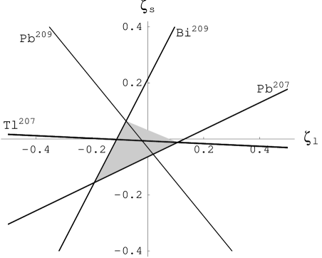
Figure 3: Region of allowed values for $\zeta_{l}$ and $\zeta_{s}$ with core polarization effects.

The resulting distribution of the magnetic moment density in ²⁰⁹Bi is shown in Fig. 4. The magnetization density is peaked near nuclear surface both for the bare contribution of the unpaired proton, shown by a dashed line, and for the total density shown by full line. The peak position in the total magnetization density is shifted slightly to smaller r. This is related directly to the decrease of $g_{s}$ inside the nucleus (see Fig. 1). The decrease leads to enhancement of the magnetic moment in this region due to opposite sign of the spin part of the magnetic moment relative to its orbital contribution for $h_{9/2}$ level. The shift of the peak results in some decrease of the magnetization rms-radius. The calculated magnetization rms-radius is practically insensitive to the values of $\zeta_{l}$ and $\zeta_{s}$ within the above range. It is equal to $\langle r_{m}^{2}\rangle^{1/2}=5.86$ fm. Fig. 5 gives similar figure for the octupole moment density distribution in ²⁰⁹Bi. In Figs. 4,5 one can see that the core polarization effects for the octupole moment are really larger than for the magnetic moment.

Figure 4: Magnetic moment density distribution in ²⁰⁹Bi. A contribution from a bare unpaired proton is shown by a dashed line. Full line shows the total magnetic moment density including core polarization.

Figure 5: Octupole moment density distribution in ²⁰⁹Bi. A contribution from a bare unpaired proton is shown by a dashed line. Full line shows the total octupole moment density including core polarization.

Table 3: Theoretical values of the ground-state hfs and the experimental results. The major contribution to uncertainties of the theoretical values originates from the uncertainties in the Bohr-Weisskopf effect.

$E_{hfs}$ in eV	209Bi82+	207Pb81+			$\epsilon$ for 209Bi82+	$\epsilon$ for 207Pb81+
$E_{0}$	5.191(5)	1.274(3)		Our work	0.0095$(\!\!\!{\scriptsize\begin{array}[]{c}+7\\ -38\end{array}}\!\!\!)$	0.0353$(\!\!\!{\scriptsize\begin{array}[]{c}-35\\ +164\end{array}}\!\!\!)$
$\Delta E_{BW}$	-0.050$(\!\!\!{\scriptsize\begin{array}[]{c}-3\\ +20\end{array}}\!\!\!)$	-0.045$(\!\!\!{\scriptsize\begin{array}[]{c}+4\\ -21\end{array}}\!\!\!)$		Shabaev et al. [11]	0.0118	0.0419
$\Delta E_{QED}$	-0.030	-0.007		Gustavsson et al. [12]	0.0131(26)	0.0429(86)
$E_{hfs}^{theory}$	5.111$(\!\!\!{\scriptsize\begin{array}[]{c}-3\\ +20\end{array}}\!\!\!)$(5)	1.222$(\!\!\!{\scriptsize\begin{array}[]{c}+4\\ -21\end{array}}\!\!\!)$(3)		Tomaselli et al. [15]	0.0210(17)	0.0289(15)
$E_{hfs}^{exper.}$	5.0840(8)	1.2159(2)		Experiment	0.0147(11)	0.0397(25)

The results obtained for hfs are listed in the left part of Table 3. Here $E_{0}$ corresponds to the relativistic Fermi formulae plus charge distribution correction. The uncertainty in the value of $E_{0}$ originates mainly from the uncertainty of the measured magnetic moment: $\mu=4.110(4)\mu_{N}$ for ²⁰⁹Bi and $\mu=0.5925(6)\mu_{N}$ for ²⁰⁷Pb [29]. The uncertainty of the charge distribution correction is small and can be neglected. The uncertainties in Bohr-Weisskopf effect $\Delta E_{BW}$ come from the uncertainties in the effective charges $\zeta_{s}$ and $\zeta_{l}$. They were determined using the shadow triangle shown in Fig. 3. They are not symmetric since the “best” values of $\zeta_{l}$ and $\zeta_{s}$ are lying close to ²⁰⁹Bi line in Fig. 3. In order to compare our calculations with the data we need $\Delta E_{QED}$. It was calculated in several papers and the results are consistent [11, 16, 17, 18, 19]. In [19] it was shown that $\Delta E_{QED}$ is insensitive to details of the magnetization distribution. They give for $\Delta E_{QED}$ the value $\Delta E_{QED}=-0.0298(3)$ eV for ²⁰⁹Bi⁸²⁺ and $\Delta E_{QED}=-0.00726(7)$ eV for ²⁰⁷Pb⁸¹⁺. In our calculated values of the ground-state hfs $E_{hfs}^{theory}$ the uncertainty in the first brackets originates from $\Delta E_{BW}$ and the second one originates from $\Delta E_{QED}$. The right part of the Table 3 gives our results for Bohr-Weisskopf effect in comparison with some other theoretical calculations. While our result for the ground-state hfs of ²⁰⁷Pb⁸¹⁺ is in good agreement with the data, the result for ²⁰⁹Bi⁸²⁺ lies out of the data. The calculated $\epsilon$ at its upper limit $\epsilon=0.0103$ differs by four standard deviations from the measured value $\epsilon=0.0147\pm 0.0011$. Actually, $\epsilon$ is not directly measured value. It was obtained from the measured $E^{exper.}_{hfs}$ using the calculated values of $E_{0}$ and $\Delta E_{QED}$. The uncertainty in $\epsilon$ comes mainly from the uncertainties in these calculated $E_{0}$. In other calculations only in [15] the particle-phonon coupling was accounted in scope of the DCM. In [11], and [12], and others (see Refs. in [12]) the unpaired particle was treated as an independent particle moving in a mean field potential. In this approach, the difference in $\epsilon$ reflects more the sensitivity to the choice of a particular mean field potential. It is interesting to note that $\epsilon$ calculated in [15] lies almost on the same distance from the experimental value, but on the other side compared to our value. This difference may be attributed to ground state correlations that contribute significantly to transition probabilities at small excitation energies [34]. In order to check whether our results is sensitive to a particular parameterization of the effective charges we made calculation of the hfs in ²⁰⁹Bi⁸²⁺ treating all the giromagnetic ratios $g_{l}(p),g_{l}(n),g_{s}(p),$ and $g_{s}(n)$ as free parameters. Their values were obtained by fitting the magnetic moments of four nuclei mentioned above. The magnetic moments were calculated together with the core polarization effects and the $ls$-corrections. With these new parameters we calculated hfs for ²⁰⁹Bi⁸²⁺ and obtained exactly the same result $\Delta E_{BW}=-0.050$ eV. This situation seems to be rather general. We changed different parameters entering in our theory, including $g$ and $g^{\prime}$, although $g^{\prime}$ is fixed by the position of Gamow-Teller resonances [35]. But, as soon as the magnetic moment of ²⁰⁹Bi is fitted, the correction $\Delta E_{BW}$ becomes close to the value cited in Table 3.

In addition to the magnetic moment, for ²⁰⁹Bi there are other observables related to the magnetic properties. In Table 4 we summarized our results including there our calculations of the octupole moment of ²⁰⁹Bi and the hfs in muonic ²⁰⁹Bi. To demonstrate the relative importance of the core polarization effects for different observables we made additional calculation switching off the core polarization and keeping the same parameterization of the effective charges via $\zeta_{l}$ and $\zeta_{s}$. One can see that although the effects of the core polarization are not very significant for the electronic hfs, for other observables, like the octupole moment, they are rather large. All the observables except the electronic hfs in ²⁰⁹Bi are in good agreement with the data. However, the experimental uncertainties in case of the octupole moment and the muonic hfs are rather large. It would be very desirable to reduce them in order to see whether the discrepancy in the electronic hfs in ²⁰⁹Bi were pronounced in these observables as well at higher accuracy of the data.

In summary, using continuum RPA with effective residual forces we calculated the distribution of the magnetic and the octupole densities for ²⁰⁹Bi. Additional contribution from velocity dependent spin-orbit two-particle interaction was calculated explicitly. The parameters of the theory were fixed by fitting the magnetic moments of four one-particle and one-hole nuclei around ²⁰⁸Pb. Basing on these results we calculated the hfs in hydrogen-like ²⁰⁹Bi⁸²⁺ and ²⁰⁷Pb⁸¹⁺ ions, the octupole magnetic moment in ²⁰⁹Bi, and hfs in muonic atom of ²⁰⁹Bi. Except the electronic hfs in hydrogen-like ²⁰⁹Bi⁸²⁺ all other results are in good agreement with experiment.

5 Acknowledgments

The authors appreciate the discussions with I.B. Khriplovich.

Table 4: Relative importance of the core polarization effects for different observables.

	Without core p. effects	With core p. effects	Experiment
$\Delta E_{BW}$ for 209Bi, eV	-0.046$(\!\!\!{\scriptsize\begin{array}[]{c}-3\\ +39\end{array}}\!\!\!)$	-0.050$(\!\!\!{\scriptsize\begin{array}[]{c}-3\\ +20\end{array}}\!\!\!)$
$E_{hfs}$ for 209Bi, eV	5.115$(\!\!\!{\scriptsize\begin{array}[]{c}-3\\ +39\end{array}}\!\!\!)$(5)	5.111$(\!\!\!{\scriptsize\begin{array}[]{c}-3\\ +20\end{array}}\!\!\!)$(5)	5.0840(8)
$\Delta E_{BW}$ for 207Pb, eV	-0.035$(\!\!\!{\scriptsize\begin{array}[]{c}+3\\ -37\end{array}}\!\!\!)$	-0.045$(\!\!\!{\scriptsize\begin{array}[]{c}+4\\ -21\end{array}}\!\!\!)$
$E_{hfs}$ for 207Pb, eV	1.232$(\!\!\!{\scriptsize\begin{array}[]{c}+3\\ -37\end{array}}\!\!\!)$(3)	1.222$(\!\!\!{\scriptsize\begin{array}[]{c}+4\\ -21\end{array}}\!\!\!)$(3)	1.2159(2)
$\Delta E_{BW}$ for muonic 209Bi, KeV	-1.73$(\!\!\!{\scriptsize\begin{array}[]{c}-9\\ +129\end{array}}\!\!\!)$	-1.86$(\!\!\!{\scriptsize\begin{array}[]{c}-10\\ +64\end{array}}\!\!\!)$
$E_{hfs}$ for muonic 209Bi, KeV	4.76$(\!\!\!{\scriptsize\begin{array}[]{c}-9\\ +129\end{array}}\!\!\!)$(6)	4.63$(\!\!\!{\scriptsize\begin{array}[]{c}-10\\ +64\end{array}}\!\!\!)$(6)	4.44(15)
Octupole moment of 209Bi, $\mu_{N}\cdot$fm2	-42$(\!\!\!{\scriptsize\begin{array}[]{c}-2\\ +30\end{array}}\!\!\!)$	-55$(\!\!\!{\scriptsize\begin{array}[]{c}-2\\ +16\end{array}}\!\!\!)$	-55(3)

Appendix A Spin-orbit corrections to the bare vertices

The vertex $\mathcal{M}_{JM}$ is the solution of equation (2) with the bare vertex (30). The Eqs. (3), (30) obtained using the standard electromagnetic current density for free nucleons. However, due to velocity dependence of the spin-orbit interaction (11), there are the corrections to electromagnetic current density. The corrections were discussed earlier [27, 20]. They produce an additional contributions to the bare vertexes $\mathcal{M}^{0}_{JM}$ and $\Gamma^{0}_{1\mu}$,

$$\Delta\mathcal{M}^{0p}_{JM}=\sqrt{4\pi J}\mu_{N}\frac{2mr^{2}_{0}}{\hbar^{2}}C\sum_{a}\left[-(\kappa+\kappa^{\prime})r^{J-1}_{a}\rho_{p}(r_{a})+(\kappa-\kappa^{\prime})\frac{1}{2J+1}r^{J}_{a}\frac{d\rho_{n}(r_{a})}{dr}\right]T^{(1)}_{JM}(a)$$

$$+(\kappa-\kappa^{\prime})\frac{1}{(2J+1)}\sqrt{\frac{J}{J+1}}r^{J}_{a}\frac{d\rho_{n}(r_{a})}{dr}T^{(2)}_{JM}(a),$$ (33)

$$\Delta\mathcal{M}^{0n}_{JM}=\sqrt{4\pi J}\mu_{N}\frac{2mr^{2}_{0}}{\hbar^{2}}C\sum_{a}\left[-(\kappa-\kappa^{\prime})r^{J-1}_{a}\rho_{p}(r_{a})-(\kappa-\kappa^{\prime})\frac{1}{2J+1}r^{J}_{a}\frac{d\rho_{p}(r_{a})}{dr}\right]T^{(1)}_{JM}(a)$$

$$-(\kappa-\kappa^{\prime})\frac{1}{(2J+1)}\sqrt{\frac{J}{J+1}}r^{J}_{a}\frac{d\rho_{p}(r_{a})}{dr}T^{(2)}_{JM}(a).$$ (34)

$$\Delta\Gamma^{0p}_{1\mu}=\frac{4eK}{j+1}\frac{2I+1}{2I}\left\{\Delta\mathcal{M}^{0p}_{1\mu}\,\Omega^{(0)}_{nlj}-\sqrt{4\pi}\mu_{N}\frac{2mr^{2}_{0}}{\hbar^{2}}C\sum_{a}\left[-\left((\kappa+\kappa^{\prime})\rho_{p}(r_{a})-\frac{1}{3}(\kappa-\kappa^{\prime})r_{a}\frac{d\rho_{n}(r_{a})}{dr}\right)\Omega^{(1)}_{nlj}(r_{a})\right.\right.$$

$$\left.-\frac{1}{3}(\kappa-\kappa^{\prime})r_{a}\frac{d\rho_{n}(r_{a})}{dr}\Omega^{(2)}_{nlj}(r_{a})\right]T^{(1)}_{1\mu}(a)+\left[\frac{1}{3}(\kappa-\kappa^{\prime})r_{a}\frac{d\rho_{n}(r_{a})}{dr}\Omega^{(1)}_{nlj}(r_{a})\right.$$

$$\left.\left.-\left((\kappa+\kappa^{\prime})\rho_{p}(r_{a})+\frac{1}{3}(\kappa-\kappa^{\prime})r_{a}\frac{d\rho_{n}(r_{a})}{dr}\right)\Omega^{(2)}_{nlj}(r_{a})\right]\sqrt{\frac{1}{2}}T^{(2)}_{1\mu}(a)\right\},$$ (35)

$$\Delta\Gamma^{0n}_{1\mu}=\frac{4eK}{j+1}\frac{2I+1}{2I}\left\{\Delta\mathcal{M}^{0n}_{1\mu}\,\Omega^{(0)}_{nlj}-\sqrt{4\pi}\mu_{N}\frac{2mr^{2}_{0}}{\hbar^{2}}C\sum_{a}\left[-\left((\kappa-\kappa^{\prime})\rho_{p}(r_{a})+\frac{1}{3}(\kappa-\kappa^{\prime})r_{a}\frac{d\rho_{p}(r_{a})}{dr}\right)\Omega^{(1)}_{nlj}(r_{a})\right.\right.$$

$$\left.+\frac{1}{3}(\kappa-\kappa^{\prime})r_{a}\frac{d\rho_{p}(r_{a})}{dr}\Omega^{(2)}_{nlj}(r_{a})\right]T^{(1)}_{1\mu}(a)+\left[-\frac{1}{3}(\kappa-\kappa^{\prime})r_{a}\frac{d\rho_{p}(r_{a})}{dr}\Omega^{(1)}_{nlj}(r_{a})\right.$$

$$\left.\left.+\left(-(\kappa-\kappa^{\prime})\rho_{p}(r_{a})+\frac{1}{3}(\kappa-\kappa^{\prime})r_{a}\frac{d\rho_{p}(r_{a})}{dr}\right)\Omega^{(2)}_{nlj}(r_{a})\right]\sqrt{\frac{1}{2}}T^{(2)}_{1\mu}(a)\right\}.$$ (36)

References

- [1] I. Klaft, S. Borneis, T. Engel, B. Fricke, R. Grieser, G. Huber, T. Kühl, D. Marx, R. Neumann, S. Schröder, P. Seelig, and L. Völker, Phys. Rev. Lett. 73 (1994) 2425.
- [2] E. Fermi, Zeitschrift für Physsik 60 (1930) 320.
- [3] G. Breit, Phys. Rev. 35 (1930) 1447.
- [4] J. E. Rosenthal and G. Breit, Phys. Rev. 41 (1932) 459.
- [5] M. F. Crawford and A. K. Schawlow, Phys. Rev. 76 (1949) 1310.
- [6] H. J. Rosenberg and H. H. Stroke, Phys. Rev. A 5 (1972) 1992.
- [7] H. de Vries, C. W. de Jager, and C. de Vriex, At. Data Nuclear Data Tables 36 (1987) 495.
- [8] V. M. Shabaev, J. Phys. B 27 (1994) 5825.
- [9] A. Bohr and V. F. Weisskopf, Phys. Rev. 77 (1950) 94.
- [10] A. Bohr, Phys. Rev. 81 (1951) 331.
- [11] V. M. Shabaev, M. Tomaselli, T. Kühl, A. N. Artemyev, and V.A. Yerokhin, Phys. Rev. A 56 (1997) 252.
- [12] M. G. N. Gustavsson, C. Forssén, and A.-M. Mårtensson-Pendrill, Hyperfine Interactions 127 (2000) 347.
- [13] L. N. Labzowsky, W. R. Johnson, S. M. Schneider, and G. Soff, Phys. Rev. A 51 (1995) 4597.
- [14] M. Tomaselli, S. M. Schneider, E. Kankeleit, and T. Kühl, Phys. Rev. C 51 (1995) 2989.
- [15] M. Tomaselli, T. Kühl, P. Seelig, C. Holbrow, and E. Kankeleit, Phys. Rev. C 58 (1998) 1524.
- [16] S. M. Schneider, W. Greiner, and G. Soff, Phys. Rev. A 50 (1994) 118.
- [17] H. Persson, S. M. Schneider, W. Greiner, G. Soff, and I. Lindgren, Phys. Rev. Lett. 76 (1996) 1433.
- [18] S. A. Blundell, K. T. Cheng, and J. Sapirstein, Phys. Rev. A 55 (1997) 1857.
- [19] P. Sunnergren, H. Persson, S. Salomonson, S. M. Schneider, G. Soff, and I. Lindgren, Phys. Rev. A 58 (1998) 1055.
- [20] V. F. Dmitriev and V. B. Telitsin, Nucl. Phys. A 402 (1983) 581.
- [21] A. B. Migdal, Theory of finite Fermi system (Wiley Interscience, New York, 1967).
- [22] J. Speth, E. Werner, and W. Wild, Phys. Reports C 33(3) (1977) 127.
- [23] S. Shlomo and G. Bertsch, Nucl. Phys. A 243 (1975) 507.
- [24] E. E. Sapershtein, C. A. Fajans, and V. A. Chodel, Fis. Elem. Chast. i Atom. Yad. [Sov. J. Particles and Nuclei] 9 (1978) 221.
- [25] A. Arima and H. Hori, Prog. Theor. Phys. 12 (1954) 623.
- [26] D. A. Varshalovich et al., Kvantovaya teoriya uglovogo momenta (Nauka, Leningrad, 1975).
- [27] A. Bohr, B.R. Mottelson, Nuclear Structure, v.1 (W.A. Benjamin, Inc., NY, Amsterdam, 1969).
- [28] B.L. Birbrair, V.A. Sadovnikova, Yadernaja Fizika 188 (1974) 1815.
- [29] M. G. N. Gustavsson and A.-M. Mårtensson-Pendrill, Phys. Rev. A 58 (1998) 3611.
- [30] D.A. Landman, A. Lurio, Phys. Rev. A 1 (1970) 1330.
- [31] N.J. Stone,Table of Nuclear Moments (http://www.nndc.bnl.gov/nndc/stone_moments, 2001).
- [32] P. Seelig et al., Phys. Rev. Lett. 81 (1998) 4824.
- [33] A. Rüetschi et al., Nucl. Phys. A 422 (1986) 461.
- [34] G.E. Brown, Unified Theory of Nuclear Models and Forces (North-Holland, Amsterdam, 1967).
- [35] F. Osterfeld, Rev. Mod. Phys., 64 (1992) 491.