Kaon and Pion Fluctuations from Small Disoriented Chiral Condensates

Abstract

Enhancement of $\Omega$ and $\overline{\Omega}$ baryon production in Pb+Pb collisions at a c.m. energy of 17 $A$ GeV can be explained by the formation of many small disoriented chiral condensate regions. This explanation implies that neutral and charged kaons as well as pions must exhibit novel isospin fluctuations. We compute the distribution of the fraction of neutral pions and kaons from such regions. We then propose robust statistical observables that can be used to extract the novel fluctuations from background contributions in $\pi^{0}\pi^{\pm}$ and $K_{S}^{0}K^{\pm}$ measurements at RHIC and LHC.

]

I Introduction

Heavy ion collisions at the Brookhaven Relativistic Heavy Ion Collider (RHIC) at center of mass energies up to $200$ $A$ GeV and the CERN Large Hadron Collider (LHC) at $5.5$ $A$ TeV may produce matter in which chiral symmetry is restored. One possible consequence of the restoration and the subsequent re-breaking of chiral symmetry is the formation of disoriented chiral condensates (DCC) – transient regions in which the average chiral order parameter differs from its value in the surrounding vacuum [1, 2, 3].

Measurements of $\Omega$ and $\overline{\Omega}$ baryon enhancement [4] at $17$ $A$ GeV at the CERN SPS can be explained by the production of many small DCC regions within individual collision events [5]. If true, this explanation has two important consequences. First, the DCC regions must be rather small, with a size of about $2$ fm. Such a size is consistent with predictions based on dynamical simulations of the two flavor linear sigma model [6]. More startling is the second implication that the evolution of the condensate can have a significant effect on strange particle production. The importance of strange degrees of freedom in describing chiral restoration has been long appreciated [7, 8, 9, 10, 11], but simulations of the three flavor linear sigma model had suggested that strange kaon fields are much less important than the pion fields [12]. Nevertheless, the $\Omega$ and $\overline{\Omega}$ data demand that we explore without prejudice techniques for measuring kaon fluctuations.

In this paper we study pion and kaon isospin fluctuations in the presence of many small DCC. In the next section we compute probability distributions that describe the DCC contribution to these fluctuations. Pion fluctuations due to many small DCC have been addressed by Amado and Lu [13] and Chow and Cohen [14], although the distribution we compute is new. Ours is the first work to study kaon fluctuations. In sec. 3 we combine the DCC fluctuations with a contribution from a random thermal background. In sec. 4 we discuss how the size and number of DCC vary with impact parameter, target and projectile size. In sec. 5 we assess robust statistical observables that can be used to measure the impact of many small DCC at RHIC and LHC. In particular, we obtain a dynamic isospin fluctuation observable analogous to the dynamic charge observable used to measure net charge fluctuations at RHIC [15]. Of the quantities considered, this observable isolates the DCC effect from other sources of fluctuations best.

To illustrate how a strange DCC can form, we first consider QCD with only up and down quark flavors. Equilibrium high temperature QCD respects chiral symmetry if the quarks are taken to be massless. This symmetry is broken below $T_{c}\sim 150$ MeV by the formation of a chiral condensate $\langle\sigma\rangle\sim\langle\overline{u}u+\overline{d}d\rangle$ that is a scalar isopin singlet. However, chiral symmetry implies that $\sigma$ is degenerate with a pseudoscalar isospin triplet of fields with the same quantum numbers as the pions. In reality, chiral symmetry is only approximate and the 140 MeV pion mass is different from the $800\pm 400$ MeV mass of the leading sigma candidate [16]. Nevertheless, lattice calculations exhibit a dramatic drop of $\langle\sigma\rangle$ near $T_{c}$ at finite quark masses.

A DCC can form when a heavy ion collision produces a high energy density quark-gluon system that then rapidly expands and cools through the critical temperature. Such a system can initially break chiral symmetry along one of the pion directions, but must then evolve to the $T=0$ vacuum by radiating pions. A single coherent DCC radiates a fraction $f_{\pi}$ of neutral pions compared to the total that satisfies the probability distribution

$$\rho_{1}(f_{\pi})={{1}\over{2f_{\pi}^{1/2}}}\,\,\,\,\,\,\,\,\,\,\,\,\,\,\,\,0<f_{\pi}\leq 1,$$ (1)

[17, 18, 19]. Such isospin fluctuations constitute the primary signal for DCC formation. The enhancement of baryon-antibaryon pair production is a secondary effect due to the relation between baryon number and the topology of the pion condensate field [20].

This two flavor idealization only applies if the strange quark mass $m_{s}$ can be taken to be infinite. Alternatively, if we take $m_{s}=m_{u}=m_{d}=0$, then the chiral condensate would be an up-down-strange symmetric scalar field. The more realistic case of $m_{s}\sim 100$ MeV is between these extremes, so that $\langle\sigma\rangle\sim\langle\cos\theta(\overline{u}u+\overline{d}d)+\sin\theta(\overline{s}s)\rangle$. The mixing angle $\theta$ is highly uncertain since it depends on the sigma mass together with the $\pi,K,\eta$ and $\eta^{\prime}$ masses and the $\eta-\eta^{\prime}$ mixing angle [9]. A disoriented condensate can evolve by radiating $\pi,K,\eta$ and $\eta^{\prime}$ mesons, with the neutral pion fraction satisfying (1). Randrup and Schäffner-Bielich find that the kaon fluctuations from a single large DCC satisfy [12]

$$\rho_{1}(f_{K})=1\,\,\,\,\,\,\,\,\,\,\,\,\,\,\,\,0\leq f_{K}\leq 1,$$ (2)

where $f_{K}=(K^{0}+\overline{K}^{0})/(K^{+}+K^{-}+K^{0}+\overline{K}^{0})$. Moreover, the condensate fluctuations can now produce strange baryon pairs [5]. Linear sigma model simulations indicate that pion fluctuations dominate three-flavor DCC behavior, while the fraction of energy imparted to kaon fluctuations is very small due to the kaons’ larger mass. On the other hand, domain formation may be induced by other mechanisms such as bubble formation [21] or decay of the Polyakov loop condensate [22].

Why does the DCC’s size matter? Pion measurements in individual collision events can distinguish DCC isospin fluctuations from a thermal background only if the disoriented region is sufficiently large [2]. DCC can then be the dominant source of pions at low transverse momenta, since $\langle p_{t}\rangle\sim 1/R$ for a coherent region of size $R$. Experiments focusing on low $p_{t}$ can study neutral and charged pion fluctuations [19], wavelet [23] and HBT signals [2, 24] to extract detailed information. In contrast, for small domains ($R<3$ fm [2]) DCC signals are hidden by fluctuations due to ordinary incoherent production mechanisms. This holds even if many such regions are produced per event. DCC mesons from small regions may have momenta of a few hundred MeV, nearer the $pp$ mean value. Different regions would not add coherently to alter HBT, nor would their small spatial structures affect wavelet analyses.

Importantly, baryon pair enhancement is substantial only if there are many small incoherent regions. The large winding numbers that produce baryon-antibaryon pairs require many small regions with random relative orientations of the pion field. To describe strange antibaryon enhancement, Kapusta and Wong assume roughly 100 DCC regions of size of roughly $2$ fm [5]. Topological models of baryon-antibaryon pair production successfully describe $e+e-$ and hadronic collision data [25]. The connection of DCC to topological pair production was pointed out in Ref. [20]; see also [26].

II Fluctuations in Neutral DCC Mesons

In this section we will compute the statistical distribution of the ratio of neutral to total number of mesons, first for kaons and then for pions. In both cases the limit that the number of DCC domains becomes large is taken. It is natural that this limit results in a Gaussian distribution for both kaons and pions on account of the Central Limit Theorem. In the next section these distributions will be folded together with a random or thermal source which most likely would comprise the bulk of the mesons in a high energy heavy ion collision.

A Kaons

Define $f=(K^{0}+\overline{K}^{0})/(K^{+}+K^{-}+K^{0}+\overline{K}^{0})$. To an excellent approximation the number of neutral kaons is equal to twice the number of short-lived neutral kaons $K_{S}$ which are more readily measurable in high energy heavy ion collisions. The fraction $f$ ranges from 0 to 1.

The statistical distribution in $f$ for a single domain is $\rho_{1}(f)=1$. The distribution for $n$ randomly oriented, independent domains is

$$\rho_{n}(f)=\int\prod_{k=1}^{n}df_{k}\,\rho_{1}(f_{k})\,\delta\left(f-\frac{1}{n}\sum_{j=1}^{n}f_{j}\right)\,.$$ (3)

The Dirac delta function can be represented as an integral. Then $\rho_{n}$ can be written as

$$\rho_{n}(f)=\int_{-\infty}^{\infty}\frac{dz}{2\pi}e^{-ifz}\left[\int_{0}^{1}dx\rho_{1}(x)e^{ixz/n}\right]^{n}\,.$$ (4)

Since $\rho_{1}(f)=1$, the integration over $x$ can be done, resulting in a one- dimensional integral.

$$\rho_{n}(f)=\frac{n}{\pi}\int_{-\infty}^{\infty}dt\left(\frac{\sin t}{t}\right)^{n}\cos\left[n(1-2f)t\right]$$ (5)

The integral can be evaluated and expressed in terms of a finite sum.

$$\rho_{n}(f)=n^{2}\sum_{0\leq k<n(1-f)}(-1)^{k}\frac{[n(1-f)-k]^{n-1}}{k!(n-k)!}$$ (6)

It is useful to have a simple analytic formula for $\rho_{n}$ in the limit that $n\gg 1$. In this limit the factor $(\sin t/t)^{n}$ in the integral formula is strongly peaked at $t=0$. Let us write this factor as $\exp(-F(t))$ with a view towards a saddle point approximation. We get

$$F(0) = F^{\prime}(0)=0$$ (7)

$$F^{\prime\prime}(0) = n/3$$ (8)

$$e^{-F(t)} \approx e^{-nt^{2}/6}\,.$$ (9)

Use of this approximation yields the asymptotic formula

$$\rho_{n}(f)=\sqrt{\frac{6n}{\pi}}\exp[-6n(f-1/2)^{2}]\,.$$ (10)

The distribution is strongly peaked around $f=1/2$ as one might expect.

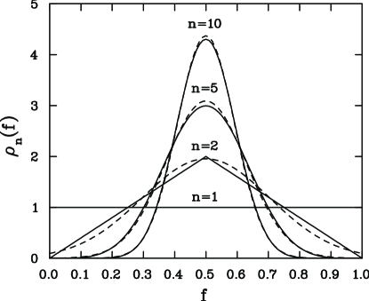
FIG. 1.: The probability distribution for the ratio of neutral to total number of DCC kaons from $n$ domains. The dashed curves represent Gaussian distributions. From eqs. (6) and (8).

Figure 1 shows the evolution of $\rho_{n}(f)$ with $n$. It goes from a flat distribution for $n=1$ to a Gaussian sharply peaked at $f=1/2$ as $n$ becomes large compared to 1. In fact a Gaussian is a very good representation for $n>2$.

B Pions

Define $f=\pi^{0}/(\pi^{+}+\pi^{-}+\pi^{0})$. To a good approximation the number of neutral pions is equal to half the number of photons. Therefore, to this level of precision, it is not necessary to identify each $\pi^{0}$ via its decay into $2\gamma$. The fraction $f$ ranges from 0 to 1.

The statistical distribution in $f$ for a single domain is $\rho_{1}(f)=1/2\sqrt{f}$. The distribution for $n$ randomly oriented, independent domains can be computed along the same lines as for kaons.

$$\rho_{n}(f)=\int_{-\infty}^{\infty}\frac{dz}{2\pi}e^{-ifz}\left[\int_{0}^{1}\frac{dx}{2\sqrt{x}}e^{ixz/n}\right]^{n}\,.$$ (11)

Since pions from DCC have been extensively studied we shall be content to evaluate the distribution in the large $n$ limit. This is accomplished by expanding the exponential in the $x$ integration to second order in $1/n$, evaluating the resulting integrals, and exponentiating. Thus

$$\int_{0}^{1}\frac{dx}{2\sqrt{x}}e^{ixz/n}\approx\exp\left[i\frac{z}{3n}-\frac{2z^{2}}{45n^{2}}\right]\,.$$ (12)

The $z$ integral can then be done, yielding a Gaussian centered at $f=1/3$.

$$\rho_{n}(f)=\sqrt{\frac{45n}{4\pi}}\exp\left[-45n(f-1/3)^{2}/4\right]$$ (13)

III Folding DCC and Thermal Mesons

In a more realistic scenario some kaons will come from the decay or realignment of DCC domains and some will come from more conventional sources. We shall refer to the latter as random or thermal, even though that may be a bit of a misnomer. What we mean by random or thermal is that the distribution of kaons from non-DCC sources is

$$\rho_{0}(f_{0})=\frac{1}{2\pi\sigma_{0}^{2}}\exp\left[-(f_{0}-1/2)^{2}/2\sigma_{0}^{2}\right]\,.$$ (14)

For a completely random source the width $\sigma_{0}$ is related to the total number $N_{\rm random}$ of non-DCC kaons by

$$\sigma^{2}_{0}=\frac{1/2(1-1/2)}{N_{\rm random}}=\frac{1}{4N_{\rm random}}\,.$$ (15)

Now let us assume that a fraction $\alpha_{K}$ of all kaons come from non-DCC sources and the remaining fraction $\beta_{K}=1-\alpha_{K}$ come from $n\gg 1$ independent DCC domains. Letting $N$ denote the total number of kaons, we have $N_{\rm random}=\alpha_{K}N$ and $N_{\rm DCC}=\beta_{K}N$. Folding together two Gaussians gives a Gaussian.

$$\rho_{K}(f) = \int df_{0}df_{n}\rho_{0}(f_{0})\rho_{n}(f_{n})\delta(f-\alpha_{K}f_{0}-\beta_{K}f_{n})$$ (16)

$$= \frac{1}{\sqrt{2\pi\Delta_{K}^{2}}}\exp\left[-(f-1/2)^{2}/2\Delta_{K}^{2}\right]$$ (17)

The net width is

$$\Delta_{K}^{2}=\frac{\alpha_{K}}{4N}+\frac{\beta_{K}^{2}}{12n}=\frac{1}{4N}+\left\{\frac{\beta_{K}^{2}}{12n}-\frac{\beta_{K}}{4N}\right\}\,.$$ (18)

The expression in curly brackets at the end represents the difference between the actual width and the width the distribution would have if there was no contribution from DCC kaons. This change in the width may be positive or negative, depending on the parameters.

An analogous analysis can be given for pions. This results in the distribution

$$\rho_{\pi}(f) = \int df_{0}df_{n}\rho_{0}(f_{0})\rho_{n}(f_{n})\delta(f-\alpha_{\pi}f_{0}-\beta_{\pi}f_{n})$$ (19)

$$= \frac{1}{\sqrt{2\pi\Delta_{\pi}^{2}}}\exp\left[-(f-1/3)^{2}/2\Delta_{\pi}^{2}\right]$$ (20)

with a net width of

$$\Delta_{\pi}^{2}=\frac{2\alpha_{\pi}}{9N}+\frac{2\beta_{\pi}^{2}}{45n}=\frac{2}{9N}+\left\{\frac{2\beta_{\pi}^{2}}{45n}-\frac{2\beta_{\pi}}{9N}\right\}\,.$$ (21)

As with the kaons, the last expression in curly brackets represents the difference between the actual width and the width the distribution would have if there was no contribution from DCC pions. Note that the fractions $\alpha_{K}$ and $\alpha_{\pi}$ need not be the same.

IV Volume or Surface Scaling?

The issue we wish to address is whether the number of DCC mesons (kaons or pions) scales with the volume or surface area of the system. This is an important issue when studying the impact parameter dependence or the dependence on the size of the projectile and target nuclei.

In this paper it is assumed that DCC have a typical size of order 2 fm which does not change much with collision energy or the total volume of the system. Thus the number of domains $n$ is just given by the ratio of the two volumes: $n=V_{\rm system}/V_{DCC}$. Scaling of the number of DCC kaons or pions, $N_{DCC}$, with $n$ or $V_{\rm system}$ is the same because the size of individual domains is fixed. The $N_{DCC}$ will depend on the extra energy associated with the formation of a domain. If the up and down quark masses were zero then QCD would have perfect SU(2) flavor symmetry. In that case the energy density of a large uniform domain would be independent of its orientation. All directions in chiral space are equivalent. However, the misalignment between adjacent domains results in a surface energy, and so the number of DCC pions would be proportional to the total surface energy between domains. The up and down quark masses are not zero (they’re about 5 to 7 MeV), and this will result in an excess volume energy too. For pions one might expect the surface energy to dominate since the up and down quark masses are so small. For kaons one might expect the volume and surface energy contributions to be comparable on account of relatively large mass of the strange quark (about 120 MeV).

Let us analyze the scaling of the excess surface energy more quantitatively. Consider a cube with sides of length $L$ into which fit $n=(L/l)^{3}$ cubic domains, each with sides of length $l$. Assuming that each domain is oriented independently of its neighbors, the total surface energy scales with the total surface area, which is $3\left(\frac{L}{l}+1\right)\frac{L^{2}}{l^{2}}$. With $L\gg l$, and with the domain size $l$ fixed, the total surface area, energy, and therefore number of DCC mesons scale with $n$ to the power of one. Thus $N_{DCC}\propto n\propto V_{\rm system}$ no matter whether one imagines the excess energy being associated with domain interfaces or with domain interiors.

V Statistical Analysis

Detection of small incoherent DCC regions in high energy heavy ion collisions requires a statistical analysis in the $\pi^{0}\pi^{\pm}$ or the $K_{S}^{0}K^{\pm}$ channels. Neutral mesons can be detected by the decays $\pi^{0}\rightarrow\gamma\gamma$ or $K^{0}_{S}\rightarrow\pi^{+}\pi^{-}$. The analysis we propose is sensitive to correlations due to isospin fluctuations. We expect these correlations to vary when DCC regions increase in abundance or size as centrality, ion-mass number $A$, or beam energy are changed. Correlation results combined with other signals, such as baryon enhancement [5], can be used to build a circumstantial case for DCC production.

Correlations of $\pi^{0}\pi^{\pm}$ and $K_{S}^{0}K^{\pm}$ can be determined by measuring the robust isospin covariance,

$$R_{c0}={{\langle N_{c}N_{0}\rangle-\langle N_{c}\rangle\langle N_{0}\rangle}\over{\langle N_{c}\rangle\langle N_{0}\rangle}},$$ (22)

where $N_{0}$ and $N_{c}$ are the number of neutral and charged mesons. We take $N_{0}=N_{\pi^{0}}$ and $N_{c}=N_{\pi^{+}}+N_{\pi^{-}}$ for pion fluctuations and $N_{0}=2N_{K^{0}_{S}}$ and $N_{c}=N_{K^{+}}+N_{K^{-}}$ for kaon fluctuations. The ratio (18) has two features that are convenient for experimental determination. First, this observable is independent of detection efficiency as are the “robust” ratios discussed in [27]. Robust observables are useful for DCC studies because charged and neutral particles are identified using very different techniques and, consequently, are detected with different efficiency. Observe that robust quantities are not affected by the unobserved $K_{L}^{0}$, since the strong-interaction eigenstates $K^{0}$ and ${\overline{K}}^{0}$ are a superposition $K_{L}^{0}$ and $K_{S}^{0}$ until their decay well outside the collision region. Second, since (18) is obtained from a statistical analysis, individual $\pi^{0}\rightarrow\gamma\gamma$ or $K^{0}_{S}\rightarrow\pi^{+}\pi^{-}$ need not be fully reconstructed in each event. This feature is crucial because it would be extraordinarily difficult – if not impossible – to reconstruct a low momentum $\pi^{0}$ in heavy ion collisions except on a statistical basis.

Next we define robust variance

$$R_{aa}={{\langle N_{a}^{2}\rangle-\langle N_{a}\rangle^{2}-\langle N_{a}\rangle}\over{\langle N_{a}\rangle^{2}}},$$ (23)

where $a=c$ or 0. To see why (19) is robust, denote the probability of detecting each meson $\epsilon$ and the probability of missing it $1-\epsilon$. For a binomial distribution the average number of measured particles is $\langle N_{a}\rangle^{\rm exp}=\epsilon\langle N_{a}\rangle$ while the average square is $\langle N_{a}^{2}\rangle^{\rm exp}=\epsilon^{2}\langle N_{a}^{2}\rangle+\epsilon(1-\epsilon)\langle N_{a}\rangle$. We then find

$$R_{aa}^{\rm exp}=R_{aa},$$ (24)

independent of $\epsilon$ [28]; the proof that (18) is robust is similar. The ratios (18) and (19) are strictly robust only if the efficiency $\epsilon$ is independent of multiplicity. Further properties and advantages of these and similar quantities are discussed in [28].

To study DCC fluctuations we define the dynamic isospin observable

$$\nu_{\rm dyn}^{c0}=R_{cc}+R_{00}-2R_{c0}.$$ (25)

Analogous observables have been employed to study net charge fluctuations in particle physics [29, 30] and were considered in a heavy ion context in [15] and [31]. This quantity can be written in terms of

$$\nu^{c0}=\left\langle\left({{N_{0}}\over{\langle N_{0}\rangle}}-{{N_{c}}\over{\langle N_{c}\rangle}}\right)^{2}\right\rangle.$$ (26)

To isolate the dynamical isospin fluctuations from other sources of fluctuations, one obtains (21) by subtracting from (22) the uncorrelated Poisson limit $\nu_{\rm stat}^{c0}=\langle N_{0}\rangle^{-1}+\langle N_{c}\rangle^{-1}$. Indeed, we show in (27) below that the quantity (21) depends primarily on the fluctuations of the neutral fraction $f$, while the individual ratios (18) and (19) have additional contributions.

We illustrate the effect of DCC on the dynamic isospin fluctuations by writing $N_{0}=fN$ and $N_{c}=(1-f)N$. Small fluctuations on $f$ or $N$ results in the changes

$$\frac{\Delta N_{0}}{\langle N_{0}\rangle} = {{\Delta N}\over{\langle N\rangle}}+{{\Delta f}\over{\langle f\rangle}}\,,$$ (27)

$$\frac{\Delta N_{c}}{\langle N_{c}\rangle} = {{\Delta N}\over{\langle N\rangle}}-{{\Delta f}\over{1-\langle f\rangle}}\,.$$ (28)

We obtain the average

$${{\langle\Delta N_{0}^{2}\rangle}\over{\langle N_{0}\rangle^{2}}}=v+{{2c}\over{\langle N\rangle\langle f\rangle}}+{{\Delta^{2}}\over{\langle f\rangle^{2}}}\,.$$ (29)

Here the contribution of the variance of the total number of mesons is $v\equiv\langle\Delta N^{2}\rangle/\langle N\rangle^{2}$ and the charge-total covariance is $c\equiv\langle\Delta N\Delta f\rangle$. DCC formation primarily effects the charge fluctuation contribution, $\Delta^{2}\equiv\langle(\Delta f)^{2}\rangle$, from (15) or (17). Similarly,

$${{\langle\Delta N_{c}^{2}\rangle}\over{\langle N_{c}\rangle^{2}}}=v-{{2c}\over{\langle N\rangle(1-\langle f\rangle)}}+{{\Delta^{2}}\over{(1-\langle f\rangle)^{2}}}\,,$$ (30)

and

$$R_{c0}=v+\left({{1}\over{\langle f\rangle}}-{{1}\over{1-\langle f\rangle}}\right){{c}\over{\langle N\rangle}}-{{\Delta^{2}}\over{(1-\langle f\rangle)^{2}}}\,$$ (31)

where $R_{c0}$ is given by (18). Using (21) we get

$$\nu_{\rm dyn}^{c0}={{1}\over{\langle f\rangle(1-\langle f\rangle)}}\left({{\Delta^{2}}\over{\langle f\rangle(1-\langle f\rangle})}-{{1}\over{\langle N\rangle}}\right).$$ (32)

This observable isolates the isospin fluctuations, whereas the individual $R_{ab}$ depend on the fluctuations in total meson number, $v$ and $c$ as well.

We estimate the effect of DCC on the dynamical fluctuations (27) using (15) and (17). We take $\langle N\rangle=N_{K}$ for kaons and $\langle N\rangle=N_{\pi}$ for pions; these are the total number of mesons of the indicated kind. For kaons

$$\nu_{\rm dyn}^{c0}({\rm K~{}DCC})=4\beta_{K}\left(\frac{\beta_{K}}{3n}-\frac{1}{N_{K}}\right)\,,$$ (33)

and for pions

$$\nu_{\rm dyn}^{c0}(\pi~{}{\rm DCC})=4.5\beta_{\pi}\left(\frac{\beta_{\pi}}{5n}-\frac{1}{N_{\pi}}\right)\,.$$ (34)

These quantities can be positive or negative depending on the magnitude of $\beta$ compared to the number of domains per kaon. In fact the dynamical fluctuation may even be positive for one kind of meson and negative for the other.

How big is the DCC effect compared to alternative sources of fluctuations? In the absence of DCC $\alpha=1$ and $\beta=0$ so that (29) implies $\nu_{\rm dyn}^{c0}\equiv 0$ for both pions and kaons. On the other hand, in models which treat nuclear collisions as a superposition of independent nucleon-nucleon collisions, each nucleon-nucleon collision contributes an amount $\nu_{c0}^{pp}$ to the overall fluctuations. Consequently, $M$ nucleon-nucleon collisions can contribute an amount $\nu_{c0}^{pp}/M$ to the total $\nu_{\rm dyn}^{c0}$ [33]. While little is known from $pp$ experiments about kaon fluctuations, HIJING and RQMD models yield negative values of $\nu_{c0}^{pp}$. For kaons, HIJING simulations of central Au+Au at 200 $A$ GeV yield $\nu_{\rm dyn}^{c0}\approx-0.002$ for 47 $K^{+}$ and 44 $K_{S}^{0}$ on average [32]. The onset of a DCC contribution to $\nu_{\rm dyn}^{c0}$ can substantially change this value. A detailed of analysis of this problem within microscopic models will appear elsewhere [33].

VI Discussion and Conclusion

Reference [5] argued that the anomalous abundance and transverse momentum distributions of $\Omega$ and $\overline{\Omega}$ baryons in central collisions between Pb nuclei at 17 $A$ GeV at the CERN SPS is evidence that they are produced as topological defects arising from the formation of many domains of disoriented chiral condensates (DCC) with an average domain size of about 2 fm. Motivated by this interpretation, we have studied the effect of DCC on the distribution of the fractions of neutral kaons and pions. We showed that the distributions are accurately described by Gaussians with centroids at $f$ = 1/2 and 1/3, respectively, once the number of domains exceeds just a few. Folding together kaons or pions arising from DCC with other sources that are Gaussian distributed results once again in Gaussians. These may have a width that is greater or less than a purely random source without DCC formation.

The DCC pioneers [17, 18, 19, 1] had hoped that a large percentage of pions might be emitted from just a few big domains, on the order of 5 to 8 fm (kaons were not considered). Such large domains have been ruled out at SPS [3], but remain possible at RHIC. More conservatively, as the number of domains grow and their average size diminishes, the impression left on the fluctuations in the neutral fraction becomes more subtle and less unique. For many small domains, statistical measurements of both neutral kaons (pions) and charged kaons (pions) are needed. Since not every hadron emitted can possibly be detected with 100% efficiency, and since the experimental techniques that identify $K_{S}$, $K^{\pm}$, $\pi^{0}$ and $\pi^{\pm}$ are very different, we have identified robust observables that are essentially independent of all these uncertainties. In particular, we propose that the dynamical isospin observable (21) can be parameterized as in eqs. (28) and (29). DCC effects can appear as changes in the magnitude of the dynamical isospin observable as centrality is varied. We emphasize that similar consequence may follow from any mechanism that produces many small domains that decay to pions and kaons, such as the Polyakov Loop Condensate [22]. We anxiously await what RHIC will have to say!

REFERENCES

- [1] K. Rajagopal and F. Wilczek, Nucl. Phys. B399, 395 (1993); B404, 577 (1993); K. Rajagopal, in Quark-Gluon Plasma 2, R. C. Hwa ed., (World Scientific, 1995); hep-ph/9504310.
- [2] S. Gavin, Nucl. Phys. A590, 163c (1995).
- [3] T. Nayak, et al. (WA98 Collaboration), Nucl. Phys. A638, 249c (1998).
- [4] J. B. Kinson, J. Phys. G 25, 143 (1999).
- [5] J. I. Kapusta and S. M. Wong, Phys. Rev. Lett. 86, 4251 (2001); nucl-th/0012006.
- [6] S. Gavin, A. Gocksch and R. D. Pisarski, Phys. Rev. Lett. 72, 2143 (1994); hep-ph/9310228.
- [7] R. D. Pisarski and F. Wilczek, Phys. Rev. D 29, 338 (1984).
- [8] F. R. Brown et al., Phys. Rev. Lett. 65, 2491 (1990).
- [9] S. Gavin, A. Gocksch and R. D. Pisarski, Phys. Rev. D 49, 3079 (1994); hep-ph/9311350.
- [10] C. Schmidt, F. Karsch and E. Laermann, hep-lat/0110039.
- [11] J. T. Lenaghan, D. H. Rischke and J. Schaffner-Bielich, Phys. Rev. D 62, 085008 (2000); nucl-th/0004006.
- [12] J. Schaffner-Bielich and J. Randrup, Phys. Rev. C 59, 3329 (1999); nucl-th/9812032.
- [13] R. D. Amado and Y. Lu, Phys. Rev. D 54, 7075 (1996); hep-ph/9608242.
- [14] C. K. Chow and T. D. Cohen, Phys. Rev. C 60, 054902 (1999); nucl-th/9908013.
- [15] S. A. Voloshin [STAR Collaboration], nucl-ex/0109006.
- [16] D. E. Groom et al. [Particle Data Group Collaboration], Eur. Phys. J. C 15, 1 (2000).
- [17] A. A. Anselm and M. G. Ryskin, Phys. Lett. B266, 482 (1991).
- [18] J.-P. Blaizot and A. Kryzywicki, Phys. Rev. D 46, 246 (1992).
- [19] J. D. Bjorken, K. L. Kowalski and C. C. Taylor, Report SLAC-PUB-6109 (1993), hep-ph/9309235, unpublished.
- [20] J. I. Kapusta and A. M. Srivastava, Phys. Rev. D 52, 2977 (1995); hep-ph/9404356.
- [21] J. I. Kapusta, A. P. Vischer and R. Venugopalan, Phys. Rev. C 51, 901 (1995); nucl-th/9408029; J. I. Kapusta and A. P. Vischer, Z. Phys. C75, 507 (1997); nucl-th/9605023.
- [22] A. Dumitru and R. D. Pisarski, Phys. Lett. B504, 282 (2001); hep-ph/0010083.
- [23] Z. Huang, I. Sarcevic, R. Thews and X. N. Wang, Phys. Rev. D 54, 750 (1996); hep-ph/9511387.
- [24] H. Hiro-Oka and H. Minakata, Phys. Lett. B425, 129 (1998) [Erratum-ibid. B434, 461 (1998)]; hep-ph/9712476.
- [25] J. R. Ellis and H. Kowalski, Phys. Lett. B214, 161 (1988); Nucl. Phys. B327, 32 (1989).
- [26] T. A. DeGrand, Phys. Rev. D 30, 2001 (1984); J. R. Ellis, U. W. Heinz and H. Kowalski, Phys. Lett. B233, 223 (1989).
- [27] T. C. Brooks et al. [MiniMax Collaboration], Phys. Rev. D 55, 5667 (1997); hep-ph/9609375; Phys. Rev. D 61, 032003 (2000); hep-ex/9906026.
- [28] S. Gavin, C. Pruneau and S. A. Voloshin, in progress.
- [29] J. Whitmore, Phys. Rep. 27, 187 (1976).
- [30] H. Boggild and T. Ferbel, Ann. Rev. Nucl. Part. Sci. 24, 451 (l974).
- [31] S. Mrowczynski, nucl-th/0112007.
- [32] X. N. Wang and M. Gyulassy, Phys. Rev. D 44, 3501 (1991); S. E. Vance and M. Gyulassy, Phys. Rev. Lett. 83, 1735 (1999); nucl-th/9901009; S. E. Vance, M. Gyulassy and X. N. Wang, Phys. Lett. B443, 45 (1998); nucl-th/9806008.
- [33] S. Gavin, in progress.