Nonlocality of nucleon interaction and
an anomalous off shell behavior of the two-nucleon amplitudes

Abstract

The problem of the ultraviolet divergences that arise in describing the nucleon dynamics at low energies is considered. By using the example of an exactly solvable model it is shown that after renormalization the interaction generating nucleon dynamics is nonlocal in time. Effects of such nonlocality on low-energy nucleon dynamics are investigated. It is shown that nonlocality in time of nucleon-nucleon interactions gives rise to an anomalous off-shell behavior of the two-nucleon amplitudes that have significant effects on the dynamics of many-nucleon systems.

I Introduction

Investigations aimed at assessing the extent to which quarks and gluons bound in hadrons can affect low-energy nucleon dynamics are of great importance for obtaining deeper insights into the nature of strong interactions. These fundamental degrees of freedom manifest themselves, for example, as symmetries in low-energy nucleon-nucleon interaction ($NN$) that are compatible with QCD symmetries. In the most natural way, the symmetries in question are taken into account within an effective field theory [1], which is extensively used at present in describing low-energy nucleon dynamics. Quark and gluon degrees of freedom also manifest themselves in that the interaction of nucleons must be nonlocal in time because of the presence of these intrinsic degrees of freedom. Accordingly, the effective potentials of $NN$ interaction must be energy-dependent. The possibility of using such potentials in describing hadron-hadron interactions at low and intermediate energies was extensively discussed in the literature [2]. It may be seem that this time nonlocality of the effective operator of $NN$ interaction is not compatible with an effective field theory, which is a local theory. However, this is not so. Indeed, an effective field theory leads to effective $NN$- interaction operator whose ultraviolet behavior is ”bad”; that is, matrix elements as functions of momenta decrease at infinity insufficiently fast for the Schrödinger equations to be meaningful. For this reason, it is necessary to regularize these equations and to renormalize the potentials. Ultraviolet divergences stem from locality of the theory; that is, they are due to the disregard of the fact that $NN$ interaction cannot be local because of the presence of intrinsic quark and gluon degrees of freedom.

As a matter of fact, we run here into the same problem as in quantum field theory: locality of the theory leads to ultraviolet divergences, but the introduction of a nonlocal form factor in the Hamiltonian or in the interaction Lagrangian violates the covariance of the theory. The reason behind this is quite obvious. The Schrödinger equation is local in time, and the Hamiltonian describes an instantaneous interaction; in relativistic theory a process that is local-in-time must be local in space as well. For the introduction of a nonlocality in a theory be self-consistent, it is necessary to extend quantum dynamics to the case of the evolution of quantum systems whose dynamics is governed by an interaction that is nonlocal-in-time. For the first time, this problem was solved in [3], where it was shown that the simultaneous use of basic principles of the canonical and the Feynman formulation of quantum theory opens the possibility for generalizing quantum dynamics in this way. The generalized dynamical equation derived in [3] by using only generally accepted principles of quantum theory makes it possible to describe the evolution of quantum systems not only for the case where the fundamental interaction is instantaneous (it then reduces to the Schrödinger equation) but also in the case where the interaction is nonlocal in time. It was shown in [3] that generalized quantum dynamics developed in this way opens new possibilities for solving the problem of ultraviolet divergences in quantum field theory. An exactly solvable model was constructed in [4,5] for investigating the character of the dynamics of quantum systems controlled by an interaction that is nonlocal in time and was used, by way of example [3], to show that there is one-to-one correspondence between the ultraviolet behavior of the model form factors and the nonlocality of the interaction. If the high -momentum behavior of the form factors satisfies the usual requirements of the Hamiltonian formalism, the interaction in the system is inevitably local, but, if this is not so (that is, the behavior of the form factors leads to ultraviolet divergences in Hamiltonian dynamics), the interaction in the system can only be nonlocal. In the latter case, the form of the nonlocal interaction operator is unambiguously determined by the asymptotic high-momentum behavior of the form factors, the dynamics of the system not being Hamiltonian here.

In connection with the fact that effective field theories lead to models where the effective potentials of $NN$ interaction exhibit a ”bad” ultraviolet behavior (see above), interest in studying such models - in particular, in their regularization and renormalization - has been quickened in recent years. For example, the problem of a dimensional regularization of the Lippmann- Schwinger equation was studied in [6] by considering the example of a model where $NN$ interaction is described by a separable potential featuring a form factor that leads to a logarithmic singularity. In that study, the application of the regularization and renormalization procedure to the coupling constant made it possible to obtain the $T$ matrix of the nonlocal model proposed in [4,5] for the corresponding form factor. Thus, it was found that, upon the renormalization, the effective $NN$ interaction, which governs the dynamics of the system being considered, becomes nonlocal in time, the evolution of the system being described by a dynamical equation that is not equivalent to the Schrödinger equation, but which is an equation of the type associated with generalized quantum dynamics. It should be emphasized that, in the case being discussed, generalized quantum dynamics permits treating the evolution of the system as rigourously as this is done in the case where the ultraviolet behavior of the form factors is such that the dynamics of the system is Hamiltonian. A constriction of the model in question by applying the renormalization method only makes it possible to determine the two-nucleon $T$ matrix, but it gives no way to derive an equation that would describe nucleon dynamics. The latter in turn prevents the use of these results in describing the dynamics of multinucleon systems. At the same time, the theory of renormalizations can provide the possibility of constructing, on the basis of an effective field theory, an effective $NN$-interaction operator that is nonlocal in time and which is compatible with its symmetries. This operator can then be employed to describe nucleon dynamics in terms of the dynamical equation of generalized quantum dynamics. This may open new possibilities for developing the theory of $NN$ interactions that is based on the effective field theory. Needless to say, realistic models to which the effective field theory must lead will be more involved than the model considered in [4,5]. As we have already mentioned, this exactly solvable model reflects, however, a crucial feature of the $NN$ interaction - namely, the bad ultraviolet behavior of matrix elements as functions of momenta, which takes place if the interaction is nonlocal in time. In the present study, we address the problem of assessing the extent to which the nonlocality of the $NN$ interaction in time can affect the character of nucleon dynamics. We will show that this nonlocality of the $NN$ interaction leads to an anomalous off-shell behavior of two-nucleon amplitudes, which has a pronounced effect on the dynamics of multinucleon systems.

II Generalized quantum dynamics

The basic concept of the canonical formalism of quantum theory is that it can be formulated in terms of vectors of a Hilbert space and operators acting on this space. The postulates establish the connection between the vectors and operators and states of a quantum system and observables. In the canonical formalism these postulates are used together with the dynamical postulate according to which the time evolution of a quantum system is governed by the Schrödinger equation. However, this equation permits only instantaneous interactions. At the same time, in Ref.[3] it has been shown that this equation is not most general dynamical equation consistent with the current concepts of quantum physics. It has been shown [3] that the use of the above basic postulates of canonical formalism in combination with the basic postulate of the Feynman approach according to which the probability amplitude of an event that can be happen in several different ways is a sum of the probability amplitudes for each to these ways gives rise to a more general dynamical equation.

From the postulates of the canonical formalism it follows that the time evolution of a quantum system is described by the evolution operator that must be unitary

$$U^{+}(t,t_{0})U(t,t_{0})=U(t,t_{0})U^{+}(t,t_{0})={\bf 1},$$ (1)

and satisfies the composition low

$$U(t,t^{\prime})U(t^{\prime},t_{0})=U(t,t_{0}),\quad U(t_{0},t_{0})={\bf 1}.$$ (2)

The evolution operator in the interaction picture can be written in the form

$$\langle\psi_{2}|U(t,t_{0})|\psi_{1}\rangle=\langle\psi_{2}|\psi_{1}\rangle+$$

$$+\int_{t_{0}}^{t}dt_{2}\int_{t_{0}}^{t_{2}}dt_{1}\langle\psi_{2}|\tilde{S}(t_{2},t_{1})|\psi_{1}\rangle,$$ (3)

where $\langle\psi_{2}|\tilde{S}(t_{2},t_{1})|\psi_{1}\rangle$ is the probability amplitude that if at time $t\to-\infty$ the system was in the state $|\psi_{1}\rangle,$ then the interaction in the system will begin at time $t_{1}$ and will end at time $t_{2},$ and at time $t\to\infty$ the system will be in the state $|\psi_{2}\rangle.$ The first term on the right-hand side of (3) corresponds to the evolution process that is free from interaction. Indeed, according to the basic postulates of Feynman formalism the probability amplitude describing the matrix element $\langle\psi_{2}|U(t,t_{0})|\psi_{1}\rangle$ can be represented as a sum of contributions from all alternative ways of realization of the corresponding evolution process and the amplitudes $\langle\psi_{2}|\tilde{S}(t_{2},t_{1})|\psi_{1}\rangle$ is contributions to the amplitude $\langle\psi_{2}|U(t,t_{0})|\psi_{1}\rangle$ of such alternatives.

As has been shown in Ref.[3], for the evolution operator $U(t,t_{0})$ given by (3) to be unitary, the operator $\tilde{S}(t_{2},t_{1})$ must satisfy the following equation:

$$(t_{2}-t_{1})\tilde{S}(t_{2},t_{1})=\int^{t_{2}}_{t_{1}}dt_{4}\int^{t_{4}}_{t_{1}}dt_{3}$$

$$\times(t_{4}-t_{3})\tilde{S}(t_{2},t_{4})\tilde{S}(t_{3},t_{1}).$$ (4)

This equation allows one to obtain the amplitudes $\langle\psi_{2}|\tilde{S}(t_{2},t_{1})|\psi_{1}\rangle$ for any $t_{1}$ and $t_{2}$, if the amplitudes $\langle\psi_{2}|\tilde{S}(t^{\prime}_{2},t^{\prime}_{1})|\psi_{1}\rangle$ corresponding to infinitesimal duration times $\tau=t^{\prime}_{2}-t^{\prime}_{1}$ of interaction are known. It is natural to assume that most of the contribution to the evolution operator in the limit $t_{2}\to t_{1}$ comes from the processes associated with the fundamental interaction in the system under study. Denoting this contribution by $H_{int}(t_{2},t_{1})$, we can write

$$\tilde{S}(t_{2},t_{1})=H_{int}(t_{2},t_{1})+\tilde{S}_{1}(t_{2},t_{1}),$$ (5)

where $\tilde{S}_{1}(t_{2},t_{1})$ is the part of the operator $\tilde{S}(t_{2},t_{1})$ which in the limit $t_{2}\to t_{1}$ gives a negligibly small contribution to the evolution operator in comparison with $H_{int}(t_{2},t_{1})$. We will assume that the operator $H_{int}(t_{2},t_{1})$ contain all the dynamical information that is needed to construct the evolution operator. From the mathematical point of view the requirement that the operator $H_{int}(t_{2},t_{1})$ must have such a form that the Eq.(4) has a unique solution having the following behavior near the point $t_{2}=t_{1}$:

$$\tilde{S}(t_{2},t_{1})\mathop{\to}\limits_{t_{2}\rightarrow t_{1}}H_{int}(t_{2},t_{1})+o(\tau^{\epsilon}),$$ (6)

where $\tau=t_{2}-t_{1}$ and the value of the parameter $\epsilon$ depends on the form of the operator $H_{int}(t_{2},t_{1}).$

The operator $H_{int}(t_{2},t_{1})$ plays the role which the interaction Hamiltonian plays in the ordinary formulation of quantum theory: It generates the dynamics of a system. Being a generalization of the interaction Hamiltonian, this operator is called the generalized interaction operator. If $H_{int}(t_{2},t_{1})$ is specified, Eq.(4) allows one to find the operator $\tilde{S}(t_{2},t_{1}).$ Representation for the evolution operator (3) can then be used to construct the evolution operator $U(t,t_{0})$ at any time $t$ and $t_{0}$. Thus Eq.(4) can be regarded as an equation of motion for states of a quantum system and it is used as a basic dynamical equation.

The equation of motion (4) is equivalent to the following differential equation:

$$\frac{dT(z)}{dz}=-\sum\limits_{n}\frac{T(z)|n\rangle\langle n|T(z)}{(z-E_{n})^{2}},$$ (7)

where the operator $T(z)$ is defined by

$$\langle n_{2}|T(z)|n_{1}\rangle$$ (8)

$$=i\int_{0}^{\infty}d\tau\exp(iz\tau)\langle n_{2}|\tilde{T}(\tau)|n_{1}\rangle.$$

Here $|n\rangle$ are the eigenvectors of the free Hamiltonian: $H_{0}|n\rangle=E_{n}|n\rangle$ and $n$ stands for the entire set of discrete and continuous variables that characterize the system in full. According (6) and (8), the boundary condition for Eq.(7) has the form

$$\langle n_{2}|T(z)|n_{1}\rangle\mathop{\to}\limits_{|z|\mathop{\to}\infty}\langle n_{2}|B(z)|n_{1}\rangle+o(|z|^{-\beta}),$$ (9)

where $\beta=1+\epsilon,$ and

$$B(z)=i\int_{0}^{\infty}d\tau\exp(iz\tau)H^{(s)}_{int}(\tau),$$ (10)

with

$$H^{(s)}_{int}(t_{2}-t_{1})=\exp(-iH_{0}t_{2})H_{int}(t_{2},t_{1})\exp(iH_{0}t_{1}).$$

The operator $B(z)$, that it was called an effective interaction operator, must be so close to the solution of Eq.(7) in the limit $|z|\to\infty$, that this differential equation has an unique solution having the asymptotic behavior (9).

The dynamics governed by Eq.(4) is equivalent to the Hamiltonian dynamics in the case where the generalized interaction operator is of the form

$$H_{int}(t_{2},t_{1})=-2i\delta(t_{2}-t_{1})H_{I}(t_{1}),$$ (11)

$H_{I}(t_{1})$ being the interaction Hamiltonian in the interaction picture. In this case one can derive the Schrödinger equation from Eq.(4). The delta function $\delta(\tau)$ in (11) emphasizes that in this case the fundamental interaction is instantaneous. Thus the Schrödinger equation results from the generalized equation of motion (4) in the case where the interaction generating the dynamics of a quantum system is instantaneous. At the same time, Eq.(4) permits the generalization to the case where the operator $H_{int}(t_{2},t_{1})$ has no such a singularity as the delta function at the point $t_{2}=t_{1}$. In this case the fundamental interaction generating the dynamic of a quantum system is nonlocal in time: The evolution operator is determined the generalized interaction operator $H_{int}(t_{2},t_{1})$ as a function of a duration time of interaction $\tau=t_{2}-t_{1}$. Below we will demonstrate this fact by using the example of exactly solvable models.

III Models with nonlocal in time interactions and nucleon dynamics

Let us consider the evolution problem for two nucleons in the c.m.s. We denote the relative momentum by ${\bf p}$ and the reduced mass by $\mu.$ Assume that the generalized interaction operator in the Schrödinger picture $H^{(s)}_{int}(\tau)$ has the form

$$\langle{\bf p}_{2}|H^{(s)}_{int}(\tau)|{\bf p}_{1}\rangle=\psi^{*}({\bf p}_{2})\psi({\bf p}_{1})f(\tau),$$ (12)

where $f(\tau)$ is some function of $\tau$. Let the form factor $\psi({\bf p})$ be of the form

$$\psi({\bf p})=|{\bf p}|^{-\alpha}+g({\bf{p}}),$$ (13)

and in the limit $|{\bf p}|\mathop{\to}\infty$ the function $g({\bf{p}})$ satisfies the estimate $g({\bf{p}})=o(|{\bf{p}}|^{-\delta})$, where $\delta>\alpha,$ $\delta>\frac{3}{2}.$ The solution $\langle{\bf p}_{2}|T(z)|{\bf p}_{1}\rangle$ is of the form

$$\langle{\bf p}_{2}|T(z)|{\bf p}_{1}\rangle=\psi^{*}({\bf p}_{2})\psi({\bf p}_{1})t(z),$$

where, as it follows from (7), the function $t(z)$ satisfies the equation

$$\frac{dt(z)}{dz}=-t^{2}(z)\int d^{3}k\frac{|\psi({\bf k})|^{2}}{(z-E_{k})^{2}}$$ (14)

with the asymptotic condition

$$t(z)\mathop{\to}\limits_{|z|\mathop{\to}\infty}f_{1}(z)+o(|z|^{-\beta}),$$ (15)

where $f_{1}(z)=i\int_{0}^{\infty}f(\tau)\exp(iz\tau)d\tau,$ and the value of $\beta$ depends on the form of the generalized interaction operator and it is determined by the condition that the solution of the differential equation must be unique.

The solution of Eq.(14) with the initial condition $t(a)=g_{a},$ where $a\in(-\infty,0),$ is

$$t(z)=g_{a}$$ (16)

$$\times\left(1+(z-a)g_{a}\int d^{3}k\frac{|\psi({\bf k})|^{2}}{(z-E_{k})(a-E_{k})}\right)^{-1}.$$

If $\alpha>\frac{1}{2}$, in which case the form factors $\psi({\bf p})$ satisfy the usual requirements of quantum mechanics, the function $t(z)$ tends to a constant for $|z|\mathop{\to}\infty$,

$$t(z)\mathop{\to}\limits_{|z|\mathop{\to}\infty}\lambda;$$ (17)

that is $f_{1}(z)=\lambda$. From this it follows that the only possible form of the function $f(\tau)$ is $f(\tau)=-2i\lambda\delta(\tau)+f^{\prime}(\tau),$ where the function $f^{\prime}(\tau)$ has no such a singularity at the point $\tau=0$ as the delta function. In this case the generalized interaction operator $H^{(s)}_{int}(\tau)$ has the form

$$\langle{\bf p}_{2}|H^{(s)}_{int}(\tau)|{\bf p}_{1}\rangle=-2i\lambda\delta(\tau)\psi^{*}({\bf p}_{2})\psi({\bf p}_{1}),$$ (18)

and hence the dynamics generated by this operator is equivalent to the dynamics governed by the Schrödinger equation with the separable potential $\langle{\bf p}_{2}|H_{I}|{\bf p}_{1}\rangle=\lambda\psi^{*}({\bf p}_{2})\psi({\bf p}_{1}).$ Indeed, solving Eq.(14) with the boundary condition (17), we easily get the well-known expression for the $T$ matrix in the separable-potential model

$$\langle{\bf p}_{2}|T(z)|{\bf p}_{1}\rangle$$ (19)

$$=\lambda\psi^{*}({\bf p}_{2})\psi({\bf p}_{1})\left(1-\lambda\int d^{3}k\frac{|\psi({\bf k})|^{2}}{z-E_{k}}\right)^{-1}$$

Standard quantum mechanics does not permit the extension of the above model to the case $\alpha\leq\frac{1}{2}$ in (13). Indeed, in the case of such a large-momentum behavior of the form factors $\psi({\bf p}),$ the use of the interaction Hamiltonian given by (18) leads to the UV divergences, i.e. the integral in (III) is not convergent. We will now show that the generalized dynamical equation (4) allows one to extend this model to the case $-\frac{1}{2}<\alpha<\frac{1}{2}.$ Let us determine the class of the functions $f_{1}(z)$ and correspondingly the value of $\beta$ for which Eq.(14) has a unique solution having the asymptotic behavior (15). In the case $\alpha<\frac{1}{2},$ the function $t(z)$ given by (III) has the following behavior for $|z|\mathop{\to}\infty:$

$$\left\{\begin{array}[]{rcl}t(z)\mathop{\to}\limits_{|z|\mathop{\to}\infty}b_{1}(\alpha)(-z)^{\alpha-\frac{1}{2}}+b_{2}(\alpha)(-z)^{2\alpha-1}+o(|z|^{2\alpha-1}),\quad-\frac{1}{2}<\alpha<\frac{1}{2};\\ t(z)\mathop{\to}\limits_{|z|\mathop{\to}\infty}b_{1}(\alpha)\ln^{-1}(-z)+b_{2}(\alpha)\ln^{-2}(-z)+o(\ln^{-2}(-z)),\quad\alpha=\frac{1}{2}.\\ \end{array}\right.$$ (22)

where

$$\left\{\begin{array}[]{rcl}b_{1}(\alpha)=-\frac{1}{2}\cos(\alpha\pi)\pi^{-2}(2\mu)^{\alpha-\frac{3}{2}},\\ b_{2}(\alpha)=b_{1}(\alpha)|a|^{\frac{1}{2}-\alpha}-b_{1}^{2}(\alpha)(M(a)+g_{a}^{-1}),\quad-\frac{1}{2}<\alpha<\frac{1}{2};\\ b_{1}(\frac{1}{2})=-(4\pi\mu)^{-1},\quad b_{2}(\frac{1}{2})=b_{1}(\frac{1}{2})\ln(-a)-b_{1}^{2}(\frac{1}{2})(M(a)+g_{a}^{-1}),\\ \end{array}\right.$$ (23)

$$M(a)=\int\frac{|\psi({\bf k})|^{2}-|{\bf{k}}|^{-2\alpha}}{a-E_{k}}d^{3}k.$$ (24)

It should be emphasized that, in conventional quantum mechanics, the vanishing of the $T$ matrix at infinity implies the vanishing of the potential. From the point of view of standard theory, this case is therefore trivial: there is no scattering in the system. On the other hand, we have shown above that, in the case of $\alpha\leq 1/2$ in (13), Eq. (14) has a nontrivial solution that tends to zero for $|z|\to\infty$, the dynamics here being governed by the character of the vanishing of the $T$ matrix for $|z|\to\infty$ rather than by its value at infinity. It can easily be proven that all integral curves of the differential Eq. (14) have the same first term, differing only by the values of the parameter $b_{2}(\alpha)$. In order to obtain a unique solution of Eq. (14), we therefore have to determine the first two terms in the asymptotic expansion of $t(z)$ for $|z|\to\infty$, whence it follows that the function $f_{1}(z)$ must have the form

$$\left\{\begin{array}[]{rcl}f_{1}(z)=b_{1}(\alpha)(-z)^{\alpha-\frac{1}{2}}+b_{2}(\alpha)(-z)^{2\alpha-1},\quad-\frac{1}{2}<\alpha<\frac{1}{2};\\ f_{1}(z)=b_{1}(\alpha)\ln^{-1}(-z)+b_{2}(\alpha)\ln^{-2}(-z),\quad\alpha=\frac{1}{2},\\ \end{array}\right.$$

where $b_{1}(\alpha)$ is determined by (21), and only the parameter $b_{2}(\alpha)$ is arbitrary. However, if there is a bound state in the channel under study, then the parameter $b_{2}(\alpha)$ is completely determined by demanding that the $T$ matrix has the pole at the bound-state energy. For example, in the ${}^{3}S_{1}$ channel the $T$ matrix has a pole at energy $E_{B}=-2.2246$MeV. This means that $\left[t(E_{B})\right]^{-1}=0$, and, by putting $a=E_{B}$ in Eq.(III), we get

$$\left[t(z)\right]^{-1}=(z-E_{B})\int d^{3}k\frac{|\psi({\bf{k}})|^{2}}{(z-E_{k})(E_{B}-E_{k})}.$$ (25)

In this case, the parameter $b_{2}(\alpha)$ will accordingly have the value

$$\left\{\begin{array}[]{rcl}b_{2}(\alpha)=b_{1}(\alpha)(-E_{c})^{\frac{1}{2}-\alpha}-b_{1}^{2}(\alpha)M(E_{c}),\quad-\frac{1}{2}<\alpha<\frac{1}{2};\\ b_{2}(\alpha)=b_{1}(\alpha)\ln(-E_{c})-b_{1}^{2}(\alpha)M(E_{c}),\quad\alpha=\frac{1}{2}.\\ \end{array}\right.$$

Taking into account, that $f(\tau)=\frac{i}{2\pi}\int_{-\infty}^{\infty}exp(-iz\tau)f_{1}(z)dz,$ for the generalized interaction operator, we get

$$\left\{\begin{array}[]{rcl}\langle{\bf p}_{2}|H^{(s)}_{int}(\tau)|{\bf p}_{1}\rangle=\psi({\bf p}_{2})\psi^{*}({\bf p}_{1})\left(a_{1}\tau^{-\alpha-\frac{1}{2}}+a_{2}\tau^{-2\alpha}\right),\quad-\frac{1}{2}<\alpha<\frac{1}{2};\\ \langle{\bf p}_{2}|H^{(s)}_{int}(\tau)|{\bf p}_{1}\rangle=\psi({\bf p}_{2})\psi^{*}({\bf p}_{1})\frac{i}{2\pi}\int_{-\infty}^{\infty}exp(-iz\tau)\left(\frac{b_{1}(\alpha)}{\ln(-z)}+\frac{b_{2}(\alpha)}{\ln^{2}(-z)}\right)dz,\quad\alpha=\frac{1}{2},\\ \end{array}\right.$$ (26)

where $a_{1}=-ib_{1}(\alpha)\Gamma^{-1}(\frac{1}{2}-\alpha)exp[i(-\frac{\alpha}{2}+\frac{1}{4})\pi],$ $a_{2}=-b_{2}(\alpha)\Gamma^{-1}(1-2\alpha)exp(-i\alpha\pi).$ By using (16), it is easy to show that the corresponding solution for the $T$ matrix has the form

$$\langle{\bf p}_{2}|T(z)|{\bf p}_{1}\rangle=N(z)\psi({\bf p}_{2})\psi^{*}({\bf p}_{1}),$$ (27)

where

$$\left\{\begin{array}[]{rcl}N(z)=b_{1}^{2}(\alpha)[-b_{2}(\alpha)+b_{1}(\alpha)(-z)^{\frac{1}{2}-\alpha}+M(z)b_{1}^{2}(\alpha)]^{-1},\quad-\frac{1}{2}<\alpha<\frac{1}{2};\\ N(z)=b_{1}^{2}(\alpha)[-b_{2}(\alpha)+b_{1}(\alpha)\ln(-z)+M(z)b_{1}^{2}(\alpha)]^{-1},\quad\alpha=\frac{1}{2}.\\ \end{array}\right.$$

Taking into account that the $T$ matrix is connected with the evolution operator by the equation [3]

$$U(t,t_{0})={\bf 1}+\frac{i}{2\pi}$$ (28)

$$\times\int_{-\infty}^{\infty}dx\frac{\exp[-i(z-H_{0})t]}{(z-H_{0})}T(z)\frac{\exp[i(z-H_{0})t_{0}]}{(z-H_{0})},$$

where $z=x+iy$, $y>0$, for the evolution operator, we get

$$\langle{\bf p}_{2}|U(t,t_{0})|{\bf p}_{1}\rangle=\langle{\bf p}_{2}|{\bf p}_{1}\rangle+\frac{i}{2\pi}\int_{-\infty}^{\infty}dx$$

$$\times\frac{\exp[-i(z-E_{p_{2}})t]\exp[i(z-E_{p_{1}})t_{0}]}{(z-E_{p_{2}})(z-E_{p_{1}})}$$

$$\times N(z)\psi({\bf p}_{2})\psi^{*}({\bf p}_{1}).$$ (29)

By using (27), we can then construct a vector representing the state of the system at any instant of time $t$. It can be shown that the evolution operator (27) is unitary if the parameter $b_{2}(\alpha)$ is real-valued and that it satisfies the composition law.

It should also be noted that there is the one-to-one correspondence between the behavior of the form factors $\psi({\bf p})$ for $|{\bf p}|\to\infty$ and the character of dynamics: if the form factors satisfy the usual requirements of quantum mechanics [for $\alpha>\frac{1}{2}$ in the asymptotic expression (13)], the generalized interaction operator must have the form (18). In this case, the fundamental interaction is instantaneous. At $\alpha\leq 1/2$, in which case the high-momentum behavior of the form factors in Hamiltonian dynamics leads to ultraviolet divergences, the only possible form of $H^{(s)}_{int}(\tau)$ is that which is given by (24); that is, the fundamental interaction that generates dynamics in the quantum system being considered is nonlocal in time.

We have shown that generalized quantum dynamics makes it possible to describe, in a natural way, the evolution of quantum systems where the interaction leads to ultraviolet divergences in Hamiltonian dynamics. It was indicated above that, in effective field theories, one has to deal with precisely such interactions, with the result that it becomes necessary to invoke various regularization and renormalization procedures. In [6], this problem was investigated for the example where the $NN$ interaction is described by the separable potential $\langle{\bf p}_{2}|V|{\bf p}_{1}\rangle=\lambda\psi^{*}({\bf p}_{2})\psi({\bf p}_{1})$ with form factor $\psi({\bf p})=\left(d^{2}+p^{2}\right)^{-\frac{1}{4}}$. The parameter $\alpha$, which determines the asymptotic behavior of the form factor, is $1/2$, and the relevant solution to the Lippmann-Schwinger equation,$t(z)=\left(\lambda^{-1}-J(z)\right)^{-1},$ where $J(z)=\int d^{3}k\frac{|\psi({\bf{k}})|^{2}}{z-E_{k}}$ has an ultraviolet logarithmic singularity. A dimensional regularization was used in [6] to render the Lippmann-Schwinger equation meaningful. In momentum space of dimension ${\cal D}=3-\varepsilon$, the solution to this equation has the form

$$\left[t_{\varepsilon}(z)\right]^{-1}=\lambda_{\varepsilon}^{-1}-J_{\varepsilon}(z),$$ (30)

where $J_{\varepsilon}(z)=\int d^{3-\varepsilon}k\frac{|\psi({\bf{k}})|^{2}}{z-E_{k}}$. Prior to making $\varepsilon$ tend to zero, it is necessary to renormalize the coupling constant. For the ${}^{3}S_{1}$ channel of the $NN$ system, the value of the coupling constant $\lambda_{\varepsilon}$ must be chosen in such a way as to ensure the existence of a bound-state at $E_{B}=-2.2246$ MeV in this channel, in which case the $T$ matrix must have a pole at $z=E_{B}$.

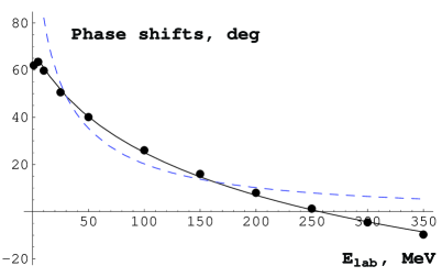
Figure 1: Phase shifts for proton-neutron scattering as a function of the laboratory energy for the ${}^{1}S_{0}$ channel. Experimental data from [8] are shown by points. The results of the calculation with the generalized interaction operator (24) are represented by the solid curve. Also given for the sake of comparison are the results of the calculation with the Yamaguchi potential (dashed curve).

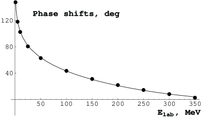
Figure 2: Phase shifts for proton-neutron scattering as a function of the laboratory energy for the ${}^{3}S_{1}$ channel. Experimental data from [8] are shown by points. The results of the calculation with the generalized interaction operator (24) are represented by the solid curve.

Thus, the following condition must be satisfied:

$$\lambda_{\varepsilon}^{-1}=J_{\varepsilon}(E_{B}).$$ (31)

The substitution of (29) into (28) then yields

$$[t_{\varepsilon}(z)]^{-1}=J_{\varepsilon}(E_{B})-J_{\varepsilon}(z)=$$

$$=(z-E_{B})\int d^{3-\varepsilon}k\frac{|\psi({\bf{k}})|^{2}}{(z-E_{k})(E_{B}-E_{k})}.$$

It can easily be proven that, upon going over to the limit $\varepsilon\rightarrow 0$ in this expression, we arrive at formula (23), which was previously obtained for the $T$ matrix; that is, the above renormalization procedure leads to the dynamics described by the interaction that is specified by Eq. (24) and which is nonlocal in time. Let us now consider this situation from the point of view of Hamiltonian dynamics. In the limit $\varepsilon\rightarrow 0$, the renormalized coupling constant $\lambda_{\varepsilon}$ and, hence, the renormalized Hamiltonian tend to zero, while the $T$ matrix (25) does not satisfy the Lippmann-Schwinger equation; therefore, the dynamics in question is not described by the Schrödinger equation. Thus, we see that, although each of the set of dynamics that correspond to the dimensionality ${\cal D}=3-\varepsilon$ for $\varepsilon>0$ is a Hamiltonian dynamics, we have a non-Hamiltonian dynamics in the limiting case ${\cal D}=3$. This situation is typical of any theory where a renormalization procedure is required to remove ultraviolet divergences. At the same time, the $T$ matrix satisfies Eq. (7), which one of the possible forms of the master dynamical Eq. (4) of generalized quantum dynamics. But Eq. (7) reduces to Lippmann-Schwinger equation only in the particular case where $H_{int}(t_{2},t_{1})$ has the form (11)- that is, in the case of an instantaneous interaction. The dynamics of a renormalized theory is nonlocal in time; that is, it belongs to the class of dynamics that can be described only on the basis of generalized quantum dynamics. For the renormalized model considered here, the generalized interaction operator is given by (24). This operator can then be used in a dynamical equation to describe the dynamics of systems featuring an arbitrary number of nucleons.

Table 1: The parameters of the interaction operator obtained by fitting the $NN$ date, $\rho=1MeV^{-1}$.

partial wave	$\alpha$	$\lambda$	$b\cdot\rho$	$d\cdot\rho$	$b_{2}\cdot\rho^{1-2\alpha}$
${}^{3}S_{1}($np$)$	0.499	$133.5\times 10^{2}$	433.8	$766.2$	$1.696\times 10^{-7}$
${}^{1}S_{0}($np$)$	0.499	131.8	356.3	$3.651\times 10^{6}$	$1.694\times 10^{-7}$
${}^{1}S_{0}($pp$)$	0.499	320.0	371.7	$6.763\times 10^{5}$	$1.695\times 10^{-7}$

IV Anomalous off-shell behavior of two-nucleon amplitudes

Thus, we have shown that the regularization of the Schrödinger and Lippmann-Schwinger equations, which is necessary in using effective interaction operators constructed within effective field theories results in that the interaction generating nucleon dynamics appears to be nonlocal in time. The evolution of systems governed by such interactions is described in a natural way, by generalized quantum dynamics and by models constructed on its basis [4,5]. In [5], the $NN$ interaction was described on the basis of the model where the generalized interaction operator has the form (24) with form factor $\psi({\bf p})=g_{Y}({\bf p})-\phi({\bf p})$, where $g_{Y}({\bf p})$ is the Yamaguchi form factor [7], which, in the S channel, is given by $g_{Y}({\bf p})=\frac{\lambda}{b^{2}+p^{2}}$, and $\phi({\bf p})=\left(d^{2}+p^{2}\right)^{-\frac{\alpha}{2}}$ with $-\frac{1}{2}<\alpha<\frac{1}{2}$; that is, $\phi({\bf p})$ is the form factor whose ultraviolet behavior corresponds to an interaction that is nonlocal in time. The parameters of the model were determined from the best fit to the experimental values [8] of the phase shift for nucleon-nucleon scattering at low energies. For the ${}^{1}S_{0}$ and the ${}^{3}S_{1}$ channel, the quality of our fits to the experimental values of the phase shifts for nucleon-nucleon scattering are illustrated in Figs. 1-3. The parameters of the model are quoted in the table. For the sake of comparison, the energy dependence of the phase shift for nucleon-nucleon scattering is also displayed in Fig. 1. From this figure, it can be seen that, in the Yamaguchi model, the main flaw, which consists in its inability to reproduce the reversal of the sign of the phase shift in the ${}^{1}S_{0}$ channel can be removed by generalizing this model to the case where the interaction is nonlocal in time.

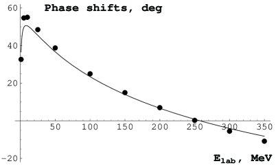
Figure 3: Phase shifts for proton-proton scattering as a function of the laboratory energy for the ${}^{1}S_{0}$ channel. Experimental data from [8] are shown by points. The results of the calculation with the generalized interaction operator (24) are represented by the solid curve.

Needless, to say, the $NN$-interaction potential constructed in this study is nothing but a model-dependent quantity. A realistic effective $NN$-interaction operator that takes into account QCD symmetries must be derived within an effective field theory by using a renormalization procedures. However, our exactly solvable model can be employed the study the effect of the nonlocality of $NN$ interaction on the character of nucleon dynamics. Among data from two-nucleon physics, information about the off-shell of two-nucleon amplitudes is of great importance, since it substantially affects the dynamics of three-nucleon and multinucleon systems [9]. Let us consider the effect of nonlocality of the $NN$ interaction on this behavior of two-nucleon amplitudes. First of all, we consider the behavior of $f(z)=\langle{\bf p}_{2}|T(z)|{\bf p}_{1}\rangle$ as a function $z$ at fixed ${\bf p}_{1}$ and ${\bf p}_{2}$. It is well known that, for $|z|\to\infty$, the solutions $\langle{\bf p}_{2}|T(z)|{\bf p}_{1}\rangle$ to the Lippmann-Schwinger equation tend to $\langle{\bf p}_{2}|V|{\bf p}_{1}\rangle$, where $V$ is the potential. Thus, we see that, in the case where the $NN$ interaction is described by some potential-that is, this interaction is local in time - the two-nucleon amplitude $\langle{\bf p}_{2}|T(z)|{\bf p}_{1}\rangle$ fends to a nonzero constant for $|z|\to\infty$. At the same time, $\langle{\bf p}_{2}|T(z)|{\bf p}_{1}\rangle$ taken at fixed ${\bf p}_{1}$ and ${\bf p}_{2}$ always tends to zero for $|z|\to\infty$ in the case of an interaction that is nonlocal in time. Indeed, we have already indicated that, in the nonlocal case, $H_{int}^{(s)}(\tau)$ does not have a delta-function singularity at the point $\tau=0$, whence one can immediately conclude that $B(z)$, which is defined by the relation (10), tends to zero for $|z|\to\infty$. According to (9), it immediately follows that, in this limit, $\langle{\bf p}_{2}|T(z)|{\bf p}_{1}\rangle$ also tends to zero. For our nonlocal model, as well as for Yamaguchi model, Fig. 4 illustrates the behavior of the function $f(z)$ in the ${}^{3}S_{1}(np)$ channel. It is obvious that this anomalous behavior of two-nucleon amplitudes, which is due to the nonlocality of the $NN$ interaction in time, can significantly affect the dynamics of multinucleon systems.

As was shown above, the generalized interaction operator can be nonlocal in time only if its matrix elements $\langle{\bf p}_{2}|H_{int}^{(s)}(\tau)|{\bf p}_{1}\rangle$ as functions of momenta have an ultraviolet behavior that leads to divergences in Hamiltonian dynamics. Accordingly, the $T$-matrix elements $\langle{\bf p}_{2}|T(z)|{\bf p}_{1}\rangle$ as functions of ${\bf p}_{1}$ and ${\bf p}_{2}$ will not decrease at infinity as fast as is required in Hamiltonian dynamics. This brings about the question of how this circumstance can affect the character of nucleon dynamics. The importance of the off-shell behavior of the two-nucleon $T$ matrix is associated with the fact that it appears in the Faddeev equation, which makes it possible to determine the $T$ matrix for the system of three nucleons if the two-nucleon $T$ matrix is known. It can straightforwardly be shown, however, that, if $\langle{\bf p}_{2}|T(z)|{\bf p}_{1}\rangle$ does not decrease sufficiently fast in the high-momentum limit, then the Schmidt norm for the kernel of the Faddeev equation does not exist at any value of $z$. Thus, we see that, in the case of an interaction that is nonlocal in time, the off-shell behavior of two-nucleon amplitudes is anomalous, which results in that the Faddeev equation is not well-defined. That effective field theories lead to a Faddeev equation whose kernel decrease at infinity insufficiently fast for this equation to be well-defined is one of the most serious problems in such theories [6]. It is important that within generalized quantum dynamics the Faddeev equation, as well as the Lippmann-Schwinger equation, need not be valid, as this does indeed occur in the case of a nonlocal interaction. One must then directly use the dynamical Eq. (4) or (7).

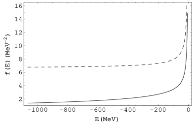
Figure 4: The off-shell behavior of $f(E)=10^{9}\langle{\bf p}|T(z)|{\bf p}\rangle,$ $|{\bf p}|=500$ MeV in the ${}^{3}S_{1}$ channel for $np$ scattering. The solid curves corresponds to the model with generalized interaction operator (24), compared to the model with Yamaguchi potential with parameters given in Yam (dashed line).

In our above analysis, we have considered the case where the interaction is nonlocal in time and is described by the interaction operator in the form (24). At the same time, it was shown in [5] that the generalized interaction operator may have the form

$$H_{int}(t_{2},t_{1})=H_{non}(t_{2},t_{1})$$

$$-2i\delta(t_{2}-t_{1})H_{I}(t_{1}),$$ (32)

where the first term on the right-hand side, $H_{non}(t_{2},t_{1})$, describes the nonlocal part of the interaction, while the second part describes its instantaneous part. This form of the interaction operator seems natural in the case of $NN$ interactions. Indeed, it is well known that, at long and intermediate distances, the $NN$ interaction is well approximated by realistic $NN$ potentials based on the concept of meson exchange. This part of the $NN$ interaction is described by the second term on the right-hand side of (30). At the same time, there is every reason to believe that a nonlocal interaction operator offers a natural way to treat the short-range part of the interaction, where quark and gluon degrees of freedom are expected to manifest themselves. From the above analysis, it follows that the asymptotic high-momentum behavior of the matrix elements $\langle{\bf p}_{2}|H_{int}(t_{2},t_{1})|{\bf p}_{1}\rangle$ of the interaction operator (30) is controlled by the nonlocal term $H_{non}(t_{2},t_{1})$. Even if this term makes a negligible contribution to two-nucleon phase shifts at low energies, it changes qualitatively the off-shell behavior of two-nucleon amplitudes and, hence, affects substantially three-nucleon data. The highlights the importance of taking into account nonlocality effects in describing the short-range part of the $NN$ interaction. The use of nonlocal interaction operators for the short-range part of the $NN$ interaction, along with realistic $NN$ employed at present, may lead to a better description of three-nucleon and multinucleon data. We hope that it will be possible to construct such operators - that is, those nonlocal interaction operators that would describe the short-range part of the $NN$ interaction - on the basis of effective field theories.

V Conclusion

By considering the example solvable model, we have shown that, upon the application of regularization and renormalization procedures, the dynamics of a nucleon system governed by an interaction that involves ultraviolet divergences is not Hamiltonian - it is described by the dynamical Eq. (4) featuring a generalized interaction operator that is nonlocal in time. Here, we are dealing with dynamics that can be consistently described only within generalized quantum dynamics. Thus, generalized quantum dynamics opens new possibilities for solving problems associated with the fact that effective field theories lead to effective nucleon-nucleon interaction operators involving ultraviolet divergences. It can be expected that nucleon dynamics to which effective field theories must lead will be described by some generalized interaction operator that is nonlocal in time. If, within an effective field theory, one will be able to construct such an operator, which will then respect QCD symmetries, it will be possible to use Eq. (4) to describe nucleon dynamics. For the example of the aforementioned model, we have shown that such an operator can be constructed. We have investigated the effect of the nonlocality of $NN$ interaction in time on the character of nucleon dynamics. Our analysis has revealed that these effects lead to an anomalous off-shell behavior of two-nucleon amplitudes: The two-nucleon amplitudes $\langle{\bf p}_{2}|T(z)|{\bf p}_{1}\rangle$ at fixed momenta vanish for $|z|\to\infty$ and, treated as functions of ${\bf p}_{1}$ and ${\bf p}_{2}$, decrease insufficiently fast at infinity for the Faddeev equation to be well-defined. This may substantially affect the dynamics of multinucleon systems. As we have shown, the nonlocal interaction operator constructed here can be used for the nonlocal part of the $NN$-interaction operator. At the same time, realistic $NN$ potentials can be taken for its instantaneous part describing the $NN$ interaction at intermediate and long distances. The introduction of such nonlocal corrections to realistic $NN$ potentials may significantly improve the description of three-nucleon and multinucleon data, which is one of the challenging problems in nucleon physics.

References

- (1) S. Weinberg, Phys. Let. B 251, 288 (1990); Nucl. Phys. B 363, 3 (1991); Ordonez C. and van Kolck U., Phys. Let. B 291, 459 (1992); Ordonez C., Ray L. and van Kolck U., Phys. Rev. Let. 72, 1982 (1994); Phys. Rev. C 53, 2086 (1996); van Kolck U., Phys. Rev. C 49 2932 (1994).
- (2) Yu.S. Kalashnikova, I.M.Narodetsky, and V.P.Yurov, Yad. Fiz., 49, 232 (1989); Yu.A.Simonov, Phys. Lett. B 107, 1 (1981); A.G. Baryshnikov, L.D.Blokhintsev, I.M.Narodetsky, and D.A.Savin, Yad. Fiz. 48, 1273 (1988); A.N. Safronov, Teor. Mat. Fiz. 89, 420 (1991); Yad. Fiz., 57, 208 (1994); Yu.A. Kuperin, K.A. Makarov, and S.P.Merkuriev, Teor.Mat.Fiz., 75, 431 (1988); 76, 242 (1989); A. Abdurakhmanov and A.L. Zubarev, Z.Phys. A322, 523 (1985); M. Orlowski, Helv.Phys.Acta. 56, 1053 (1983); B.O. Kerbikov, Yad. Fiz. 41, 725 (1985); Teor. Mat. Fiz. 65, 379 (1985).
- (3) R.Kh. Gainutdinov, J. Phys. A 32, 5657 (1999).
- (4) R.Kh. Gainutdinov and A.A. Mutygullina, Yad. Fiz. 60, 938 (1997).
- (5) R.Kh. Gainutdinov and A.A. Mutygullina, Yad. Fiz. 62, 2061 (1999).
- (6) D.R. Phillips, I.R. Afnan, and A.G. Henry-Edwards, Phys. Rev. C. 61, 044002-1 (2000).
- (7) Y.Yamaguchi, Phys. Rev. 95, 1635 (1954).
- (8) V.G.J. Stoks, R.A.M. Klomp, M.C.M. Rentmeester, and J.J. de Swart, Phys. Rev. C 48, 792 (1993).
- (9) R. Machleidt, F. Sammarruca, and Y. Song, Phys. Rev. C 53, 1483 (1996); A. D. Lahiff and I. R. Afnan, Phys. Rev. C 56, 2387 (1997).