Recent Developments in the
Nuclear Many-Body Problem

Abstract

The study of quantum chromodynamics (QCD) over the past quarter century has had relatively little impact on the traditional approach to the low-energy nuclear many-body problem. Recent developments are changing this situation. New experimental capabilities and theoretical approaches are opening windows into the richness of many-body phenomena in QCD. A common theme is the use of effective field theory (EFT) methods, which exploit the separation of scales in physical systems. At low energies, effective field theory can explain how existing phenomenology emerges from QCD and how to refine it systematically. More generally, the application of EFT methods to many-body problems promises insight into the analytic structure of observables, the identification of new expansion parameters, and a consistent organization of many-body corrections, with reliable error estimates.

1 Introduction

At a fundamental level, atomic nuclei are described by quantum chromodynamics (QCD) with colored quark and gluon degrees of freedom, whose interactions are asymptotically free at short distances. Yet under ordinary conditions, colorless nucleons in a nucleus largely retain their identity [1]. In the traditional approach to the low-energy nuclear many-body problem, a phenomenological two-nucleon potential is fit to scattering data and properties of the deuteron, and solutions to the many-body Schrödinger equation for nuclei across the periodic table and nuclear matter are approximated by various sophisticated methods. Three-body forces and meson-exchange currents are added only when required by discrepancies with data. The study and validation of QCD in other contexts over the past quarter century has had relatively little impact on this phenomenology [1].

Recent developments are changing this situation in two major ways. First, the nuclear many-body problem has become the QCD many-body problem, involving explorations of phenomena throughout the phase diagram of QCD. Second, effective field theory (EFT) methods are being used to build bridges from QCD to traditional nuclear many-body phenomenology. The phrase “effective theory” has often denoted a model used because one couldn’t solve the underlying theory. In contrast, an EFT is a field theory that reproduces the results of an underlying theory in a systematic and model-independent way, but in a limited domain.

It would be impractical to make a complete survey of this broad range of activity, so we will instead present a coarse-grained tour with selected stops. Many more details are available in the cited references. We will start with “teasers” from two of the many new frontiers in exploring the QCD phase diagram, many-body physics at small $x$ and color superconductivity. New insights into established approaches within the traditional framework and how successful phenomenology emerges from low-energy QCD are considered next. Finally, we give an example of how new ideas for attacking many-body problems arise from applying the EFT perspective.

2 Exploring the QCD Phase Diagram

Quantum chromodynamics (QCD) is a gauge theory of SU(3) color charges, with quarks and gluons as the fundamental degrees of freedom. It has many analogies to quantum electrodynamics (QED), but important differences follow from the non-abelian structure. In particular, gluons carry the color charge and interact with each other. Two prominent consequences are asymptotic freedom (the interaction becomes weak at high energies/short distances) and color confinement (observed hadrons have no net color charge). Quarks come in six varieties, called flavors, with masses that are very small compared to the relevant QCD scale (up, down) or very large (charm, top, bottom). The strange quark mass is somewhere in the middle; whether it should be considered heavy or light has an important influence on the phase structure of QCD.

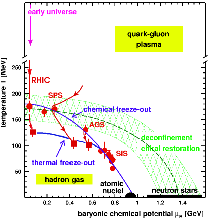
Figure 1: The conjectured phase diagram of QCD (see Ref. HEINZ for details).

Figure 1 is a conjectured phase diagram for QCD. The axes here are the temperature and the chemical potential for baryon number. The traditional nuclear many-body problem lives in the small black blob at low temperature with chemical potential near one GeV. But now the nuclear many-body problem encompasses the entire plane and can more correctly be termed the QCD many-body problem. Even the physical vacuum ($T=0$, $\mu_{B}=0$) is an extraordinarily complex, coherent many-body medium characterized by nonperturbative quark and gluon condensates [2].

One of the main tasks of the new nuclear many-body problem is to explore the phase structure in Fig. 1, such as the expected deconfinement and chiral symmetry restoration phase transitions. These transitions are predicted by lattice simulations; however, the simulations are restricted at present to zero chemical potential. Energetic collisions of heavy nuclei are being used to probe different regions of temperature and chemical potential; the figure shows data points from several heavy-ion experiments. The latest accelerator, RHIC, is now running and producing data [2, 3].

There are many interesting challenges for many-body theory implicit in Fig. 1. Here we will briefly consider only two: small-$x$ physics and color superconductivity.

2.1 Many-Body Physics at Small $x$

The initial conditions of ultra-relativistic heavy-ion collisions strongly influence the details of quark-gluon plasma formation. Particularly important are the “wee” parton distributions in nuclei, which are virtual excitations of the nuclear ground state (mostly gluons) carrying a small fraction $x$ of the longitudinal momentum of each colliding nucleus [4]. Large energy $s$ and momentum transfer $Q^{2}$ but small $x\propto Q^{2}/s$ is the regime of high virtual gluon densities. Perturbative QCD evolution predicts rapid growth in the gluon distribution as $x\rightarrow 0$, but eventually gluon recombination and screening effects should become important. An important question is whether the gluon density saturates and at what scale [4].

The large occupation number of gluon states implies that a classical effective field theory (EFT) is a good starting point, with corrections from a nonlinear renormalization group analysis. The characteristic energy scale at RHIC and planned future accelerators is high enough that the effective coupling is weak, although the physics is nonperturbative. McLerran and collaborators have predicted Bose-Einstein condensation at sufficiently high gluon density, leading to a new state of matter they call a “colored glass condensate.” With respect to natural time scales, the color fields evolve slowly and are disordered[5, 6]. The EFT for this system, formulated in the infinite momentum frame (in light cone gauge) is a (nearly) two-dimensional theory with a structure mathematically analogous to that of a disordered system of Ising spins in a random magnetic field [5]. Over the coming decade, ongoing work on the theory of high density QCD will elucidate experimental signatures of this condensate [2].

2.2 Color Superconductivity

Could the interior of a neutron star be a quark-gluon fluid, as implied by Fig. 1? It would seem so based on a naive argument: asymptotic freedom implies that the force between quarks weakens as the momentum scale of interaction increases, and the behavior at low temperature and high density is determined by high-momentum quarks at the Fermi surface, so we would expect matter to be a Fermi sea of essentially free quarks. However, this argument is well known to be too naive: if there is quark-quark attraction, then a Cooper pairing instability is inevitable. In fact, an analysis using one-gluon-exchange (applicable at very high density) or instanton-induced interactions (nonperturbative effects at lower density) indicate attraction between quarks in the color anti-symmetric $\overline{3}$ state [7, 8, 9].

The methods of superconductivity have been readily adapted to this problem, which has drawn particular interest because this high density regime is theoretically tractable. There is a rich and structured theory revealed as one varies the number of colors $N_{C}$ and the number of quark flavors $N_{f}$ (and their masses). To assess the different possible instabilities, theorists have studied the renormalization-group evolution of four-fermion operators using the methods pioneered by Shankar and Polchinski [10], in which one integrates out states toward the Fermi surface. The central result of the analysis is the identification of condensates in diquark channels, analogous to Cooper pairs of electrons; this is called color superconductivity [8].

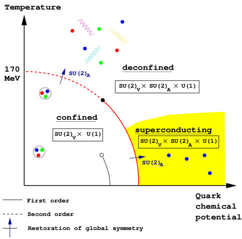
Figure 2: Phase diagram for two massless flavors [9].

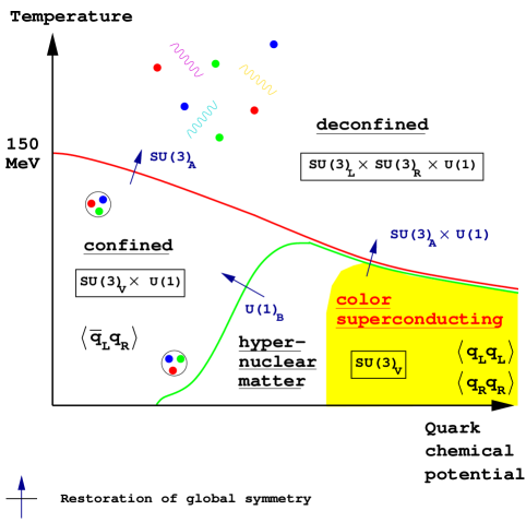
Figure 3: Phase diagram for three massless flavors [9].

To determine how the instability is resolved, a model energy functional for the ground state is needed. The simplest analyses use four-Fermi interactions in a self-consistent mean-field (NJL) gap equation. In the vacuum, a non-trivial solution gives a constituent mass for quarks from spontaneous chiral symmetry breaking; calibrating this to be about 400 MeV determines the coupling. Then one studies the quantitative phase structure [9].

For two massless flavors (so $m_{s}\rightarrow\infty$), the color $\overline{3}$, flavor singlet channel wins, and $SU(3)_{\rm color}$ is broken down to $SU(2)_{\rm color}$. The phase and symmetry structure is illustrated in Fig. 2. The low-lying spectrum has five massive gluons and two colored massive quarks with gap $\Delta$. There is a tri-critical point that survives the small up/down quark masses, which may be observable in heavy-ion collisions as the analog of critical opalescence [8].

For three massless flavors, the preferred mode is “color flavor locking,” which implies color and flavor are each broken, but combinations of generators remain good symmetries. There are eight massive gluons and all quark modes are gapped. The phase and symmetry structure is illustrated in Fig. 3. A fascinating possibility is quark-hadron continuity: that these excitations map smoothly onto the hadronic phase. For example, the gluons become the octet of vector bosons in hypernuclear matter. A current challenge is to determine the correct interpolation of these phases for real-world quark masses.

All analyses have revealed truly high-$T_{c}$ superconductors, with gaps of order 100 MeV (with current uncertainties plus or minus a factor of two) and critical temperatures of order 50 MeV or $10^{12}\,$K. Since the attractive force comes from a primary interaction, color superconductivity is particularly robust. The temperature in a neutron star after a few seconds following its birth is much less than the critical temperature, so if the interior density is high enough to support quark matter, it will be a color superconductor.

Detecting the consequences of color superconductivity for neutron star physics is a challenge, however. The impact on the equation of state is ${\cal O}(\Delta/\mu)^{2}$, which at a few percent is much less than the uncertainties in the equation of state. Thus the main signatures will be found elsewhere. Since color superconductivity gives mass to low-lying excitations, one should look toward transport phenomena (mean-free paths, conductivities, viscosities, and the like). One proposal is that the cooling rate of neutron stars, which is determined by the heat capacity and emissivity, should show a characteristic slow-down signature for the 2SC phase. The color-flavor locking phase might be detected by the time distribution of the neutrino pulse from a supernova (such as 1987A). Future work will concentrate on sharpening these signals and exploring other possibilities [8].

3 From QCD to Nuclear Phenomenology

How does traditional nuclear phenomenology relate to QCD? Proposed paths from low-energy QCD to nuclei have included models with explicit constituent quark degrees of freedom (e.g., a quark shell model) and many-body skyrmions, in which nucleons appear as solitons in the pion field. However, these approaches have had little quantitative impact on our understanding of nuclear many-body physics and little qualitative relation to the traditional approach. In recent years a much more promising candidate has emerged: chiral effective field theory.

3.1 Chiral Effective Field Theory

The effective field theory approach is grounded in some very general physical principles [11]. If a system is probed or interacts at low energies, resolution is also low, and fine details of what happens at short distances or in high-energy intermediate states are not resolved. Therefore, the short-distance structure can be replaced by something simpler without distorting the low-energy observables. This is analogous to a multipole expansion, in which a complicated, distributed charge or current distribution is replaced for long-wavelength probes by a series of point multipoles. The use of a local lagrangian provides a framework for carrying out this program in a complete and systematic way. The uncertainty principle implies that high-energy intermediate states are highly virtual and only last for a short time, so their effects are not distinguishable from those of local operators [11].

The effective degrees of freedom (dof’s) depend on a separation or resolution momentum scale $\Lambda$. Long-range dof’s must be treated explicitly while short-range physics is encoded in the coefficients of the local operators. For low-energy QCD at the momentum scales relevant for bound nucleons, the appropriate degrees of freedom (neglecting strangeness) are pions and nucleons, and $\Lambda\approx 500$–$1000\,$MeV. The long-range pion physics is constrained by chiral symmetry, so we have a chiral EFT, which has much in common with traditional potential models [1].

There are three general ingredients of an EFT approach, which we will illustrate with the particular details of the chiral EFT. Further explanations and other examples can be found in Ref. CROSSING.

1. Construct the most general lagrangian density with appropriate low-energy degrees of freedom that is consistent with the global and local symmetries of the underlying theory. For chiral EFT, this means ${\cal L}_{\rm eft}={\cal L}_{\pi\pi}+{\cal L}_{\pi N}+{\cal L}_{NN}$, so nuclear many-body physics is united with pion-pion and pion-nucleon scattering physics. Chiral symmetry allows us to treat long-distance pion physics systematically.

2. The declaration of a regularization and renormalization scheme. Because the long-distance physics is insensitive to details of short-distance physics, the results are ultimately independent of the details of the scheme, but different approaches may have different convergence properties. Also, the most useful EFT formulation will depend on the few- or many-body system under consideration. The most advanced chiral EFT calculations at present use a smooth momentum cutoff [12].

3. A well-defined power counting, which provides small expansion parameters. Power counting is a procedure to determine what graphs to include (or sum) at each order. It ensures consistency with physical principles and conservation laws while allowing estimates of truncation errors. The separation of physical scales provides expansion parameters; for chiral EFT it is the momentum ${\bf p}$ and/or pion mass $m_{\pi}$ (generically called $Q$) divided by a chiral symmetry breaking scale $\Lambda_{\chi}\approx 1\,$GeV. Weinberg’s prescription is to power count the effective potential $V_{NN}$ and then solve the Schrödinger equation. Chiral symmetry implies $V_{NN}=\sum_{\nu=\nu_{\rm min}}^{\infty}c_{\nu}Q^{\nu}$, where $\nu$ is given by a formula based on the topology of a given diagram and the nature of its vertices. The key to a systematic expansion is a lower bound $\nu_{\rm min}$ [13].

Figure 4: NN phase shift predictions in LO (dots), NLO (dashes), and NNLO (solid) compared to experiment (diamonds). The $x$–axis is the energy in GeV and the $y$ axis is in degrees.

The most complete application of this framework has been by Epelbaum et al., who have adapted a unitary transformation method to obtain an energy-independent potential [12]. Their recent results reveal an orderly progression in predictions from LO to NLO to NNLO (next-to-next-to-leading order), as shown for two (of many) neutron-proton scattering phase shifts in Fig. 4 [12]. At each order, the power counting scheme specifies the new diagrams needed; coefficients are determined from fits to $\pi N$ or $NN$ scattering data at low energy. The calculations become closer to experiment (better at low energy) and less sensitive to the value of the momentum cutoff (which is 500–600 MeV for NNLO), in accord with the expectations of an EFT.

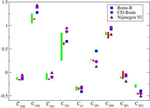
Figure 5: Comparing coefficients from phenomenological models to chiral EFT [12]. The leftmost bar for each coefficient is LO (the length reflects the variation with cutoff), the middle bar is NLO, and the symbols are values extracted from the indicated boson-exchange potentials.

The coefficients in the lagrangian can be estimated by naive dimensional analysis (NDA), as originally proposed for low-energy QCD by Georgi and Manohar. Any term in the lagrangian with nucleon fields $N$ and pion fields $\pi$ can be put in the form:

$${\cal L}_{\rm eft}\sim c_{lmn}\left(\frac{N^{\dagger}(\cdots)N}{f_{\pi}^{2}\Lambda_{\chi}}\right)^{l}\left(\frac{\pi}{f_{\pi}}\right)^{m}\left(\frac{\partial^{\mu},m_{\pi}}{\Lambda_{\chi}}\right)^{n}f_{\pi}^{2}\Lambda_{\chi}^{2}\ ,$$ (1)

where the pion decay constant $f_{\pi}\approx 100\,$MeV and the chiral symmetry breaking scale $\Lambda_{\chi}\approx 1000\,$MeV. If these scales are correctly incorporated, the remaining dimensionless couplings $c_{lmn}$ should be of order unity; if so they are called “natural”. The explicit fits verify that the EFT is natural except for one combination of constants that is unnaturally small. This is a signature of a symmetry not explicitly considered; in this case it is the Wigner $SU(4)$ spin-isospin symmetry [12].

The constants also reveal that the chiral EFT potential is closely related to conventional NN potentials based on boson exchange. The latter can be considered to be models of the short-distance physics that is unresolved in the chiral EFT (except for pion exchange). Therefore, this physics should be encoded in the coefficients of contact terms in the EFT. We can test this relation by comparing the chiral EFT coefficients to corresponding coefficients derived from several boson-exchange models in Fig. 5. The pattern from the chiral EFT is a blueprint of low-energy QCD and it is quantitatively reproduced by the phenomenology [12]. This is a major step towards the construction of a path from QCD to the inputs of traditional nuclear many-body theory!

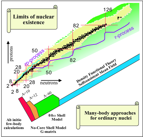
Figure 6: Table of nuclides and corresponding theoretical approaches for different regimes of nucleon number $A$ [14].

The theoretical many-body approaches for nuclei under ordinary conditions are shown in Fig. 6. For low $A$ (total number of protons plus neutrons), Monte Carlo methods are able to calculate directly given free-space potentials. In the intermediate region shell-model methods are used, while in the region of large $A$, where most of the nuclides lie, self-consistent mean-field models and related approaches are most often applied. We consider the impact of EFT approaches on each in turn.

3.2 Monte Carlo calculations of Light Nuclei

Nuclei present a spin-isospin nightmare that make the cost of direct Monte Carlo calculations grow exponentially with $A$. Through heroic efforts, Carlson et al. have recently pushed Green’s function Monte Carlo (GFMC) methods through $A=10$ with an accuracy in binding energies of 1% or better;[15] the practical limit with current algorithms is probably $A\approx 12$.

The significance of 1% calculations is that nuclear forces can be unambiguously tested. An important result is seen by comparing experimental spectra to predictions generated using only the two-body potential (see Fig. 7) [15]. The predictions are underbound and the absolute shortfall grows with $A$, making many-body forces not only inevitable but quantitatively critical. Further, a particular isospin dependence from three-nucleon forces (3NF) is needed and 1/2 to 2/3 of the spin-orbit splittings come from three-body forces. Currently a semi-phenomenological form is fit to $A\leq 8$ energy levels, but there is a basic problem: the number of possible operators for 3NF is much larger than for NN and it is not practical to examine them all.

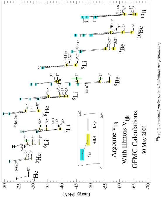
Figure 7: Energy spectra in nuclei up to $A=10$ [15]. In each set of levels, calculations with only the two-body Argonne $V_{18}$ potential are on the left and those with a semi-phenomenological three-body force included are in the middle. Experimental levels are on the right.

Chiral EFT comes to the rescue with a systematic power-counting scheme that predicts the hierarchy of many-body forces as well as the hierarchy for different three-body forces [13]. As with two-body forces, at each order in the EFT expansion the power counting scheme specifies the additional three-body diagrams that should be included. Coefficients of purely short-range three-body terms must be fit to three-body scattering or bound state observables. Note that because the description is model independent, a fit to one set of observables can be applied to any other set of observables. An issue of current study (and controversy) is whether the $\Delta$ resonance should be included as a lagrangian degree of freedom [13].

The next step is to adapt the chiral EFT calculations for GFMC, which requires local versions of the EFT potential to be constructed. Then $A\geq 4$ predictions with a connection to QCD will be possible! The future of Monte Carlo for nuclei will likely be Auxiliary Field Diffusion Monte Carlo (AFMDC) with spin-dependent interactions between nucleons replaced by interactions between nucleons and auxiliary fields. The great advantage is that one can sample spins and isospins along with coordinates, so that the cost grows only as $A^{3}$; up to $A\approx 100$ may be feasible.

3.3 The Shell Model Revisited

In the conventional nuclear shell model, a given free-space Hamiltonian in the full Hilbert space ($P+Q$) is transformed to an effective Hamiltonian that is diagonalized in a truncated model space ($P$), with the same results for low-energy observables (see the left side of Fig. 8). A harmonic oscillator basis is used to separate relative and center-of-mass (COM) motion (recall that there is no fixed COM for nuclei). A similarity transformation may be used to decouple the $P$ and $Q$ space or, in practice, a phenomenological interaction might be used.

There are many problems with actual shell-model implementations, which date from an earlier era in which computational limitations necessitated severe compromises. Even if only a two-body potential is used in the $P+Q$ space, the removal of high-momentum states invariably generates many-body forces; in practice only two-body effective interactions are used. Another problem is sensitive dependence on unphysical parameters, such as the cutoff $\Lambda_{\rm SM}$ for the $P$ space or “starting energies”. Perhaps most importantly, not only the Hamiltonian but all operators in the $P$ space must be effective operators; however, either bare operators are used or a naive and uncontrolled renormalization (e.g., multiplicative scaling) is applied.

The shell model approach is a natural setting for renormalization group methods. The first steps to take conventional nuclear models to controlled EFT counterparts have been taken recently by Haxton and collaborators [16]. They have developed a self-consistent Bloch-Horowitz approach using Lanczos methods. The Lanczos construction means that the expensive part of the calculation need only be performed once and then effective Hamiltonians and operators for each state can be generated cheaply. The importance of effective operators is illustrated by the plot on the right in Fig. 8. With bare operators, the form factor for different $P$ spaces is almost random for momentum transfers above 2 fm^-1, while even at low momentum the renormalization is clearly not a simple scaling, as is often assumed. In contrast, if effective operators are used, results are independent of the truncation of the space.

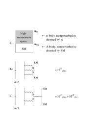
Figure 8: On the left is a schematic representation of full and shell model (SM) spaces. The $P$ space is up to $\Lambda_{\rm SM}$ and the $Q$ space is from $\Lambda_{\rm SM}$ to $\Lambda_{\infty}$. On the right is the magnetic dipole $M1$ form factor for ³He calculated in the full space and with bare operators in various truncated spaces [16]. The curves using effective operators for the same spaces are indistinguishable from the full (solid) curve.

   

To extend the Bloch-Horowitz approach to heavier nuclei, it is necessary to effectively decrease the upper bound used to define the full space, $\Lambda_{\infty}$. One might hope that perturbation theory could be used to include the effect of higher energy states. Even the simplest calculation (e.g., the binding energy of the deuteron) shows that the nonperturbative effects of the hard-core repulsion in typical NN potentials spoils any hope of rapid convergence [16]. However, according to the EFT precepts, the singular contributions from the potential are not resolved in the low-energy shell-model space, so we can replace them by something simpler: separable contact interactions and derivatives. In practice this leads to an expansion of the harmonic oscillator matrix elements (Talmi integrals) in powers of the hard core radius over the oscillator potential [16].

This expansion is matched in the full space and the coefficients obtained can then be evolved to lower $\Lambda$ analytically using a shell renormalization group equation. Perturbation theory can be used on the remaining soft potential; convergence at leading order is rapid [16]. Currently various details of the NLO implementation and beyond are being worked out, and then the formalism will be embedded in heavier nuclei. Eventually the starting potential in the $\Lambda_{\infty}$ space may be taken from the chiral EFT, furthering the connection to QCD.

3.4 Power Counting for Density Functionals

The large-$A$ region of the table of nuclides requires a different plan of attack. The most widely used approaches are referred to as “self-consistent mean field” calculations, but this is a misleading nomenclature, which implies a Hartree or Hartree-Fock calculation of some underlying interaction. In fact, it is more appropriate to identify these calculations as Kohn-Sham density functional theory (DFT), in which the full Hartree plus exchange-correlation functionals (and not Hartree alone!) are approximated by a parametrized form. “Mean field” in this context really means a limited form of the analytic and nonlocal structure in the energy functional.

The role of EFT methods here starts with a power counting for Skyrme or covariant energy functionals. We consider Skyrme-type functionals here; the case of covariant functionals is addressed in Brian Serot’s talk [17]. The functional (given here for $N=Z$ only) is built from densities ($\rho$), kinetic energy densities ($\tau$), and currents (${\bf J}$), all obtained as sums over occupied Kohn-Sham single-particle wave functions: [18]

$$\epsilon[\rho,\tau,{\bf J}] = {1\over 2M}\tau+{3\over 8}t_{0}\rho^{2}+{1\over 16}t_{3}\rho^{3}+{1\over 16}(3t_{1}+5t_{2})\rho\tau$$ (2)

$$\hbox{}+{1\over 64}(9t_{1}-5t_{2})(\nabla\rho)^{2}-{3\over 4}W_{0}\rho\nabla\cdot{\bf J}+{1\over 32}(t_{1}-t_{2}){\bf J}^{2}\ ,$$

with typical [e.g., SkIII] model parameters (in conventional units): $t_{0}=-1129$, $t_{1}=395$, $t_{2}=-95$, $t_{3}=14000$, and $W_{0}=120$ [18]. Such large and unsystematic values imply that errors from omitted terms may be uncontrolled.

However, after applying the same Georgi-Manohar NDA that accounts for the chiral EFT coefficients [Eq. (1)], we obtain the scaled energy functional: [19]

$$\epsilon[\rho,\tau,{\bf J}] = {\tau\over\Lambda}\Bigl{(}c_{1}+c_{4}\bar{\rho}+{c_{8}\bar{\rho}^{2}}\Bigr{)}+{\rho^{2}\over f_{\pi}^{2}}\Bigl{(}c_{2}+c_{3}\bar{\rho}+{c_{9}\bar{\rho}^{2}}\Bigr{)}$$ (3)

$$\hbox{}+{(\nabla\rho)^{2}\over f_{\pi}^{2}\Lambda^{2}}\bigl{(}c_{5}+{c_{10}\bar{\rho}}\bigr{)}+{\rho\nabla\cdot{\bf J}\over f_{\pi}^{2}\Lambda^{2}}\bigl{(}c_{6}+{c_{11}\bar{\rho}}\bigr{)}+\cdots$$

with natural coefficients: $c_{1}=0.5$, $c_{2}=-0.48$, $c_{3}=1.05$, $c_{4}=1.14$, $c_{5}=1.62$, $c_{6}=-2.31$, and $c_{7}=0.39$. The naturalness of the coefficients means that truncation errors from the next order of coefficients can be estimated reliably. Additional fits to nuclei have validated these estimates and the robustness of the power counting. Work is in progress to embed the Kohn-Sham DFT framework within an EFT framework using an effective action formalism.

The path for an ab initio QCD calculation of heavy nuclei is becoming cleared, although construction is far from complete. The key will be to obtain the coefficients for the Kohn-Sham DFT/EFT not from data but from matching to the chiral effective field theory. In turn, those coefficients will not be taken from data but calculated from matching to nonperturbative lattice QCD calculations. The latter step may seem far-fetched at this point in time, but recent work using partially quenched lattice QCD to calculate coefficients for pion chiral perturbation theory is very encouraging [20]. A compelling feature is that the matching does not have to occur for a physical experiment or indeed even for a physical situation. An example is the partially quenched lattice calculation, in which valence quark masses are different from those in the quark-antiquark sea.

4 New Ideas for Many-Body Problems

While renormalization group ideas are widespread in condensed matter many-body theory, the different flavor of EFT approaches used in particle/nuclear theory can give new insight into familiar many-body problems. The dilute fermi gas (e.g., hard sphere of radius $R$) is a case in point. What happens if we apply the EFT program?

We probe the system at low resolution ($k\ll\Lambda\equiv 1/R$), so all of the physics is short distance and we can use the analog of a multipole expansion. Thus our EFT lagrangian is the most general set of local (contact) interactions: [21]

$${\cal L}_{\rm eff} = \psi^{\dagger}\Bigl{[}i\frac{\partial}{\partial t}+\frac{\overrightarrow{\nabla}^{\,2}}{2M}\Bigr{]}\psi-\frac{{C_{0}}}{2}(\psi^{\dagger}\psi)^{2}+\frac{{C_{2}}}{16}\bigl{[}(\psi\psi)^{\dagger}(\psi\!\stackrel{{\scriptstyle\leftrightarrow}}{{\nabla}}\!{}^{2}\psi)+\mbox{ h.c.}\bigr{]}$$ (4)

$$\hbox{}+\frac{{C_{2}^{\prime}}}{8}(\psi\!\stackrel{{\scriptstyle\leftrightarrow}}{{\nabla}}\!\psi)^{\dagger}\cdot(\psi\!\stackrel{{\scriptstyle\leftrightarrow}}{{\nabla}}\!\psi)-\frac{{D_{0}}}{6}(\psi^{\dagger}\psi)^{3}+\ldots$$

There are infinitely many choices for a regularization/renormalization scheme; which should we choose?

Ideally, only the short-distance scale $\Lambda$ would be in the coefficients (besides an overall factor of the fermion mass), with no auxiliary scales. This would make dimensional analysis a powerful, predictive tool and optimize our power counting prescription. However, most regulators such as a cutoff or form factor in a model potential will introduce a cutoff scale $\Lambda_{c}$, which can appear both in the coefficients and the loop integrals. That allows arbitrary functions of the dimensionless variables $\Lambda_{c}/\Lambda$ and $k_{\scriptscriptstyle\rm F}/\Lambda_{c}$, which mean that different orders in the $k_{\scriptscriptstyle\rm F}$ expansion are mixed in any given diagram. We would like a regularization and renormalization prescription that does not introduce any new scales (except possibly in logarithms).

These conditions are satisfied by dimensional regularization and minimal subtraction (DR/MS). A simple matching to the effective range expansion for two-body scattering determines the two-body coefficients ($C_{i}$) to any desired order; three-body and higher coefficients ($D_{i}$, …) must be determined by matching to many-body observables. The consequence of this scheme at finite density are simple Hugenholtz diagrams for the energy density at $T=0$, with each diagram contributing to exactly one order in the $k_{\scriptscriptstyle\rm F}$ expansion [21]. The contribution for each diagram is a coefficient with all of the $\Lambda$ dependence times a multi-dimensional integral that is simply a geometric factor (and which is conveniently evaluated even at high order using Monte Carlo integration). The absence of an auxiliary scale $\Lambda_{c}$ means a particularly clean comparison of particle and hole contributions, which is obscured in conventional treatments [21].

Another consequence is that the renormalization group equations become a powerful tool in revealing the analytic structure of observables. It is well known that the energy density for this system has a term proportional to $k_{\scriptscriptstyle\rm F}^{9}\ln(k_{\scriptscriptstyle\rm F})$. The EFT formulation simplifies the identification and renormalization of such logarithms. The beta functions are polynomials in the couplings with $\Lambda$-independent coefficients, which means that matching powers of $\Lambda$ on either side of the renormalization group equations severely restricts the possible contributions [22]. The bottom line is that one can identify the possible powers of logarithms that occur in the energy density and the corresponding diagrams that must be inspected for log divergences (see Refs. BRAATEN and HAMMER00 for more details).

What if the problem is nonperturbative in the effective field theory couplings? (Note that even the dilute hard-sphere example is nonperturbative in the underlying interaction.) A dilute Fermi system with a large scattering length $a_{s}$ provides an illustrative example. The EFT power counting described above, when applied to the large $a_{s}$ system, implies that all diagrams with $C_{0}$ coefficients (two-body contact terms with no derivatives) must be summed (although all other contributions are perturbative). At finite density this sum is intractable, so we are led to search for an additional expansion parameter. Using DR/MS makes it transparent that we seek a geometric factor as an expansion parameter, which implies expanding in the number of space-time dimensions $D$ (actually, the expansion parameter turns out to be $1/2^{D/2}$). The expansion is detailed in Ref. STEELE00, although it has only been carried out to leading order to date.

5 Summary

The nuclear many-body problem has now expanded beyond its traditional scope to become the QCD many-body problem. Explorations of the QCD phase diagram are accelerating, with new experimental results from relativistic heavy-ion collisions and new theoretical attacks on the frontiers. Effective field theory approaches are playing a role throughout, including recent progress on the traditional problem of calculating nuclei under ordinary conditions in terms of potentials fit to two- and three-body data. Although many gaps remain to be filled, a path for ab initio calculations of heavy nuclei starting from QCD with quarks and gluons is now conceivable. More generally, the application of EFT methods to many-body problems promises insight into the analytic structure of observables, the identification of new expansion parameters, and a consistent organization of many-body corrections, with reliable error estimates.

References

- [1] S. R. Beane et al., “From Hadrons to Nuclei: Crossing the Border,” nucl-th/0008064 and references therein.
-
[2]
“High Energy Nuclear Physics,”
report from the Brookhaven National Laboratory Townmeeting,
January, 2001.
[http://www.star.bnl.gov/STAR/nsac/papers/tp.pdf] - [3] U. Heinz, “From SPS to RHIC: Breaking the Barrier to the Quark-Gluon Plasma,” to be published in the proceedings of the QCD@work conference, Martina Franca, June, 2001, hep-ph/0109006.
- [4] R. Venugopalan, Pramana 55 (2000) 73, hep-ph/0005096.
- [5] L. McLerran, hep-ph/0104285.
- [6] E. Iancu and L. McLerran, Phys. Lett. B510 (2001) 145.
- [7] D. Bailin and A. Love, Phys. Rept. 107 (1984) 325 and references therein.
- [8] K. Rajagopal and F. Wilczek, “The Condensed Matter Physics of QCD, ” hep-ph/0011333 and references therein.
- [9] M. Alford, Ann. Rev. Nucl. Part. Sci. (in press), hep-ph/0102047.
- [10] R. Shankar, Rev. Mod. Phys. 66, 129 (1993); J. Polchinski, hep-th/9210046.
- [11] G. P. Lepage, “What is Renormalization?”, in From Actions to Answers (TASI-89), edited by T. DeGrand and D. Toussaint (World Scientific, Singapore, 1989), p. 483; “How to Renormalize the Schrödinger Equation,” nucl-th/9706029.
- [12] E. Epelbaum, W. Glöckle, and U.-G. Meißner, Nucl. Phys. A671 (2000) 295; Nucl. Phys. A684 (2001) 371; nucl-th/0106007.
- [13] U. van Kolck, Prog. Part. Nucl. Phys. 43 (1999) and references therein.
-
[14]
“RIA Physics White Paper,”
report from the RIA 2000 Workshop in Durham, NC, July, 2000.
[http://www.nscl.msu.edu/conferences/riaws00/ria-whitepaper-2000.pdf] - [15] S.C. Pieper et al., Phys. Rev. C 64 (2001) 014001.
- [16] W. C. Haxton and T. Luu, Nucl. Phys. A690 (2001) 15; W. C. Haxton and C. L. Song, Phys. Rev. Lett. 84 (2000) 5454.
- [17] B. D. Serot, contribution to these proceedings.
- [18] P. Ring and P. Schuck, The Nuclear Many-Body Problem (Springer-Verlag, New York, 1980).
- [19] R. J. Furnstahl and J. C. Hackworth, Phys. Rev. C 56 (1997) 2875.
- [20] Sharpe, S. and N. Shoresh, Phys. Rev. D 62 (2001) 074505.
- [21] H.-W. Hammer and R. J. Furnstahl, Nucl. Phys. A678 (2000) 277.
- [22] E. Braaten and A. Nieto, Phys. Rev. B 55 (1997) 8090; 56 (1997) 14745.
- [23] J. Steele, Phys. Rev. Lett. (2001), in press, nucl-th/0010066.