Nucleon deformation in finite nuclei

The deformation of a nucleon embedded in various finite nuclei is considered by taking into account the distortion of the chiral profile functions under the action of an external field representing the nuclear density. The baryon charge distribution of the nucleon inside light, medium–heavy and heavy nuclei is discussed. The mass of the nucleon decreases as it is placed deeper inside the nucleus and reaches its minimum at the center of the nucleus. We discuss the quantization of non-spherical solitons and its consequences for the mass splitting of the $\Delta$ states. We show that bound nucleons acquire an intrinsic quadrupole moment due to the deformation effects. These effects are maximal for densities of nuclei about $\rho(R)\sim 0.3\div 0.35\rho(0)$. We also point out that scale changes of the electromagnetic radii can not simply be described by an overall swelling factor.

I Introduction

The possible modification of nucleon properties in the nuclear medium is currently a much discussed topic in low energy hadron physics. One way to consider such problems is to describe the nucleon as a topological soliton and then study the influence of baryonic matter on the properties of such solitons, making use of the independent particle picture which has been so successful in describing many properties of nuclei. There exist already some works where nucleons described as Skyrme–type solitons embedded in infinite nuclear matter have been considered [1, 2]. The results of these studies were in qualitative agreement with experimental indications and with results of other authors using different approaches. On the quantitative level, however, there is a too large renormalization of the nucleons’ effective mass in nuclear matter. The quantitative value of this renormalization is about $\sim 40\%$ for the normal nuclear matter density, $\rho_{0}=0.5m_{\pi}^{-3}$ [1]. It is therefore difficult to relate this modification of the nucleon self–energy in the medium to the nucleon mass in free space because such calculations consider only the special case when a nucleon is placed in the center of the heavy nucleus. The infinite nuclear matter approach allows one only to consider properties of nucleons placed near the center of heavy nuclei where the density is constant. One can expect that taking into account non-spherical effects, i.e. deformation of the skyrmion in the finite nucleus, would improve the results also on the quantitative level. Density changes play an important role when the nucleon is placed at sufficiently large distances from the center of nucleus.

The role of deformation effects (for an early work see [5]) has already been investigated in connection with the nucleon–nucleon interaction in ref. [6]. The results presented in this work demonstrated the necessity of non-spherical deformed solutions of the field equations to obtain a reliable description of the $NN$ potential. A similar approach to the deformation for two interacting skyrmions has been used in the work [7], where changes in the nucleon shape are investigated by letting the nucleon deform under the strong interactions with another nucleon. On the other hand, rotational and vibrational excitations of deformed skyrmions have also been considered for baryon number equal to one ($B=1$) system [8]. In a series of papers [9, 10, 11] axially symmetric few–skyrmion systems with baryon number $B$ larger than one were investigated, because spherically symmetric configurations in the skyrme model do not give bound skyrmionic systems [12] even for the solutions of the model within the finite nuclei as considered in ref. [13] (for similar or related work, see also ref. [14]). In the works [8, 10, 11] the deformation is introduced by a modification of the unit spherical vector and additionally through the modification of the profile function [9] in the expression of the ansatz for the chiral field (for more precise definitions, see below). The results of all investigations for $B>1$ systems lead to the conclusion that the system has to be deformed to obtain the ground state. Some other papers that deal with deformation effects and non-spherical configurations are collected in refs. [15].

In the present work we consider properties of the deformed nucleon embedded in light, medium–heavy and heavy nuclei. Deformation effects are introduced by the distortion of the profile function of chiral field under the action of the external field (which parameterizes the baryonic density within a given nucleus). In contrast to most previous investigations, we do not consider a constant nuclear density as appropriate for nuclear matter but rather the distance-dependent density as given for finite nuclei. We calculate the modifications of the nucleon properties in finite nuclei, and their dependence on the distance between the topological center of the skyrmion inside the nucleus and the geometrical center of the nucleus under consideration will be considered.

The paper is organized in the following way. After the formulation of the problem in section II, we discuss the classical soliton mass and distribution of baryon charge for a skyrmion inside finite nuclei in section III. Based upon the results for the mass and baryon charge distribution of the deformed classical soliton, we present in section IV the quantization of axially symmetric systems with baryon number $B=1$. Section V is devoted to the quantum properties of the solitons, in particular the effective mass of nucleons in finite nuclei and the consequences for $\Delta$ mass splittings. We also consider the density dependence of the nucleons electromagnetic radii and calculate the intrinsic quadrupole moment of the deformed nucleon. Finally, in section VI the conclusions and an outlook for further investigations are given.

II Formulation of the problem

A Lagrangian and ansatz

Our starting point is the medium–modified Skyrme lagrangian [1]

$$\begin{array}[]{l}{\cal L}=\displaystyle\frac{F_{\pi}^{2}}{16}\mbox{Tr}\left(\displaystyle\frac{\partial{U}}{\partial t}\right)\left(\displaystyle\frac{\partial{U}^{\dagger}}{\partial t}\right)-\displaystyle\frac{F_{\pi}^{2}}{16}\alpha_{p}(\vec{r})\mbox{Tr}(\vec{\nabla}{U})(\vec{\nabla}{U^{\dagger}})\\ \\ \qquad\qquad+\displaystyle\frac{1}{32e^{2}}\mbox{Tr}[L_{\mu},L^{\nu}]^{2}+\displaystyle\frac{F_{\pi}^{2}m_{\pi}^{2}}{16}\alpha_{s}(\vec{r})\mbox{Tr}[U+U^{\dagger}-2]\,\,,\end{array}$$ (1)

where $L_{\mu}=U^{+}\partial_{\mu}U$, $F_{\pi}=186\,$MeV is the pion decay constant, $e$ is a dimensionless parameter and $m_{\pi}=138\,$MeV is the pion mass. The medium functionals $\alpha_{s}(\vec{r})$ and $\alpha_{p}(\vec{r})$ are expressed via the functionals $\chi_{s}(\vec{r})$ and $\chi_{p}(\vec{r})$ of $s$-wave and $p$-wave pion–nucleon scattering lengths and the nuclear density $\rho(\vec{r}\,)$:

$$\alpha_{p}(\vec{r}\,)=1-\chi_{p}(\vec{r}\,)\,\,,\qquad\alpha_{s}(\vec{r}\,)=1+\displaystyle\frac{\chi_{s}(\vec{r}\,)}{m_{\pi}^{2}}\,\,.$$ (2)

Here, $\chi_{p}(\vec{r})$ has the meaning of the pion dipole susceptibility of the medium. The influence of the medium enters through these functionals (for explicit expressions, see section II C). Note that we employ here the same approximations as in [1]. Since the fourth order term can be obtained from the infinite mass limit of $\rho$ meson exchange, a possible density dependence of that term could enter via in–medium modified $\rho$ meson properties as it was done e.g. in [3]. Similarly, one could add a sixth order term $\sim B_{\mu}B^{\mu}$ arising from $\omega$ meson exchange or an symmetric fourth order term due to scalar mesons. We do not consider such terms here. Also, since the empirical information on possible changes of vector meson properties in the medium has not yet lead to an established picture, we treat the coupling $e$ as a density independent number. This could be released in more sophisticated model but goes beyond the scope of the present investigation. For a more detailed discussion about how the specific form of the Lagrangian in eq. (1) arises, we refer to ref. [1].

The ansatz for the chiral field $U$ has the hedgehog form

$$U(\vec{r})=\exp\left[\displaystyle\frac{i\vec{\tau}\cdot\vec{r}}{|\vec{r}\,|}F(|\vec{r}\,|)\right]$$ (3)

for the skyrmion placed at the center of the nucleus.

When the skyrmion is placed at a distance $\vec{R}$ from the center of the spherical nucleus (see Fig. 1), the chiral field $U$ can be written in the form

$$U(\vec{r}-\vec{R})=\exp\left[i\vec{\tau}\cdot\vec{N}\left(\displaystyle\frac{\vec{r}-\vec{R}}{|\vec{r}-\vec{R}|}\right)F(\vec{r}-\vec{R})\right]\,,$$ (4)

where $\vec{N}$ is the unit isotopic vector correlated with the unit space vector $({\vec{r}-\vec{R}})/{|\vec{r}-\vec{R}|}$. In the more general case, $\vec{N}$ is a functional of some angular functions $\Theta(\theta)$, $\Phi(\theta,\varphi)$ [10, 11]. The dependence $\vec{N}=\vec{N}[\Theta(\theta),\Phi(\theta,\varphi)]$ and the dependence of the profile function $F$ on the direction of the radial co-ordinate space vector $\vec{r}-\vec{R}$ characterizes the deformation of the skyrmion. As it was mentioned above, in the works [9, 10, 11] such deformation was taken into account when considering properties of multi-skyrmionic systems. These modifications are dictated by the topological properties of the model, in particular the $\Phi(\theta,\varphi)$ dependence is dictated by the constraint that the baryon number is larger than one, $B>1$. Here we consider the $B=1$ case and simply set $\Phi(\theta,\varphi)=\varphi$. Consequently, we can represent the vector $\vec{N}$ in the following form

$$\vec{N}=\{\sin\Theta(\theta)\cos\varphi,\sin\Theta(\theta)\sin\varphi,\cos\Theta(\theta)\}\,.$$ (5)

However, this is not the only deformation effect. We also modify the profile function $F$ by allowing for a $\theta$ dependence,

$$F=F(|\vec{r}-\vec{R}|,\theta)\,.$$ (6)

Note that any azimuthal $\varphi$ dependence of $F$ is removed due to the axial symmetry of the system (see the next subsection). Obviously these deformation effects also exist in the case when a skyrmion is placed at the center of nucleus, $R=0$, but in this case the deformation has only a radial dependence. In the previous work [1] this dependence was determined by solving the equations for the profile function of the ansatz (3) in nuclear matter, $F(r)\to F^{*}(r)$. It is clear that in the present case the deformation has in general both a radial and an angular dependence. The angular dependence will come into play when the skyrmion is located at some distance from the center of the nucleus. The radial part of the deformation represents the breathing mode of the skyrmion and the angular part represents its deviations from the spherical form. Finally, taking into account our choice of $\vec{N}$ and $F$ (eqs. (5) and (6)), the following ansatz for the chiral field $U$ arises

$$U(\vec{r}-\vec{R})=\exp\left[i\vec{\tau}\cdot\vec{N}(\Theta(\theta),\varphi)F(|\vec{r}-\vec{R}|,\theta)\right]~{}.$$ (7)

This form will be used in the present work. As a result some modifications beyond the one induced by the breathing mode will appear. For example, one expects that an intrinsic quadrupole moment of the skyrmion emerges. This will be discussed in more detail below.

Before discussing the in-medium skyrmion properties, we point out that throughout this paper we neglect the effects due to Fermi motion of the solitons (nucleons). In a strict large-$N_{c}$ counting, such effects are suppressed. However, since we do not expect deformation effects to be large, one can doubt the validity of this formal suppression. At present, it is simply not known how to include such effects systematically because one not only would we have to boost the solitons (where the boost velocity could be obtained in the local density approximation) but also the coupling to the rotational modes would considerably complicate the quantization procedure to obtain physical states. While the neglect of Fermi motion might to some extent alter the quantitative results of our study, we believe, however, that the qualitative ones would remain unaltered.

B Mass functional in the static case

The mass functional in the static case can be obtained from the lagrangian (1) by using the ansatz (7)

$$\begin{array}[]{l}M(\vec{R})=-\displaystyle\int{\cal L}_{\rm static}[U(\vec{r}-\vec{R}),\vec{r}\,]d^{3}\vec{r}\,.\end{array}$$ (8)

To simplify the calculations one introduces the variable $\vec{r}\,^{\prime}=\vec{r}-\vec{R}$ putting the origin of the coordinate system $O$ at the topological center of the skyrmion $O^{\prime}$ (see Fig. 1). Then the expression for the mass functional can be written as

$$\begin{array}[]{l}M(\vec{R})=-\displaystyle\int{\cal L}_{\rm static}[U(\vec{r}\,^{\prime}),\vec{r}\,^{\prime},\vec{R}]d^{3}\vec{r}\,^{\prime}\,.\end{array}$$ (9)

We note that the distance $|\vec{R}|$ between the skyrmion and the nucleus is a matter of convention. It depends on how one determines the center of the soliton. If the skyrmion is deformed its mass and topological centers may not coincide. In this paper we determine $|\vec{R}|$ as the distance between the center or the nucleus under consideration and topological center of the skyrmion under consideration.

From figure 1 it is easy to see that the system has an axial symmetry. One can choose the direction of the $z^{\prime}$ axis along the direction of the vector $\vec{R}$ so that the integrand in eq. (9) has no azimuthal $\varphi^{\prime}$ dependence. Consequently the profile function $F$ only depends on the variables $r^{\prime}$ and $\theta^{\prime}$. Therefore, the lagrangian (1) in the static case can be written in the form

$$\begin{array}[]{l}{\cal L}_{\rm static}=-\displaystyle\frac{F_{\pi}^{2}}{8}[(\partial_{i}\vec{N}_{j}\cdot\partial_{i}\vec{N}_{j})\sin^{2}F+\partial_{i}F\partial_{i}F]\alpha_{p}(r\,^{\prime},\theta^{\prime},R)\\ \\ \qquad\qquad-\displaystyle\frac{1}{4e^{2}}[(\partial_{i}\vec{N}\cdot\partial_{i}\vec{N})^{2}-(\partial_{i}\vec{N}\cdot\partial_{j}\vec{N})^{2}]\sin^{4}F\\ \\ \qquad\qquad-\displaystyle\frac{1}{2e^{2}}[(\partial_{i}\vec{N}\cdot\partial_{i}\vec{N})\partial_{j}F\partial_{j}F-(\partial_{i}\vec{N}\cdot\partial_{j}\vec{N})\partial_{i}F\partial_{j}F]\sin^{2}F\\ \\ \qquad\qquad-\displaystyle\frac{m_{\pi}^{2}F_{\pi}^{2}}{4}(1-\cos F)\alpha_{s}(r\,^{\prime},\theta^{\prime},R)~{},\end{array}$$ (10)

which (after some algebraic manipulations) leads to following mass functional

$$\begin{array}[]{l}M(R)=\displaystyle\frac{\pi F_{\pi}}{e}\displaystyle\int\limits_{0}^{\infty}\int\limits_{0}^{\pi}\left\{\displaystyle\frac{\sin^{2}\Theta}{\sin^{2}\theta}\displaystyle\frac{\sin^{4}F}{\tilde{r}^{2}}\Theta_{\theta}^{2}+\displaystyle\frac{1}{4}\sin^{2}F\left(\displaystyle\frac{\sin^{2}\Theta}{\sin^{2}\theta}+\Theta_{\theta}^{2}\right)\alpha_{p}(\tilde{r},\theta,\tilde{R})\right.\\ \\ \qquad\qquad+\left[\displaystyle\frac{\sin^{2}\Theta}{\sin^{2}\theta}\displaystyle\frac{\sin^{2}F}{\tilde{r}^{2}}+\displaystyle\frac{\alpha_{p}(\tilde{r},\theta,\tilde{R})}{4}\right]F_{\theta}^{2}+\displaystyle\frac{m_{\pi}^{2}}{e^{2}F_{\pi}^{2}}\left(\sin\displaystyle\frac{F}{2}\right)^{2}\tilde{r}^{2}\alpha_{s}(\tilde{r},\theta,\tilde{R})\\ \\ \qquad\qquad\left.+\left[\sin^{2}F\left(\displaystyle\frac{\sin^{2}\Theta}{\sin^{2}\theta}+\Theta_{\theta}^{2}\right)+\displaystyle\frac{\tilde{r}^{2}\alpha_{p}(\tilde{r},\theta,\tilde{R})}{4}\right]F_{\tilde{r}}^{2}\right\}\sin\theta d\theta d\tilde{r}\,.\end{array}$$ (11)

Here $F_{\tilde{r}}=\displaystyle\frac{\partial F}{\partial\tilde{r}}$, $F_{\theta}=\displaystyle\frac{\partial F}{\partial\theta}$, $\Theta_{\theta}=\displaystyle\frac{\partial\Theta}{\partial\theta}$ and we have introduced the dimensionless variables $\tilde{r}=eF_{\pi}r^{\prime}$, $\tilde{R}=eF_{\pi}R$.

The corresponding baryon number of the skyrmion is given by

$$B=-\displaystyle\frac{1}{\pi}\int\limits_{0}^{\infty}\int\limits_{0}^{\pi}F_{\tilde{r}}\Theta_{\theta}\sin^{2}F\sin\Theta d\theta d\tilde{r}\,.$$ (12)

The static soliton solution is found by minimizing the functional (11). For doing that, one has to solve a system of coupled differential equations

$$\begin{array}[]{l}f(F_{\tilde{r}\tilde{r}},F_{\theta\theta},F_{\tilde{r}},F_{\theta},\Theta_{\theta},F,\Theta)=0~{},\\ \\ g(\Theta_{\theta\theta},\Theta_{\theta},F_{\tilde{r}},F_{\theta},\Theta,F)=0~{},\end{array}$$ (13)

for the functions $F(\tilde{r},\theta)$ and $\Theta(\theta)$ subject to the boundary conditions determined from the baryon number condition $B=1$ (12). To simplify the numerical computations we perform various approximations. First, consider the profile function $F(r)$ for an undeformed (spherical) skyrmion. It is well known that $F(r)$ can be parameterized to a very good approximation as

$$F=2\arctan\left(\displaystyle\frac{r_{S}^{2}}{r^{2}}\right)$$ (14)

for the free skyrmions with baryon number $B=1$. The value of the parameter $r_{S}$ is obtained from the constraint of having the minimum mass functional for the free skyrmion. This parameterization in principle can be used for a bound skyrmion and we apply this ansatz in constructing our profile function (despite some short-coming, see section III). Also, from previous calculations we know that the dependence of the profile function on the density is weak, see e.g. [1]. Renormalization of the mass functional (11) mainly occurs via the medium functionals $\alpha_{p}$ and $\alpha_{s}$. Furthermore, from Fig. (1) we see that changes of $\theta^{\prime}$ mainly affect the value of medium functionals and following the results from ref. [1], we assume changes of profile function to be small. Using these facts we can represent our profile function as

$$F=2\arctan\left\{\left(\displaystyle\frac{r_{S}^{2}}{r^{\prime 2}}\right)[1+\gamma_{1}\cos\theta+\gamma_{2}\cos^{2}\theta+\gamma_{3}\cos^{3}\theta+\dots]\right\}~{},$$ (15)

where the $\cos$ functions are chosen to maintain periodicity in $\theta$. For the function $\Theta$ we choose the parameterization

$$\Theta=\theta+\delta_{1}\sin 2\theta+\delta_{2}\sin 4\theta+\delta_{3}\sin 6\theta+\dots$$ (16)

in order to avoid singularities from factors like ${\sin\Theta}/{\sin\theta}$ in the expression of the mass functional (11)[10, 11]. In eqs. (15) and (16), $r_{S}$, $\gamma_{1}$, $\gamma_{2}$, $\gamma_{3}$, $\ldots$ and $\delta_{1}$, $\delta_{2}$, $\delta_{3}$, $\ldots$ are variational (or in other words deformation) parameters.

Our aim is the minimization of mass the functional (11) using the expressions  (15) and (16) for the profile function. Before doing that, we have to specify the medium dependence that enters through the $s$- and $p$-wave pion-nucleon functionals $\chi_{s}$ and $\chi_{p}$, respectively.

C Medium functionals and parameterization of the density

The medium functionals $\chi_{s}$ and $\chi_{p}$ introduced in Eqs. (1), (2) have the form [1]

$$\chi_{s}(\tilde{r},\theta,\tilde{R}) = -4\pi{\eta}b_{0}\rho(\tilde{r},\theta,\tilde{R})\,\,,$$ (17)

$$\chi_{p}(\tilde{r},\theta,\tilde{R}) = \displaystyle\frac{\kappa(\tilde{r},\theta,\tilde{R})}{1+g_{0}^{\prime}\kappa(\tilde{r},\theta,\tilde{R})}\,\,,\quad\qquad\qquad\kappa(\tilde{r},\theta,\tilde{R})=\displaystyle\frac{4{\pi}c_{0}\rho(\tilde{r},\theta,\tilde{R})}{\eta}\,\,,$$ (18)

where $\eta=1+m_{\pi}/M_{N}\sim 1.14$ is a kinematical factor, $M_{N}=938\,$MeV the mass of the nucleon and $g_{0}^{\prime}=1/3$ is the Migdal parameter which takes into account the short–range pair correlations of the dipole centers. The empirical parameters $b_{0}=-0.024m_{\pi}^{-1}$, $c_{0}=0.21m_{\pi}^{-3}$ [17] can be taken from analyses of low energy pion-nucleus scattering data.

We choose the following parameterization for the density of the finite spherical nuclei considered here [18]:

$$\begin{array}[]{ll}\rho(r)=\left(\displaystyle\frac{A-1}{A}\right)\displaystyle{\frac{2}{\pi^{3/2}r_{0}^{3}}}\left[1+\frac{Z-2}{3}\left(\frac{r}{r_{0}}\right)^{2}\right]\exp\left\{-\displaystyle\frac{r^{2}}{r_{0}^{2}}\right\}\,,&\mbox{for $4<A<20$}\,,\\ \\ \rho(r)=\left(\displaystyle\frac{A-1}{A}\right)\displaystyle\frac{\rho_{0}}{1+\exp\left\{\displaystyle\frac{r-R^{\prime}}{a}\right\}}\,,&\mbox{for $A\geq 20$}\,.\end{array}$$ (19)

In the actual calculations (minimization procedure) we have considered the nuclei ¹²C, ¹⁶O, ⁴⁰Ca, ⁵⁶Fe, ¹⁹⁸Au and ²⁰⁸Pb. The first two represent light, the next two medium-heavy and the last two heavy nuclei. The parameter $r_{0}$ depends on the type of nucleus considered. Its value is $1.31$ fm for ¹²C and $1.76$ fm for ¹⁶O. $Z$ is the charge of the nucleus and $\rho_{0}=0.5m_{\pi}^{-3}$ is the normal nuclear matter density. Furthermore, $R^{\prime}=1.2A^{1/3}$ fm and $a=0.58$ fm. $A$ is the baryon number of the nucleus and the factor $(A-1)/{A}$ allows one to consider properties of a given nucleon which is one of the nucleons of the nucleus. For the accuracy of our calculations, such a simple rescaling of the nuclear density should be sufficient. The density is pameterized as

$$\rho(\tilde{r},\theta,\tilde{R})=\rho(\sqrt{\tilde{r}^{2}+2\tilde{r}\tilde{R}\cos\theta+\tilde{R}^{2}})\,,$$ (20)

as dictated by the axial symmetry of the system.

III Mass of the classical skyrmion and the baryon charge distribution

For the input parameters of the Skyrme model we use $F_{\pi}=108$ MeV and $e=5.265$ in order to reproduce the free space masses of the nucleon and the $\Delta$ as in the seminal work [19]. One could also work with the empirical value of $F_{\pi}$ and adjust $e$ to the $N\Delta$ mass splitting. In that case, however, the nucleon mass would be too large, but relative changes would be affected considerably less [3]. For definiteness, we prefer here to work with the physical nucleon mass.

Our calculations have been performed using different sets of the variational parameters $r_{S}$, $\gamma_{1}$, $\gamma_{2}$, $\gamma_{3},\ldots,\delta_{1}$, $\delta_{2}$, $\delta_{3},\ldots\;$. We represent the skyrmion size parameter $r_{S}$ as

$$r_{S}=r_{S}^{f}-\delta r_{S}\,,$$ (21)

where $r_{S}^{f}$ is the value for the skyrmion in free space ($r_{S}^{f}=0.6$ fm).

The minimization procedure of the mass functional (11) showed that considering the set of parameters

$$\left\{\begin{array}[]{l}\gamma_{i}=0,\mbox{ if }i\geq 3~{},\\ \delta_{j}=0,\mbox{ if }j\geq 2~{},\end{array}\right.$$ (22)

is sufficiently accurate. The strength of the parameter $\gamma_{i}$ decreases with increasing index $i$. For example, $\gamma_{3}$ is one order of magnitude smaller than $\gamma_{1}$ at the distances where deformation effects are maximal. The parameter $\delta_{j}$ decrease very fast with increasing index $j$. For example, $\delta_{2}$ is one order of magnitude smaller than $\delta_{1}$ and $\delta_{3}$ is almost zero. For controlling our results and keeping a high accuracy, we have performed calculations with the following set of parameters:

$$\left\{\begin{array}[]{l}\gamma_{i}=0,\mbox{ if }i>5~{},\\ \delta_{j}=0,\mbox{ if }j>5~{}.\end{array}\right.$$ (23)

For the reasons just mentioned, we only show results of $\gamma_{1}$, $\gamma_{2}$ and $\delta_{1}$.

The dependence of the skyrmion mass from the distance between the centers of the nucleus considered and the soliton (which represents one of the nucleons within the nucleus) is shown in Figs. 2, 3, 4, for the light, medium-heavy and heavy nuclei, in order. The bands labeled “1” in these figures represent the soliton mass normalized to its free space value and for convenience we display by the bands denoted “2” the nuclear density normalized to its value at the center of the nucleus. These bands are shown in the top panels of these figures. The behavior of the soliton mass is similar for all cases when the soliton is placed within various nuclei, i.e. the mass increases with falling medium density and approaches its free space value at the border of the nucleus. It has its minimum value at the center of the nuclei. This is even the case for the light nuclei, which do not have their maximum density exactly in their center.

The deformation parameters which represent the deviations of the nucleon shape from the spherical one are presented in the bottom panels of Figs. 2, 3, 4. The bands denoted “3” represent the dependence of the relative value of the radial deformation parameter $\delta r_{S}/r_{S}$ from soliton location inside nucleus and the bands “4” and “5” give the dependence for $\gamma_{1}$ and $\gamma_{2}$, respectively. The band “6” represents the parameter $\delta_{1}$ multiplied by factor 10. The other deformation parameters are very small and we do not show them here. The leading parameter $\gamma_{1}$ has its maximum value at the distances where the density of the nuclei falls off by $\sim$20% for ¹²C and ¹⁶O, $\sim$ 40% for ⁴⁰Ca, ⁵⁶Fe, ¹⁹⁸Au and ²⁰⁸Pb, whereas the radial deformation parameter $\delta r_{S}$ has its maximal value at the center of the nuclei. The parameters $\gamma_{2}$ and $\delta_{1}$ have maximum values where the density of the nucleus falls off $\sim$80%. In these regions, the density gradient is maximal leading to the largest angular deformation. From this one concludes that the skyrmions inside nuclei is in a deformed state.

The topological baryon charge distribution for a skyrmion embedded in the nuclei ¹²C and ⁵⁶Fe is shown in Figs. 5, 6, respectively, where figures a) represent the baryon charge distribution in the $y,z$ plane and figures b) give its projection onto this plane. Each area at the bottom figure represents the projection of surfaces of equal baryon charge density. The point $y=z=0$ indicates the topological center of the skyrmion and the center of nucleus is situated at the negative side of the $z$ axis. One can see that opposite directions in the $z$ direction are not equivalent in this plane. Stated differently, going for the same distance in opposite directions in $z$ gives different values of the baryon charge density. We remark that the holes at the origin of the system ($y=z=0$) are caused by the parameterization of the profile function (see eq. (15)). In this approximation, $F_{\tilde{r}}\rightarrow 0$ as ${\tilde{r}\rightarrow 0}$. This derivative takes a finite value if one directly solves the equation coming from minimization of the mass functional (11) not using the ansatz eq. (14), thus no such holes would appear. However, the effects discussed so far and in the following are genuine and independent of the (dis)appearance of these computational artifacts. The light area at positive values of the axis $z$ is the area of maximal density. The mass distribution, i.e. integrand in the expression (11) shows a behavior similar to the one of baryon charge distribution.

An exotic behavior of the mass and baryon charge distributions is observed when the skyrmion is placed at sufficiently large distances from the center of the nucleus, where density changes are significant (see Figs. 5, 6). One can see that the maximum of the baryon density is shifted away from the center of the nuclei. When the skyrmion is located at the center of nucleus, the baryon density distribution is symmetric and thus the shift becomes more effective with increasing of $R$. The shift of the density maximum from the topological center of the skyrmion in opposite direction to the direction of center of the nucleus can be explained in the following way. The mass of skyrmion decreases in the nuclear medium and if the density is decreasing, the skyrmion mass increases. While we are going from the center of the nucleus to its surface the density fall-off and mass concentration of the skyrmion occurs at the side of the smaller nuclear density as seen from its topological center. A similar behavior of the baryon charge density for other nuclei is observed, so we do not present it here.

Finally, at the end of this section we remark that rotations of the figures b) around the $z$–axis give three dimensional surfaces with an equal baryon charge distribution. From this we conclude that the soliton has two equal components of the moment of inertia which are not equal to the third one, $I_{x}=I_{y}\neq I_{z}$. We will use this fact in the next section.

IV Quantization procedure for non-spherical solitons

As it is well known, baryons emerge in the Skyrme model as quantized solitons [19]. This quantization is performed in terms of an adiabatic rotation of the soliton and gives rise to the appropriate quantum numbers for the emerging physical states. In such an approach, the grand spin ${\bf K}$, i.e. the sum of angular momentum ${\bf J}$ and isospin ${\bf T}$, is conserved. This leads to a tower of states with ${\bf J=T}$. It is well known that in this case only the nucleon ($J=T=1/2$) and the $\Delta$ ($J=T=3/2)$ have physical meaning. All other particles (higher rotational states) should be considered artifacts of the model and will be discarded.

To quantize the solitons of our model we use the standard canonical quantization procedure performing time–dependent rotations in isospace and in co-ordinate space

$$\begin{array}[]{l}U(\vec{r}\,^{\prime})=\sigma(\vec{r}\,^{\prime})+i\vec{\tau}\cdot\vec{\phi}(\vec{r}\,^{\prime})\longrightarrow U(\vec{x},t)=\sigma(\vec{x})+i\tau^{i}{\sf I}_{ij}(t)\phi^{j}(\vec{x})\,,\\ \\ x_{i}={\sf R}^{-1}_{ij}(t)r_{j}^{\prime}\,,\end{array}$$ (24)

where the matrix ${\sf I}_{ij}$ specifies the rotation in isospace and ${\sf R}_{ij}$ the one in co-ordinate space [8]. The parameters of the rotation matrices ${\sf I}_{ij}$ and ${\sf R}_{ij}$ serve as collective variables describing the rotational degrees of freedom with respect to a body-fixed system of reference. The latter has its origin at the topological center $O^{\prime}$ of the skyrmion and points in the direction of the distance vector $\vec{R}$ from the center of the nucleus to the center of the skyrmion (see Fig. 1).

The quantization procedure used here is similar to the standard one [19] but now the axial symmetry of the system should be taken into account [8, 9, 10, 11]. The angular velocities of isorotations $\omega_{i}$ and space rotations $\Omega_{i}$ can be determined from the respective equations

$$\dot{\sf I}_{ik}(t){\sf I}^{-1}_{kj}(t)=\epsilon_{ijk}\omega_{k}\,,\qquad\dot{\sf R}^{-1}_{ik}(t){\sf R}_{kj}(t)=-\epsilon_{ijk}\Omega_{k}\,,$$ (25)

where dot means differentiation with respect to the time component, and $\epsilon_{ijk}$ is the totally antisymmetric tensor in three dimensions.

Using now the ansätze (7), (24) in the lagrange density (1) and integrating over the whole space one gets following expression

$$L(R) = \displaystyle\int{\cal L}(R)d^{3}\vec{r}\,^{\prime}=-M(R)+(\omega_{1}^{2}+\omega_{2}^{2})I_{\omega\omega}^{(12)}(R)+(\Omega_{1}^{2}+\Omega_{2}^{2})I_{\Omega\Omega}^{(12)}(R)$$ (27)

$$\qquad\qquad-2(\omega_{1}\Omega_{1}+\omega_{2}\Omega_{2})I_{\omega\Omega}^{(12)}(R)+(\omega_{3}-\Omega_{3})^{2}I_{\omega\Omega}^{(33)}(R)\,,$$

$$I_{\omega\omega}^{(12)}(R) = \displaystyle\frac{\pi}{2e^{3}F_{\pi}}\displaystyle\int\limits_{0}^{\infty}\int\limits_{0}^{\pi}\sin^{2}F\left[(3+\cos 2\Theta)\left(\displaystyle\frac{F_{\theta}^{2}}{2}+\displaystyle\frac{\tilde{r}^{2}}{8}(1+4F_{\tilde{r}}^{2})\right)\right.$$ (29)

$$\qquad\qquad\left.+\sin^{2}F\left(\displaystyle\frac{\sin^{2}\Theta}{\sin^{2}\theta}+\Theta_{\theta}^{2}\cos^{2}\Theta\right)\right]\sin\theta d\theta d\tilde{r}\,,$$

$$I_{\Omega\Omega}^{(12)}(R) = \displaystyle\frac{\pi}{2e^{3}F_{\pi}}\displaystyle\int\limits_{0}^{\infty}\int\limits_{0}^{\pi}\left[\displaystyle\frac{\tilde{r}^{2}}{4}\displaystyle\frac{\sin^{2}\Theta\cos^{2}\theta}{\sin^{2}\theta}\sin^{2}F+\left(\displaystyle\frac{\tilde{r}^{2}}{4}+\displaystyle\frac{(3+\cos 2\theta)}{2}\displaystyle\frac{\sin^{2}\Theta}{\sin^{2}\theta}\sin^{2}F\right)F_{\theta}^{2}\right.$$ (34)

$$\qquad\qquad\left.+\displaystyle\frac{\tilde{r}}{2}\left(\tilde{r}^{2}+4\displaystyle\frac{\sin^{2}\Theta}{\sin^{2}\theta}\sin^{2}F\right)F_{\theta}F_{\tilde{r}}\sin(\Theta-\theta)\right.$$

$$\qquad\qquad\left.+\displaystyle\frac{\tilde{r}^{2}}{4}\left(2\,[\,2-\cos 2(\Theta\!-\!\theta)+\cos 2\theta\,]\displaystyle\frac{\sin^{2}\Theta}{\sin^{2}\theta}\sin^{2}F+\tilde{r}^{2}\sin^{2}(\Theta\!-\!\theta)\right)F_{\tilde{r}}^{2}\right.$$

$$\qquad\qquad\left.+\displaystyle\frac{1}{4}\sin^{2}F\left(\tilde{r}^{2}+2(3+\cos 2\theta)\displaystyle\frac{\sin^{2}\Theta}{\sin^{2}\theta}\sin^{2}F\right)\Theta_{\theta}^{2}\right.$$

$$\qquad\qquad\left.-\displaystyle\frac{\tilde{r}^{2}}{2}\sin^{2}F[-3+\cos 2(\Theta-\theta)\,]F_{\tilde{r}}^{2}\Theta_{\theta}^{2}\right]\sin\theta d\theta d\tilde{r}\,,$$

$$I_{\omega\Omega}^{(12)}(R) = \displaystyle\frac{\pi}{2e^{3}F_{\pi}}\displaystyle\int\limits_{0}^{\infty}\int\limits_{0}^{\pi}\sin^{2}F\left[\left(\displaystyle\frac{F_{\theta}^{2}}{2}+\displaystyle\frac{\tilde{r}^{2}}{8}(1+4F_{\tilde{r}}^{2})\right)\displaystyle\frac{\cos\theta}{\sin\theta}\sin 2\Theta\right.$$ (37)

$$\qquad\qquad\left.+\left(\displaystyle\frac{\tilde{r}^{2}}{4}+\displaystyle\frac{\sin^{2}\Theta}{\sin^{2}\theta}\sin^{2}F-\tilde{r}F_{\tilde{r}}[F_{\theta}\sin(\Theta-\theta)-\tilde{r}F_{\tilde{r}}]\right)\Theta_{\theta}\right.$$

$$\qquad\qquad\left.+\displaystyle\frac{\cos\theta}{2\sin\theta}\Theta_{\theta}^{2}\sin^{2}F\sin 2\Theta\right]\sin\theta d\theta d\tilde{r}\,,$$

$$I_{\omega\Omega}^{(33)}(R) = \displaystyle\frac{\pi}{2e^{3}F_{\pi}}\displaystyle\int\limits_{0}^{\infty}\int\limits_{0}^{\pi}\sin^{2}F\left(\displaystyle\frac{\tilde{r}^{2}}{2}+2F_{\theta}^{2}+2\tilde{r}^{2}F_{\tilde{r}}^{2}+2\Theta_{\theta}^{2}\sin^{2}F\right)\sin^{2}\Theta\sin\theta d\theta d\tilde{r}\,,$$ (38)

where $M(R)$ is static mass functional (eq. (11)) and $I_{\omega\omega}^{(12)}$, $I_{\Omega\Omega}^{(12)}$, $I_{\omega\Omega}^{(12)}$, $I_{\omega\Omega}^{(33)}$ are four moments of inertia of the skyrmion. In deriving equations (27)-(38) we have made use of the axial symmetry of the system.

Defining now canonical conjugate variables in the body-fixed reference system

$$T_{i}=\displaystyle\frac{\partial{\cal L}}{\partial\omega_{i}}~{},\quad{\rm and}\quad J_{i}=\displaystyle\frac{\partial{\cal L}}{\partial\Omega_{i}}~{},$$ (39)

one obtains the Hamiltonian of the system

$$\hat{H} = M+\displaystyle\frac{(\hat{T}_{1}^{2}+\hat{T}_{2}^{2})I_{\Omega\Omega}^{(12)}+(\hat{J}_{1}^{2}+\hat{J}_{2}^{2})I_{\omega\omega}^{(12)}+2(\hat{T}_{1}\hat{J}_{1}+\hat{T}_{2}\hat{J}_{2})I_{\omega\Omega}^{(12)}}{4\left[I_{\omega\omega}^{(12)}I_{\Omega\Omega}^{(12)}-\left(I_{\omega\Omega}^{(12)}\right)^{2}\right]}+\displaystyle\frac{\hat{T}_{3}^{2}}{4I_{\omega\Omega}^{(33)}}$$ (40)

$$= M+\displaystyle\frac{\hat{\bf T}^{2}I_{\Omega\Omega}^{(12)}+\hat{\bf J}^{2}I_{\omega\omega}^{(12)}+2\hat{\bf T}\cdot\hat{\bf J}I_{\omega\Omega}^{(12)}-\left(I_{\Omega\Omega}^{(12)}+I_{\omega\omega}^{(12)}-2I_{\omega\Omega}^{(12)}\right)\hat{T}_{3}^{2}}{4\left[I_{\omega\omega}^{(12)}I_{\Omega\Omega}^{(12)}-\left(I_{\omega\Omega}^{(12)}\right)^{2}\right]}+\displaystyle\frac{\hat{T}_{3}^{2}}{4I_{\omega\Omega}^{(33)}}\,.$$ (41)

Here ${\bf\hat{T}}$ is the isospin operator, ${\bf\hat{J}}$ the spin operator. If in addition one considers states with $K=0$, where ${\bf K}={\bf T}+{\bf J}$ is the grand spin, and sandwiches the Hamiltonian between wave functions $|T,T_{3};J,J_{3}=-T_{3}\rangle$ in the body-fixed system of reference, the energy of the system takes the form

$$\begin{array}[]{l}E=M+\displaystyle\frac{\left[I_{\omega\omega}^{(12)}+I_{\Omega\Omega}^{(12)}-2I_{\omega\Omega}^{(12)}\right]\left(T(T+1)-T_{3}^{2}\right)}{4\left[I_{\omega\omega}^{(12)}I_{\Omega\Omega}^{(12)}-\left(I_{\omega\Omega}^{(12)}\right)^{2}\right]}+\displaystyle\frac{T_{3}^{2}}{4I_{\omega\Omega}^{(33)}}\,,\end{array}$$ (42)

where we used the constraint $T_{3}=-J_{3}$ which is due to the axial symmetry of ansatz (7). The degeneracy on the quantum number $J_{3}$ is partially lifted, i.e. the energy of the skyrmion only coincides for states with $\pm J_{3}$. For example, the following pairs of baryons have the same masses:

$$\begin{array}[]{lll}i)&|p,J_{3}=-\frac{1}{2}\rangle&\mbox{and}\quad|n,J_{3}=\frac{1}{2}\rangle\,;\\ ii)&|\Delta^{+},J_{3}=-\frac{1}{2}\rangle&\mbox{and}\quad|\Delta^{0},J_{3}=\frac{1}{2}\rangle\,;\\ iii)&|\Delta^{++},J_{3}=-\frac{3}{2}\rangle&\mbox{and}\quad|\Delta^{-},J_{3}=\frac{3}{2}\rangle\,,\end{array}$$ (43)

but the baryons in the states $ii)$ and $iii)$ do not have the same masses. The above specified quantum numbers refer to the body-fixed system of reference. In contrast to a deformed skyrmion in an isotropic background (e.g. the vacuum or isotropic and isosymmetric nuclear matter) [8], our present case corresponds to a deformed nucleon or delta in an unisotropic background given by the nuclear density profile. Therefore, the projection onto good quantum numbers in the laboratory system of reference does not follow here from a simple rotation of the intrinsically deformed object. In fact, only the third components of angular momentum and isospin in the body-fixed system, $J_{3}$ and $T_{3}$, are good quantum numbers.

As a check, let us consider whether we can obtain the canonical spherically symmetric solutions from our deformed ones. First, it is easy to see that

$$\lim_{\begin{array}[]{l}{F_{\theta}\rightarrow 0}\\ {\Theta\rightarrow\theta}\end{array}}I_{\omega\omega}^{(12)}=\lim_{\begin{array}[]{l}{F_{\theta}\rightarrow 0}\\ {\Theta\rightarrow\theta}\end{array}}I_{\Omega\Omega}^{(12)}=\lim_{\begin{array}[]{l}{F_{\theta}\rightarrow 0}\\ {\Theta\rightarrow\theta}\end{array}}I_{\omega\Omega}^{(12)}=\lim_{\begin{array}[]{l}{F_{\theta}\rightarrow 0}\\ {\Theta\rightarrow\theta}\end{array}}I_{\omega\Omega}^{(33)}=\displaystyle\frac{I}{2}~{},$$ (44)

where $I$ is the moment of inertia of the spherically symmetric hedgehog ansatz,

$$I=\displaystyle\frac{2\pi}{3e^{3}F_{\pi}}\displaystyle\int\limits_{0}^{\infty}\sin^{2}F\left(\tilde{r}^{2}+4\tilde{r}^{2}F_{\tilde{r}}^{2}+4\sin^{2}F\right)\,d\tilde{r}\,.$$ (45)

Consequently

$$\lim_{\begin{array}[]{l}{F_{\theta}\rightarrow 0}\\ {\Theta\rightarrow\theta}\end{array}}\displaystyle\frac{I_{\omega\omega}^{(12)}I_{\Omega\Omega}^{(12)}-\left(I_{\omega\Omega}^{(12)}\right)^{2}}{I_{\omega\omega}^{(12)}+I_{\Omega\Omega}^{(12)}-2I_{\omega\Omega}^{(12)}}=\lim_{\begin{array}[]{l}{F_{\theta}\rightarrow 0}\\ {\Theta\rightarrow\theta}\end{array}}\displaystyle\frac{\left(I_{\omega\omega}^{(12)}-I_{\omega\Omega}^{(12)}\right)I_{\omega\Omega}^{(12)}}{I_{\omega\omega}^{(12)}-I_{\omega\Omega}^{(12)}}=\lim_{\begin{array}[]{l}{F_{\theta}\rightarrow 0}\\ {\Theta\rightarrow\theta}\end{array}}I_{\omega\Omega}^{(12)}~{},$$ (46)

and one obtains the well known energy expression for a baryon in the spherically symmetric case

$$E=M+\displaystyle\frac{T(T+1)}{2I}~{}.$$ (47)

More generally, the following relation for all observables can be shown to hold:

$$\lim_{\begin{array}[]{l}{F_{\theta}\rightarrow 0}\\ {\Theta\rightarrow\theta}\end{array}}\left(\begin{array}[]{c}\mbox{Expression in axially}\\ \mbox{symmetric case}\end{array}\right)=\left(\begin{array}[]{c}\mbox{Expression in spherically}\\ \mbox{symmetric case}\end{array}\right)\,.$$ (48)

This shows that our construction has the proper limit when all deformation parameters are set to zero.

V Quantum properties of solitons

A Masses of quantized solitons

Predictions for the masses of the quantized solitons are presented in Fig. 7, where we show the nucleon mass normalized to its free space value. Note that the distance $R$ between the centers of the nucleon and the nucleus is normalized to the corresponding radius $R_{A}$ of the nucleus for given baryon number $A$. We show the behavior of the nucleon mass only for one representative nucleus of the three classes, i.e. for ¹⁶O, ⁵⁶Fe and ¹⁹⁸Au. The other nuclei from the same class exhibit a similar behavior. For the radii of the nuclei we use formula

$$R_{A}=\langle R^{2}\rangle^{1/2}=\displaystyle\frac{\displaystyle\int R^{2}\rho(R)d^{3}R}{\displaystyle\int\rho(R)d^{3}R}\,.$$ (49)

The behavior of the nucleon mass in the nucleus is similar for all light, medium–heavy and heavy nuclei. When the density decreases, the mass of the nucleon increases approaching its free space value at the edge of the nucleus. We conclude that the mean effective mass of the nucleon in real nuclei will not decrease as much as $\sim 40\%$ in contrast to the case of homogeneous nuclear matter with normal density $\rho=\rho_{0}$. The finite nuclei approach for the medium essentially improves the results, especially for light nuclei, i.e. taking into account realistic mass distributions one obtains more reasonable values for the mass renormalization. For example, this renormalization is about $\sim 17\%$ for a nucleon placed in the center of ¹²C or ¹⁶O. In principle, one could now calculate an average medium modification in a given nucleus by simply folding the calculated effective mass with the nuclear density. We do not show the results of such calculations here because the calculation could be further refined. If one uses e.g. the shell structure of the nuclei, then all nucleons will be situated at some distances (within the shells) from their mass center and the mean effective value of the nucleon mass in such systems will be further reduced for nucleons in heavy nuclei. Further improvements of the results can be made by including a dilaton field [20, 2, 21]. We also note that a similar renormalization of the nucleon mass was found in Ref.[3].

As it was noted in the previous section, the mass of the $\Delta$ states depends on the absolute value of the third component of isospin. We found small deviation from degeneracy for delta states with $J_{3}=-1/2$ and $J_{3}=-3/2$. The difference of the masses $\Delta M_{\Delta}=M_{\Delta^{+}}(J_{3}=-1/2)-M_{\Delta^{++}}(J_{3}=-3/2)$ of $\Delta$ in the states $ii)$ and $iii)$ (see eq. (43)) has a negative value near the center of the nucleus and after reaching its minimum begins to increase towards positive values reaching at some distance its maximal value and then smoothly drops to zero. For example, it has its minimal value $\Delta M_{\Delta}=-0.28$MeV at $R=0.84$ fm and maximal value $\Delta M_{\Delta}=0.916$MeV at $R=2.447$ fm for deltas in ¹²C. For the case of ⁵⁶Fe, the corresponding values are $\Delta M_{\Delta}$($R=4.098$ fm$)=-0.487\,$MeV and $\Delta M_{\Delta}$($R=7.806$ fm$)=0.555\,$MeV. We remind the reader that all these numbers refer to states defined in the body-fixed system of reference as discussed before.

For the relative mass difference $M_{\Delta}^{*}-M_{N}^{*}$ we obtained a behavior similar to the one of nucleon mass (cf. Fig.(7)) and do not graphically present it here. The difference $M_{\Delta}^{*}-M_{N}^{*}$ decreases when the density increases and has its minimal value at the center of the nucleus. More specifically, $(M_{\Delta}^{*}-M_{N}^{*})/(M_{\Delta}-M_{N})$ has the value 0.867 for ¹²C, 0.615 for ⁵⁶Fe and 0.609 for ¹⁹⁸Au, in the respective center of the nucleus. Note that in free space $M_{\Delta}-M_{N}=300\,$MeV in the current approach. As to the ratio of $\Delta$ and $N$ masses, $M_{\Delta}^{*}/M_{N}^{*}$, it is almost constant inside the nucleus and approximately equal to that ratio in free space.

B Radii and intrinsic quadrupole moments of nucleons

The calculation of the electromagnetic currents reduces to the calculation of the isoscalar and the isovector currents. In topological models and in particular in the Skyrme model, the isoscalar current is equal to the model–independent baryon number current (for a discussion on the role of vector mesons, see Ref.[22])

$$B^{\mu}=\displaystyle\frac{1}{24\pi^{2}}\epsilon^{\mu\nu\alpha\beta}\mbox{Tr}L_{\nu}L_{\alpha}L_{\beta}\,,$$ (50)

with $\epsilon^{\mu\nu\alpha\beta}$ the totally antisymmetric tensor in four dimensions. Similarly, the isovector current, which is the Noether current associated to the global transformations $U(x)\rightarrow\exp(iQ_{L})U(x)\exp(-iQ_{R})$ ($Q_{L,R}$ are $2\times 2$ matrixes), has the form

$$\vec{V}_{\mu}=-i\displaystyle\frac{F_{\pi}^{2}}{16}C_{\mu}\mbox{Tr}\,\vec{\tau}(L_{\mu}+R_{\mu})+\displaystyle\frac{i}{16{e}^{2}}\mbox{Tr}\,\vec{\tau}\{[L_{\nu},[L_{\mu},L_{\nu}]]+[R_{\nu},[R_{\mu},R_{\nu}]]\}\,,$$ (51)

where

$\displaystyle\quad R_{\mu}=U\partial_{\mu}U^{+};\quad C_{\mu}=\left\{\begin{array}[]{ccl}1&,&\mbox{$\mu=0$}\\ \alpha_{p}&,&\mbox{$\mu=1,2,3$}\\ \end{array}\right.\,.$

Then, the operator of the electric charge of the nucleon is determined by the zeroth components of the isoscalar and the isovector currents,

$$J_{0}^{\rm em}(\vec{r}\,)=V_{0}^{(3)}(\vec{r}\,)\hat{T}_{3}+\displaystyle\frac{1}{2}B_{0}(\vec{r}\,)\,,$$ (52)

where $V_{0}^{(3)}$ is the third component of the isovector current and $\hat{T}_{3}$ is the third component of the isotopic spin operator. Sandwiching this current between corresponding nucleon states, we obtain the proton and neutron charge distributions.

The normalized isoscalar root-mean-square radius along each axis, ${\langle}r_{\alpha}^{\prime 2}{\rangle}_{I=0}$, (normalized with the respect to the isoscalar charge) can be determined from the zeroth component of the baryon current and has the form

$${\langle}r_{\alpha}^{\prime 2}{\rangle}_{I=0}=\displaystyle\frac{\displaystyle\int\limits_{0}^{\infty}\int\limits_{0}^{\pi}D_{\alpha}\tilde{r}^{2}F_{\tilde{r}}\Theta_{\theta}\sin^{2}F\sin\Theta d\theta d\tilde{r}}{\displaystyle 2e^{2}F_{\pi}^{2}\int\limits_{0}^{\infty}\int\limits_{0}^{\pi}F_{\tilde{r}}\Theta_{\theta}\sin^{2}F\sin\Theta d\theta d\tilde{r}}\,,\qquad D_{\alpha}=\left\{\begin{array}[]{ll}\sin^{2}\theta,&\quad\alpha=1,2~{},\\ 2\cos^{2}\theta,&\quad\alpha=3~{},\end{array}\right.$$ (53)

where $\alpha$ ($\alpha=x,y,z$) indicates the projection of the radius vector on the corresponding axis. Similarly, the isovector root-mean-square radii (normalized to the isovector charge), ${\langle}r_{\alpha}^{2}{\rangle}_{I=1}$, are determined by the zeroth component of the vector current $V_{0}^{(3)}$

$${\langle}r_{\alpha}^{\prime 2}{\rangle}_{I=1}=\displaystyle\frac{\displaystyle\int\limits_{0}^{\infty}\int\limits_{0}^{\pi}D_{\alpha}\tilde{r}^{2}f\sin\theta d\theta d\tilde{r}}{2e^{2}F_{\pi}^{2}\displaystyle\int\limits_{0}^{\infty}\int\limits_{0}^{\pi}f\sin\theta d\theta d\tilde{r}}\,,$$ (54)

where

$$f=(\sin F)^{2}[\tilde{r}^{2}+4F_{\theta}^{2}+4\tilde{r}^{2}F_{\tilde{r}}^{2}+4\Theta_{\theta}^{2}\sin^{2}F]\,.$$ (55)

One can see that the influence of the medium enters indirectly via the modified profile functions. Results for the in–medium radii are collected in Table I. We give the isoscalar $\langle r^{2}\rangle^{1/2}_{I=0}$ and isovector $\langle r^{2}\rangle^{1/2}_{I=1}$ root-mean-square radii of the nucleons along the $y$ and $z$ axes inside the nuclei ¹⁶O, ⁵⁶Fe and ¹⁹⁸Au, evaluated in the center of each nucleus and at those distances where the intrinsic quadrupole moment of the nucleons has its first and second extremum, correspondingly (see the discussion below). We note that due to the axial symmetry $\langle r_{x}^{2}\rangle^{1/2}_{I=0;1}=\langle r_{y}^{2}\rangle^{1/2}_{I=0;1}$. Clearly, these radii swell, as first pointed out in ref.[23] in the analysis of data on quasi-elastic electron-nucleus scattering. However, this swelling is not isotropic and depends very sensitively on the distance from the center of the nucleus. The concept of a common swelling by one scale factor is certainly much too simple. Our results are therefore not in contradiction with the y-scaling analysis of ref.[24] (see also the discussion in [3] on this issue).

As noted before due to the deformation the nucleon can have a nonvanishing intrinsic quadrupole moment [25]

$$Q^{\rm int}\equiv\langle J_{3}|\int J_{0}^{\rm em}(\vec{\tilde{r}})\,\tilde{r}^{2}(3\cos^{2}\theta-1)\,d^{3}\vec{\tilde{r}}|J_{3}\rangle$$ (56)

that is characterized by the third component $J_{3}$ of the angular momentum in the body-fixed frame of reference. The corresponding isoscalar and isovector intrinsic quadrupole moments follow from (53) and (54) by appropriate projection

$$\begin{array}[]{l}Q_{I=0}^{\rm int}(R)=\displaystyle\frac{\displaystyle\int\limits_{0}^{\infty}\int\limits_{0}^{\pi}(3D_{3}-2)\tilde{r}^{2}F_{\tilde{r}}\Theta_{\theta}\sin^{2}F\sin\Theta d\theta d\tilde{r}}{2e^{2}F_{\pi}^{2}\displaystyle\int\limits_{0}^{\infty}\int\limits_{0}^{\pi}F_{\tilde{r}}\Theta_{\theta}\sin^{2}F\sin\Theta d\theta d\tilde{r}}\,,\\ \\ Q_{I=1}^{\rm int}(R)=\displaystyle\frac{\displaystyle\int\limits_{0}^{\infty}\int\limits_{0}^{\pi}(3D_{3}-2)\tilde{r}^{2}f\sin\theta d\theta d\tilde{r}}{2e^{2}F_{\pi}^{2}\displaystyle\int\limits_{0}^{\infty}\int\limits_{0}^{\pi}f\sin\theta d\theta d\tilde{r}}~{}.\end{array}$$ (57)

Consequently, the proton and neutron intrinsic quadrupole moments follow from

$$Q_{p}^{\rm int}=\displaystyle\frac{1}{2}(Q_{I=0}^{\rm int}+Q_{I=1}^{\rm int})\,,\qquad\qquad Q_{n}^{\rm int}=\displaystyle\frac{1}{2}(Q_{I=0}^{\rm int}-Q_{I=1}^{\rm int})\,.$$ (58)

The dependence of the isoscalar and isovector intrinsic quadrupole moments as a function of $R/R_{A}$ is shown in Fig. 8. Again we present results only for the nuclei ¹⁶O, ⁵⁶Fe and ¹⁹⁸Ag. For the other nuclei the dependences are similar. One can see that intrinsic quadrupole moments are small. This smallness of the intrinsic quadrupole moments means that nucleons in the nucleus are weakly deformed. The intrinsic quadrupole moments has two extrema. Near the center of nucleus they have negative values and a corresponding minimum at that distances where density changes are $\sim$20% for ¹⁶O and $\sim$7% for ⁵⁶Fe and ¹⁹⁸Au, respectively. Then with increasing density the intrinsic quadrupole moments become positive and have a maximum at the distance where the density of the nucleus has fallen by $\sim 65\div 70$%. Note also that the isoscalar intrinsic quadrupole moment is about two times smaller than the isovector one. Consequently near the center of the nucleus protons are flattened along the axis $z$ (oblate) and and near the border of the nucleus they are extended (prolate). In contrast neutrons near the center of nucleus slightly prolate and near the border of nucleus oblate. Consequently, at some intermediate distance the nucleons must have spherical form.

Finally, let us recall that the observable static quadrupole moment in the laboratory system of an intrinsically deformed baryon in an isotropic background is linked to its intrinsic quadrupole moment by the Wigner-Eckhardt theorem  as follows [25]

$$Q^{\rm lab} = \langle J\,J_{3}\,2\,0\,|\,JJ_{3}\rangle\langle J\pm J\,2\,0\,|\,J\pm J\rangle\,Q^{\rm int}$$ (59)

$$= \displaystyle\frac{3J_{3}^{2}-J(J+1)}{(J+1)(2J+3)}\,Q^{\rm int}=\displaystyle\frac{J(2J-1)}{(J+1)(2J+3)}\,Q^{\rm int}\,,$$ (60)

where the relations are valid for maximally projected states with $|J_{3}|=J$. Thus for a deformed baryon of total angular momentum $J=1/2$ the quadrupole moment in the laboratory system is zero for its ground state, i.e. for the nucleon. It would be interesting to investigate the transition quadrupole moments to excited states, extending the work of [8]. As mentioned before, our case corresponds to a deformed baryon in an unisotropic background. A simple projection to the laboratory system is therefore not possible.

VI Conclusion

In summary, we have considered properties of a nucleon embedded in finite nuclei making use of the Skyrme model. Deformation effects are taken into account by the distortion of chiral profile function under the action of the nuclear medium, parameterized in terms of the functionals Eq.(17). Nucleons and deltas emerge as quantized solitons after performing an adiabatic rotation in co-ordinate and isospace which takes into account the axial symmetry of the system (leading to two different moments of inertia, $I_{z}\neq I_{x}=I_{y})$.

The main results of this study can be summarized as follows:

• The density dependence of the nucleon mass shows a more realistic behavior than in the case of a uniform density as e.g. for homogeneous nuclear matter. The effective nucleon mass has its minimum at the center of the nucleus and approaches its free space value at the surface of the nucleus.

• The nucleons in finite nuclei are weakly deformed. They acquire a small intrinsic quadrupole moment which, however, is strongly dependent on the distance from the center of the nucleus, e.g. the proton (neutron) deformation changes from a oblate (prolate) to a prolate (oblate) form as it is moved toward the surface of the nucleus.

• Similarly, there is a direction-dependent swelling of the isoscalar and isovector root-mean-square radii. We have stressed that the concept of a uniform swelling factor is too simple a concept to apply to real nuclei.

• As consequence of the axial symmetry of the system, the $|J_{3}|=1/2$ $\Delta$ states ($\Delta^{0,+}$) and the $|J_{3}|=3/2$ ones ($\Delta^{-,++}$) have slightly different masses in finite nuclei.

Let us briefly give an outlook for further studies based on these results. As it was mentioned above this approach can be used for model investigations of the shell structure of nuclei and to study the properties of a remote nucleon in such a system (halo nuclei). In the latter case the nucleon in the finite nucleus should not be considered as one within the nucleus but weakly coupled to the nucleus at large distances. Also, the model naturally allows to study nucleon properties in the lightest nuclei, especially the electromagnetic structure of nucleons in ³He, which is of current experimental interest. Work along these lines is under way.

Element	$\langle r_{y}^{2}\rangle^{1/2}_{I=0}$ [fm]	$\langle r_{z}^{2}\rangle^{1/2}_{I=0}$ [fm]	$\langle r_{y}^{2}\rangle^{1/2}_{I=1}$ [fm]	$\langle r_{z}^{2}\rangle^{1/2}_{I=1}$ [fm]	$R$ [fm]	$\rho(R)/\rho(0)$
	Center of the nucleus
16O	0.437	0.437	0.699	0.699	0	1
56Fe	0.520	0.520	0.811	0.811	0	1
198Au	0.523	0.523	0.815	0.815	0	1
	First extremum
16O	0.427	0.425	0.684	0.682	0.74	1.20
56Fe	0.499	0.493	0.784	0.778	2.97	0.93
198Au	0.503	0.495	0.788	0.780	5.45	0.93
	Second extremum
16O	0.404	0.411	0.651	0.661	2.13	0.35
56Fe	0.433	0.442	0.693	0.708	5.02	0.32
198Au	0.435	0.444	0.696	0.711	7.46	0.31
	Free space
—	0.391	0.391	0.630	0.630	—	—

TABLE I.: The isoscalar $\langle r^{2}\rangle^{1/2}_{I=0}$ and isovector $\langle r^{2}\rangle^{1/2}_{I=1}$ nucleon root-mean-square radii along the $y$ and $z$ axes inside various nuclei. The values of these quantities are given for the center of the nuclei and at those distances where the nucleon intrinsic quadrupole moments have their first and second extremum values, correspondingly. $R$ is the distance between centers of the nucleus and skyrmion topological center and the last column is the ratio of the density of nucleus $\rho(R)$ to its value at the center $\rho(0)$. We note that $\langle r_{x}^{2}\rangle^{1/2}_{I=0;1}=\langle r_{y}^{2}\rangle^{1/2}_{I=0;1}$. For comparison we also give the free space values of the root-mean-square radii.

FIG. 1.: Location of a skyrmion inside the given nucleus. $O$ is the center of the nucleus and $O^{\prime}$ is the topological center of the skyrmion. We define by $|\vec{R}|$ the distance between these centers. The direction of $\vec{R}$ coincides with directions of axes $\vec{z}$ and $\vec{z}\,^{\prime}$.

FIG. 2.: Mass dependence of a skyrmion embedded in a given nucleus (ratio of soliton mass in the nucleus to its free space mass, $M_{S}^{*}/M_{S}$) as a function of the distance $R$ between centers of nucleus and skyrmion (band 1), the ratio of the density at distance $R$ to its value in center of the nucleus, $\rho/\rho(0)$ (band 2) and the dependences of the deformation parameters $\delta r_{S}/r_{S}$ (band 3), $\gamma_{1}$ (band 4), $\gamma_{2}$ (band 5), $\delta_{1}$ (band 6) on distance $R$. Note that $\delta_{1}$ is multiplied by factor 10. Solid lines represent these dependencies for a skyrmion in ¹²C and the dashed ones for that one in ¹⁶O, respectively. We note that the ordinate scale of the top and bottom figures are different. For definitions of $\delta r_{S}/r_{S}$, $\gamma_{1}$, $\gamma_{2}$ and $\delta_{1}$ see eqs. (15), (16) and (21).

FIG. 3.: As in the Fig. 2 but for a skyrmion embedded in ⁴⁰Ca (solid lines) and ⁵⁶Fe (dashed lines), respectively. For notations see Fig. 2.

FIG. 4.: As in the Fig. 2 but for a skyrmion embedded in ¹⁹⁸Au (solid lines) and ²⁰⁸Pb (dashed lines), respectively. For notations see Fig. 2.

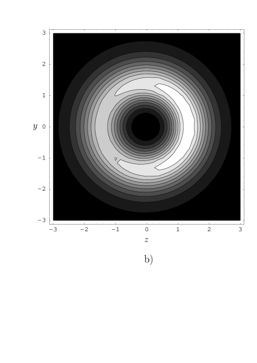
FIG. 5.: Baryon charge distribution $B_{0}$ of the skyrmion embedded in ${}^{12}C$ in the $yz$ plane (a) and its projection (equal baryon charge distribution areas) onto this plane (b), where $y$, $z$ are dimensionless variables. The distance from the center of the nucleus $R$ is equal to $1.266$ fm. This corresponds to maximum value of the leading deformation parameter $\gamma_{1}$. The center of the nucleus is situated on the negative side of the axis $z$. The strength of the baryon charge distribution corresponding to the different area is represented by light/dark shading. The baryon density is lower if the area is darker. The values of the deformation parameters at this place are $\delta r_{S}=-0.0476$ fm, $\gamma_{1}=-0.0763$, $\gamma_{2}=0.028$, $\gamma_{3}=-0.0039$, $\delta_{1}=0.0029$ and $\delta_{2}=-0.0003$.

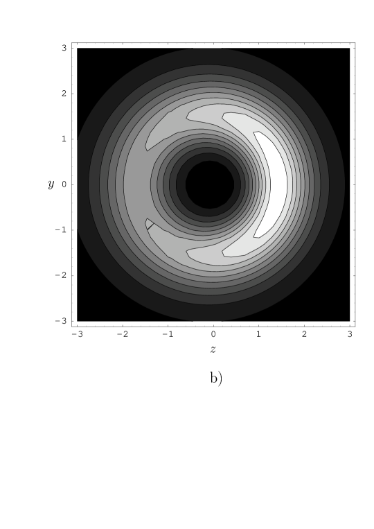
FIG. 6.: As in the Fig. 5 but for the skyrmion embedded in ${}^{56}Fe$, where $R=4.275$ fm. The values of the deformation parameters at this place are $\delta r_{S}=-0.1464$ fm, $\gamma_{1}=-0.1610$, $\gamma_{2}=0.0326$, $\gamma_{3}=0.0108$, $\delta_{1}=0.0026$ and $\delta_{2}=-0.0002$.

FIG. 7.: Mass dependence of a nucleon embedded in various nuclei as a function of the fraction $R/R_{A}$, where $R$ is the distance between the centers of nucleus and nucleon and $R_{A}$ is the radius of the nucleus (see eq. (49)). The solid line represents this dependence for the nucleon in ¹⁶O, while the dashed and dotted lines represent this dependence for ⁵⁶Fe and ¹⁹⁸Au, respectively.

FIG. 8.: The $R/R_{A}$ dependence of isoscalar (top figure) and isovector (bottom figure) intrinsic quadrupole moments of a nucleon embedded in various nuclei. For the notations see Fig. 7.

REFERENCES

- [1] A.M. Rakhimov, M.M. Musakhanov, F.C. Khanna and U.T. Yakhshiev, Phys. Rev. C58, 1738 (1998).
-
[2]
A.M. Rakhimov, F.C. Khanna, U.T. Yakhshiev, M.M. Musakhanov,
Nucl. Phys. A643, 383 (1998);
M. Musakhanov, A. Rakhimov, U. Yakhshiev, Z. Kanokov, Phys. Atom. Nucl. (Russ. J. Nucl. Phys.) 62, 1988 (1999). - [3] Ulf-G. Meißner, Phys. Rev. Lett. 62, 1013 (1989); Phys. Lett. B220, (1989); Nucl. Phys. A503, 801 (1989).
-
[4]
I. Klebanov, Nucl. Phys. B262, 133 (1985);
N.K. Glendenning, Phys. Rev. C34, 1072 (1986);
E. Wüst, G.E. Brown and A.D. Jackson, Nucl. Phys. A 468, 450 (1987);
A.S. Goldhaber and N.S. Manton, Phys. Lett. B198, 231 (1987);
T.S. Walhout, Nucl. Phys. A484, 397 (1988); Nucl. Phys. A 519, 816 (1990);
A.D. Jackson, A. Wirzba and L.S. Castillejo, Phys. Lett. B198, 315 (1987); Nucl. Phys. A486, 634 (1988);
M. Kugler and S. Shtrikman, Phys. Lett. B208, 491 (1988); Phys. Rev. D40, 3421 (1989);
L.S. Castillejo et al., Nucl. Phys. A501, 801 (1989);
H. Forkel et al., Nucl. Phys. A504, 818 (1989);
A.D. Jackson, C. Weiss and A. Wirzba, Nucl. Phys. A529, 741 (1991);
A. Wirzba, in “Baryons as Skyrme Solitons”, G. Holzwarth (ed.), World Scientific, Singapore, 1993;
W.K. Baskerville, Nucl. Phys. A596, 611 (1996);
P. Amore, Nuovo Cim. A111, 493 (1998). - [5] V. Vento, G. Baym and A.D. Jackson, Phys. Lett. B102, 97 (1981).
- [6] U.B. Kaulfuß and Ulf-G. Meißner, Phys. Rev. D31, 3024 (1985).
- [7] A. Rakhimov, T. Okazaki, M.M. Musakhanov, F.C. Khanna, Phys. Lett. B378, 12 (1996).
-
[8]
C. Hajduk, B. Schwesinger,
Phys. Lett. B140, 172 (1984);
C. Hajduk, B. Schwesinger, Nucl. Phys. A453, 620 (1986). -
[9]
V.B. Kopeliovich, B.E. Stern,
Sov. J. JETP Lett. 45, 165 (1987);
V.B. Kopeliovich, Sov. J. Nucl.Phys. 47, 1495 (1988);
B.E. Stern, Sov. J. Nucl.Phys. 49, 530 (1989);
V.B. Kopeliovich, Russ. J. Nucl.Phys. 56, 160 (1993). -
[10]
V.A. Nikolaev,
Sov. J. Part. Nucl. 20, 401 (1989);
V.A. Nikolaev, O.G. Tkachev, Sov. J. Part. Nucl. 21, 1499 (1990);
R.M. Nikolaeva, V.A. Nikolaev, O.G. Tkachev, Sov. J. Part. Nucl. 23, 542 (1992). - [11] T. Kurihara, H. Kanada, T. Otofuji, S. Saito, Prog. Theor. Phys. 81, 858 (1989).
- [12] E.B. Bogomolniy, V.A. Fateev, Sov. J. Nucl. Phys. 37, 228 (1983).
- [13] U.T. Yakhshiev, N.A.Taylanov, Uzb. J. Phys. 2, 114 (2000).
-
[14]
E. Braaten and L. Carson, Phys. Rev. Lett. 56,
1897 (1986);
E. Braaten and L. Carson, Phys. Rev. D38, 3525 (1988);
E. Braaten, S. Townsend and L. Carson, Phys. Lett. B235, 147 (1990);
N.S. Manton, Phys. Lett. B192, 177 (1987);
M.F. Atiyah and N.S. Manton, Commun. Math. Phys. 153, 391 (1993);
R.A. Leese and N.S. Manton, Nucl. Phys. A572, 575 (1994);
C.J. Houghton, N.S. Manton and P.M. Sutcliffe, Nucl. Phys. B510, 507 (1998). -
[15]
I. Zahed et al., Phys. Rev. D31, 1114 (1985);
C.-K. Lin, Nucl. Phys. A449, 673 (1986);
J. Wambach, H.W. Wyld and H.M. Sommermann, Phys. Lett. B186, 272 (1987);
T. Otofuji et al., Prog. Theor. Phys. 78, 527 (1987);
I. Mishustin, Sov. Phys. JETP 71, 21 (1990);
F. Leblond and L. Marleau, Phys. Rev. D58, 054002 (1998). - [16] A. Wirzba and V. Thorsson, Nucl. Phys. A589, 633 (1985).
- [17] T. Ericson and W. Weise, Pions and Nuclei (Claredon, Oxford, 1988).
- [18] A. Akhiezer, A.G. Sitenko, V.K. Tartakovski, Nuclear electrodynamics (Springer Verlag, 1994).
-
[19]
G.S. Adkins, C.R. Nappi and E. Witten,
Nucl. Phys. B228, 552 (1983);
G.S. Adkins and C.R. Nappi, ibid. B233, 109 (1984). - [20] J. Schechter, Phys Rev. D21, 3393 (1980); H. Gomm et al., Phys. Rev. D33, 3476 (1986).
- [21] Ulf-G. Meissner, A. Rakhimov and U.T. Yakhshiev, Phys. Lett. B473, 200 (2000).
- [22] Ulf-G. Meißner, Phys. Rep. 161, 213 (1988).
- [23] J.V. Noble, Phys. Rev. Lett. 46, 412 (1981).
- [24] I. Sick, Phys. Lett. B157, 13 (1985).
- [25] A. Bohr and B.R. Mottelson, Nuclear Structure, Vol. II, Nuclear Deformations (W.A. Benjamin, Reading, Massachusetts, 1975).