Low lying $S=-1$ excited baryons and chiral symmetry

Abstract

The s-wave meson-baryon interaction in the $S=-1$ sector is studied by means of coupled-channels, using the lowest-order chiral Lagrangian and the N/D method to implement unitarity. The loops are regularized using dimensional renormalization. In addition to the previously studied $\Lambda(1405)$, employing this chiral approach leads to the dynamical generation of two more s-wave hyperon resonances, the $\Lambda(1670)$ and $\Sigma(1620)$ states. We make comparisons with experimental data and look for poles in the complex plane obtaining the couplings of the resonances to the different final states. This allows us to identify the $\Lambda(1405)$ and the $\Lambda(1670)$ resonances with $\bar{K}N$ and $K\Xi$ quasibound states, respectively.

1 Introduction

The low-energy $K^{-}N$ scattering and transition to coupled channels is one of the cases of successful application of chiral dynamics in the baryon sector. The studies of [1] and [2] showed that one could obtain an excellent description of the low-energy data starting from chiral Lagrangians and using the multichannel Lippman-Schwinger equation to account for multiple scattering and unitarity in coupled channels. By including all open channels above threshold and fitting a few chiral parameters of the second-order Lagrangian one could obtain a good agreement with the data at low energies. This line of work was continued in [3], where all coupled channels were included that could be arranged from the octet of pseudoscalar Goldstone bosons and the baryon ground state octet. In Ref.[3] it was demonstrated that using the Bethe-Salpeter equation (BSE) with coupled channels and using the lowest-order chiral Lagrangians, together with one cut off to regularize the intermediate meson-baryon loops, a good description of all low-energy data was obtained. One of the novel features with respect to other approaches using the BSE is that the lowest-order meson-baryon amplitudes, playing the role of a potential, could be factorized on shell in the BSE, and thus the set of coupled-channels integral equations became a simple set of algebraic equations, thus technically simplifying the problem. The justification of this procedure is seen in a more general way in the treatment of meson-meson interactions using chiral Lagrangians and the N/D method in [4]. One uses dispersion relations and shows that neglecting the effects of the left-hand singularity (also shown to be small there) one needs only the on-shell scattering matrix from the lowest-order Lagrangian, and the eventual effects of higher-order Lagrangians are accounted for in terms of subtractions in the dispersion integrals. The N/D method has also been recently applied to study pion-nucleon dynamics in Ref. [5].

The work of Ref.[3] was reanalyzed recently [6] from the point of view of the N/D method and dispersion relations, leading formally to the same algebraic equations found in [3]. There are also technical novelties in the regularization of the loop function, which is done using dimensional regularization in Ref.[6], while it was regularized with a cut off in Ref.[3].

One of the common findings shared by all the theoretical approaches is the dynamical generation of the $\Lambda(1405)$ resonance which appears with the right width, and at the correct position, with the choice of a cut off of natural size. This natural generation from the interaction of the meson-baryon system with the lowest-order Lagrangian allows us to identify that state as a quasibound meson-baryon state. This would explain why ordinary quark models have had so many problems explaining this resonance [7].

In ordinary quark models the $\Lambda(1405)$ resonance would mostly be a SU(3) singlet of $J^{P}=1/2^{-}$ and there would be an associated octet of s-wave excited $J^{P}=1/2^{-}$ baryons that would include the N*(1535), the $\Lambda(1670)$, the $\Sigma(1620)$ and a $\Xi^{*}$ state. In the chiral approach one would also expect the appearance of such a nonet of resonances. In fact, it appears naturally in the approach of Ref.[3], with a degenerate octet, when setting all the masses of the octet of stable baryons equal on one side and the masses of the octet of pseudoscalar mesons equal on the other side. Yet, to obtain this result it is essential that the coupled channels do not omit any of the channels that can be constructed from the octet of pseudoscalar mesons and the octet of stable baryons.

The lowest-order Lagrangian involving the octet of pseudoscalar mesons and the $1/2^{+}$ baryons is given in [8, 9, 10, 11]. At lowest order in momentum, that we will keep in our study, the interaction Lagrangian reads

$$L_{1}^{(B)}=<\bar{B}i\gamma^{\mu}\frac{1}{4f^{2}}[(\Phi\partial_{\mu}\Phi-\partial_{\mu}\Phi\Phi)B-B(\Phi\partial_{\mu}\Phi-\partial_{\mu}\Phi\Phi)]>\ ,$$ (1)

where $\Phi$ and $B$ are the SU(3) matrices for the mesons and baryons, respectively and the symbol $<>$ stands for the trace of the resulting SU(3) matrix. The Lagrangian of Eq. (1) leads to a common structure of the type $\bar{u}\gamma^{u}(k_{\mu}+k^{\prime}_{\mu})u$ for the different channels, where $u,\bar{u}$ are the Dirac spinors and $k,k^{\prime}$ the momenta of the incoming and outgoing mesons.

We take the $K^{-}p$ state and all those that couple to it within the chiral scheme, namely $\bar{K}^{0}n$, $\pi^{0}\Lambda$, $\pi^{0}\Sigma^{0}$, $\pi^{+}\Sigma^{-}$, $\pi^{-}\Sigma^{+}$, $\eta\Lambda$, $\eta\Sigma^{0}$, $K^{0}\Xi^{0}$ and $K^{+}\Xi^{-}$. Hence we have a problem with ten coupled channels.

The lowest-order amplitudes for these channels are easily evaluated from Eq. (1) and are given by

$$V_{ij}=-C_{ij}\frac{1}{4f^{2}}\bar{u}(p_{i})\gamma^{\mu}u(p_{j})(k_{j\mu}+k_{i\mu})$$ (2)

where $p_{j},p_{i}(k_{j},k_{i})$ are the initial, final momenta of the baryons (mesons). For low energies one can write this amplitude as

$$V_{ij}=-C_{ij}\frac{1}{4f^{2}}(2\sqrt{s}-M_{Bi}-M_{Bj})\left(\frac{M_{Bi}+E}{2M_{Bi}}\right)^{1/2}\left(\frac{M_{Bj}+E^{\prime}}{2M_{Bj}}\right)^{1/2}\,,$$ (3)

and the matrix $C_{ij}$, which is symmetric, is given in [3].

Note that the use of physical masses in Eq. (3) is introducing effectively some contributions of higher orders in the chiral counting. In the standard chiral approach one would be using the average mass of the octets in the chiral limit and higher order Lagrangians involving SU(3) breaking terms would generate the mass differences. By introducing the physical masses one guarantees that the phase space for the reactions, thresholds and unitarity in coupled channels are respected from the beginning. We also use in our approach an average value for the pseudoscalar meson decay constant, $f=1.15f_{\pi}$, as done in [3].

We shall construct the amplitudes using the isospin formalism for which we must use average masses for the $K$ $(K^{0},K^{+})$, $\bar{K}$ $(K^{-},\bar{K}^{0}$), $N$ $(p,n)$, $\pi$ ($\pi^{+},\pi^{0},\pi^{-}$), $\Sigma$ ($\Sigma^{+},\Sigma^{0},\Sigma^{-}$) and $\Xi$ $(\Xi^{-},\Xi^{0})$ states. The isospin states are given in [3].

We have four $I=0$ channels, $\bar{K}N,\pi\Sigma$, $\eta\Lambda$ and $K\Xi$, while there are five $I=1$ channels, $\bar{K}N,\pi\Sigma,\pi\Lambda,\eta\Sigma$ and $K\Xi$. The transition matrix elements in isospin formalism read like Eq. (3) substituting the $C_{ij}$ coefficients by $D_{ij}$ for $I=0$ and by $F_{ij}$ for $I=1$, with the $D_{ij}$ and $F_{ij}$ coefficients given in [3].

In [6], using the N/D method of [4] for this particular case it was proved that the scattering amplitude could be written by means of the algebraic matrix equation

$$T=[1-V\,G]^{-1}\,V$$ (4)

with $V$ the matrix of Eq. (3) evaluated on shell, or equivalently

$$T=V+V\,G\,T$$ (5)

with $G$ a diagonal matrix given by

$$G_{l} = i\,\int\frac{d^{4}q}{(2\pi)^{4}}\,\frac{M_{l}}{E_{l}(\vec{q}\,)}\,\frac{1}{k^{0}+p^{0}-q^{0}-E_{l}(\vec{q}\,)+i\epsilon}\,\frac{1}{q^{2}-m^{2}_{l}+i\epsilon}$$ (6)

$$= \int^{q_{\rm max}}\,\frac{d^{3}q}{(2\pi)^{3}}\,\frac{1}{2\omega_{l}(\vec{q}\,)}\,\frac{M_{l}}{E_{l}(\vec{q}\,)}\,\frac{1}{p^{0}+k^{0}-\omega_{l}(\vec{q}\,)-E_{l}(\vec{q}\,)+i\epsilon}$$

which depends on $p^{0}+k^{0}=\sqrt{s}$ and $q_{\rm max}$.

One can see that Eq. (5) is just the Bethe Salpeter equation but with the $V$ matrix factorized on shell, which allows one to extract the scattering matrix $T$ trivially, as seen in Eq. (4).

The analytical expression for $G_{l}$ can be obtained from [12] using a cut off and from [6] using dimensional regularization,

$$G_{l} = i2M_{l}\int\frac{d^{4}q}{(2\pi)^{4}}\,\frac{1}{(P-q)^{2}-M_{l}^{2}+i\epsilon}\,\frac{1}{q^{2}-m^{2}_{l}+i\epsilon}$$ (7)

$$= \frac{2M_{l}}{16\pi^{2}}\left\{a_{l}(\mu)+\ln\frac{M_{l}^{2}}{\mu^{2}}+\frac{m_{l}^{2}-M_{l}^{2}+s}{2s}\ln\frac{m_{l}^{2}}{M_{l}^{2}}+\right.$$

$$\phantom{\frac{2M}{16\pi^{2}}}+\frac{\bar{q}_{l}}{\sqrt{s}}\left[\ln(s-(M_{l}^{2}-m_{l}^{2})+2\bar{q}_{l}\sqrt{s})+\ln(s+(M_{l}^{2}-m_{l}^{2})+2\bar{q}_{l}\sqrt{s})\right.$$

$$\left.\phantom{\frac{2M}{16\pi^{2}}+\frac{\bar{q}_{l}}{\sqrt{s}}}\left.-\ln(-s+(M_{l}^{2}-m_{l}^{2})+2\bar{q}_{l}\sqrt{s})-\ln(-s-(M_{l}^{2}-m_{l}^{2})+2\bar{q}_{l}\sqrt{s})\right]\right\}\ ,$$

which has been rewritten in a convenient way to show how the imaginary part of $G_{l}$ is generated and how one can go to the unphysical Riemann sheets in order to identify the poles. The dimensional regularization scheme is preferable if one goes to higher energies where the on-shell momentum of the intermediate states is not reasonably smaller than the cut off.

The coupled set of Eqs. (4) were solved in [3] using a cut off momentum of 630 MeV in all channels. Changes in the cut off can be accommodated in terms of changes in $\mu$, the regularization scale in the dimensional regularization formula for $G_{l}$, or in the subtraction constant $a_{l}$. In order to obtain the same results as in [3] at low energies, we set $\mu$ equal to the cut off momentum of 630 MeV (in all channels) and then find the values of the subtraction constants $a_{l}$ such as to have $G_{l}$ with the same value with the dimensional regularization formula (Eq. (7)) and the cut off formula (Eq. (6)) at the $\bar{K}N$ threshold. This determines the values

$$\begin{array}[]{lll}a_{{\bar{K}}N}=-1.84{}{}&a_{\pi\Sigma}=-2.00{}{}&a_{\pi\Lambda}\,=-1.83\\ a_{\eta\Lambda}\,\,=-2.25{}{}&a_{\eta\Sigma}=-2.38{}{}&a_{K\Xi}=-2.52\ .\end{array}$$ (8)

In this way we guarantee that we obtain the same results at low energies as in [3] and we find indeed that this is the case when we repeat the calculation with the new $G_{l}$ of Eq. (7). Then we extend the results at higher energies, looking for the eventual appearance of new resonances.

The solid lines of Figs. 1 and 2 show the results for the real and imaginary parts of the $I=0$ amplitudes for $\bar{K}N\to\bar{K}N$ and $\bar{K}N\to\pi\Sigma$, respectively. Both channels clearly display the signal from the $\Lambda(1670)$ resonance, although large background contributions are present in the amplitudes as well.

Figure 1: $\bar{K}N\to\bar{K}N$ amplitude in the $I=0$ channel. Data are taken from Ref. [13].

Figure 2: $\bar{K}N\to\pi\Sigma$ amplitude in the $I=0$ channel. Data are taken from Ref. [13].

The normalization of the amplitudes shown in Figs. 1 and 2 is different from the one of Eq. (4). We shall call $T_{M}$ the plotted amplitudes and the relationship to our former amplitudes is given by

$$T_{M,ij}=-T_{ij}\frac{\sqrt{M_{i}M_{j}p_{i}p_{j}}}{4\pi\sqrt{s}}$$ (9)

The normalization of $T_{M}$ is particularly suited to analyze the data in terms of the speed plot [14]. One has the amplitude written as

$$T_{M,ij}(W)=T^{BG}_{M,ij}(W)-\frac{x\,\,\Gamma/2\,\,{\rm e}^{i\phi}}{W-M_{R}+i\Gamma/2}$$ (10)

with $x=\sqrt{\Gamma_{i}\Gamma_{j}}/\Gamma$, where $\Gamma$, $\Gamma_{i}$, $\Gamma_{j}$ are, respectively, the total width and the partial decay widths of the resonance into the $i,j$ channels.

The speed is defined as

$$Sp_{ij}(W)=\left|\frac{dT_{M,ij}}{dW}\right|\simeq\frac{x\Gamma/2}{(W-M_{R})^{2}+\Gamma^{2}/4}\ ,$$ (11)

where the second equality assumes that the background is smoothly dependent on the energy and does not contribute significantly to the derivative.

In Fig. 3 we show the obtained speed $Sp_{ij}(W)$ for different transitions, $\bar{K}N\to\bar{K}N$ (solid line), $\bar{K}N\to\eta\Lambda$ (dotted line) and $\bar{K}N\to\pi\Sigma$ (dashed line). As is evident from the plots in Fig. 3, the background induced by the already opened meson-baryon channels in the region of interest is quite smooth, since an approximate Breit-Wigner shape is obtained from the derivative of the amplitudes. On the other hand, the resonance region we study does indeed lie above the two-pion threshold for both $\Lambda$ and $\Sigma$ production. Such threshold openings could show up in some form as a non-smooth background contribution. However, there is no empirical evidence that any of the s-channel hyperon resonances under investigation here couple strongly to the two-pion channel, hence, we do not expect the Breit-Wigner shape of Fig. 3 to be modified by the inclusion of extra inelastic channels.

The study of the speed plots shown in Fig. 3 allows us to obtain the energy $M_{R}=1708$ MeV, the total width $\Gamma=40$ MeV, and the branching ratios, $B_{\bar{K}N}=48$%, $B_{\eta\Lambda}=45$%, and $B_{\pi\Sigma}=7$%. Experimentally, one has $M_{R}=1660-1680$ MeV, $\Gamma=25-50$ MeV, $B_{\bar{K}N}=15-25$%, $B_{\eta\Lambda}=15-35$%, and $B_{\pi\Sigma}=15-35$% [15]. We seem to overestimate the $\bar{K}N$ and $\eta\Lambda$ branching ratios and underestimate the $\pi\Sigma$ one.

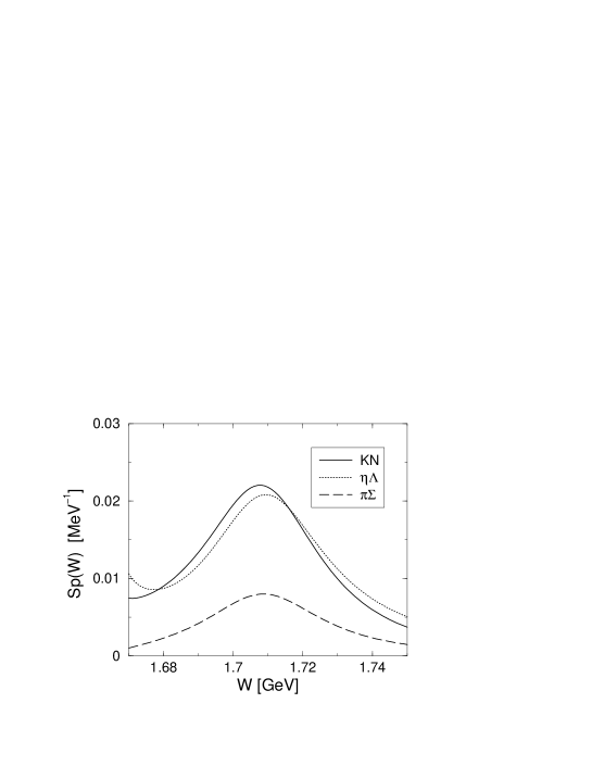
Figure 3: Speed plot for the amplitudes $\bar{K}N\to\bar{K}N$ (solid line), $\bar{K}N\to\eta\Lambda$ (dotted line) and $\bar{K}N\to\pi\Sigma$ (dashed line).

Comparison of our results with the experimental data in Figs. 1 and 2 shows qualitative but not quantitative agreement. This is not surprising since no parameters have been fitted to these data, but rather we have chosen the low-energy parametrization of our theory which contained only one free parameter, the cut off to regularize the loops. We now exploit the freedom that the theory has by changing the parameters $a_{l}$. However, this must be accomplished in a way that does not ruin the very good agreement with the low-energy data, found in Ref.[3]. We find that the results at low energies are very insensitive to changes in the $a_{K\Xi}$ parameter, but they are sensitive to changes in $a_{{\bar{K}}N}$, $a_{\pi\Sigma}$ and $a_{\eta\Lambda}$. On the other hand, the position of the $\Lambda(1670)$ resonance is quite sensitive to changes in the $a_{K\Xi}$ parameter and only moderately sensitive to $a_{\bar{K}N}$, $a_{\pi\Sigma}$ and $a_{\eta\Lambda}$. This allows us to fine tune the parameter $a_{K\Xi}$ (without changing the other $a_{l}$ parameters) in order to better reproduce the position of the resonance found by experiment while maintaining the agreement found at low energies. Figs. 1 and 2 also display the results using $a_{K\Xi}=-2.67$ (dashed lines). We see that a change of 6% in this parameter moves the position of the resonance by $28$ MeV and it agrees better with experiment. The values of the resonance mass, width and branching ratios obtained now are $M_{R}=1679$ MeV, the total width $\Gamma=40$ MeV, and the branching ratios $B_{\bar{K}N}=61$%, $B_{\eta\Lambda}=30$%, and $B_{\pi\Sigma}=9$%.

Comparison of the theoretical results for ${\bar{K}}N\to{\bar{K}}N$ with the data shows agreement for the imaginary part within errors, while our prediction for the real part below the resonance differs from the data by what appears to be a large constant background term. This discrepancy needs to be looked at with some perspective. The contribution of the real part to the cross section from the experimental data is negligible and is only 10 percent in the theoretical case. On the other hand, our results around $\sqrt{s}=1440$ MeV, the $\bar{K}N$ threshold, are in good agreement with the data for the $K^{-}p$ and $K^{-}n$ scattering lengths, which would suggest some discrepancy at low energies between the data shown in Fig. 1 [13] and those of [16] and [17].

In Fig. 2 we display the $I=0$ $\bar{K}N\to\pi\Sigma$ amplitude. The theoretical amplitude shows the resonance features with the same pattern as the experiment, both for the real as for the imaginary parts. Yet there is disagreement with the data in the imaginary part, again with an apparent background missing for the theoretical prediction. Once again, the discrepancy looks puzzling since up to $\sqrt{s}=1460$ MeV, and even beyond where the s-wave is still dominant, the agreement of the present model with the experimental cross sections for $K^{-}p\to\pi^{-}\Sigma^{+},\pi^{+}\Sigma^{-},\pi^{0}\Sigma^{0}$ is very good [3].

We should note that the errors plotted in Figs. 1 and 2 correspond to the reasonable guesses of Ref. [18], but there are actual deviations between the data of [13], [19] and [20]. Due to the large background in the experimental analysis, the interference effects with the resonance are more apparent, leading to a larger branching ratio to the $\pi\Sigma$ channel than the theory predicts.

We can also compare the results of the model with the recent data on the $K^{-}p\to\eta\Lambda$ reaction [21], which improve on the older experiments [22]. The shape of the results and the position of the peak that we obtain agree well with the data for a parameter $a_{K\Xi}=-2.67$ but we get a strength at the peak of $\sigma=2.7$ mb, about a factor of two larger than the latest experimental value of $\sigma=1.4$ mb. This reflects the fact that our predicted $\bar{K}N$ branching ratio overestimates the experimental value.

We have studied the reactions $K^{-}p\to K^{+}\Xi^{-}$ and $K^{-}p\to K^{0}\Xi^{0}$, which take place at energies beyond $\sqrt{s}=1.815$ GeV, hence above the position of the $\Lambda(1670)$ resonance. Around a laboratory $K^{-}$ momentum of $1.6$ GeV/c, and using $a_{K\Xi}=-2.67$, our model predicts a cross section of $0.17$ mb for the reaction $K^{-}p\to K^{+}\Xi^{-}$, which compares favourably with the experimental value of $0.16-0.18$ mb [23, 24]. For the reaction $K^{-}p\to K^{0}\Xi^{0}$ we find a cross section of $0.24$ mb at $1.6$ GeV/c, which overestimates by almost a factor of three the experimental value of $0.08-0.1$ mb [24].

In the $I=1$ channel we find only rough agreement with the data in the $\bar{K}N\to\bar{K}N$ and $\bar{K}N\to\pi\Sigma$ amplitudes, but, just like the data, we find no evidence of a resonance signal that would allow us to identify the $\Sigma(1620)$ resonance. Clearly, the absence of a signal even in some of the experimental amplitudes has lead to classifying the $\Sigma(1620)$ as only a 2-star resonance. However, the absence of such a resonance would be somewhat surprising since we expect to get an octet of meson-baryon resonances and so far only a singlet and the $I=0$ part of the octet (eventually mixed between themselves) have appeared. Since we do not see this state in the amplitudes at real energies we look for a pole in the complex plane. We go directly to the second Riemann sheet, which we take in our case as the one where the momenta of the channels which are open at energy $W$, with ${\rm Re}(z)=W$, are taken negative in $G_{l}$.

Near the poles the amplitudes that we are analyzing behave as

$$T_{ij}\simeq\frac{g_{i}g_{j}}{z-z_{R}}~{}~{}~{}~{};~{}~{}~{}~{}T_{M,ij}\simeq\frac{x\Gamma/2{\rm e}^{i\phi^{\prime}}}{z-z_{R}}\ .$$ (12)

Thus, the residues of the $T_{ij}$ matrix give the product of the coupling of the resonance to the $i,j$ channels, while the residues of the $T_{M,ij}$ give one half of the product of the two partial decay widths. The first one of equations (12) determines the coupling of the resonance to different final states, which are well defined even if these states are closed in the decay of the resonance.

The search of the poles leads us, using $a_{K\Xi}=-2.52$, to the values $M_{R}=1708+i21$ MeV, $\Gamma=42$ MeV, $B_{\bar{K}N}=47$%, $B_{\eta\Lambda}=47$%, and $B_{\pi\Sigma}=6$%, in remarkable agreement with the values obtained from the speed plot. For $a_{K\Xi}=-2.67$, we obtain $M_{R}=1680+i20$ MeV, $\Gamma=40$ MeV, $B_{\bar{K}N}=54$%, $B_{\eta\Lambda}=38$%, and $B_{\pi\Sigma}=8$%.

The couplings obtained for the $\Lambda(1670)$ resonance, using $a_{K\Xi}=-2.52$, are

$$\mid g_{{\bar{K}}N}\mid^{2}=0.51~{}~{}~{}~{}\mid g_{\pi\Sigma}\mid^{2}=0.052~{}~{}~{}~{}\mid g_{\eta\Lambda}\mid^{2}=1.0~{}~{}~{}~{}\mid g_{K\Xi}\mid^{2}=11\ ,$$ (13)

and, using $a_{K\Xi}=-2.67$, we obtain

$$\mid g_{{\bar{K}}N}\mid^{2}=0.61~{}~{}~{}~{}\mid g_{\pi\Sigma}\mid^{2}=0.073~{}~{}~{}~{}\mid g_{\eta\Lambda}\mid^{2}=1.1~{}~{}~{}~{}\mid g_{K\Xi}\mid^{2}=12\ .$$ (14)

It is also interesting to display the results of the complex plane search for the $\Lambda(1405)$ resonance. We find

$$M_{R}=(1426+i16)~{}{\rm MeV}~{}~{}(\Gamma=32~{}{\rm MeV})$$

$$\mid g_{{\bar{K}}N}\mid^{2}=7.4~{}~{}~{}~{}\mid g_{\pi\Sigma}\mid^{2}=2.3~{}~{}~{}~{}\mid g_{\eta\Lambda}\mid^{2}=2.0~{}~{}~{}~{}\mid g_{K\Xi}\mid^{2}=0.12\ ,$$

with only the $\pi\Sigma$ channel open for the decay.

We have also performed a search in the $I=1$ channel and we indeed find a pole at

$$M_{R}=(1579+i264)~{}{\rm MeV}~{}~{}(\Gamma\sim 528~{}{\rm MeV})\ ,$$

from the model with $a_{K\Xi}=-2.67$. The couplings obtained are

$$\mid g_{{\bar{K}}N}\mid^{2}=2.6~{}~{}~{}~{}\mid g_{\pi\Sigma}\mid^{2}=7.2~{}~{}~{}~{}\mid g_{\pi\Lambda}\mid^{2}=4.2~{}~{}~{}~{}\mid g_{\eta\Sigma}\mid^{2}=3.5~{}~{}~{}~{}\mid g_{K\Xi}\mid^{2}=12\ .$$

We find that the agreement with the PDG [15] is quite good for the case of the $\Lambda(1405)$. For the case of the $\Lambda(1670)$ we find a good agreement with the total width, but the partial decay widths to the $\bar{K}N$ and $\eta\Lambda$ channels is somewhat overpredicted while the partial decay width to the $\pi\Sigma$ channel that we obtain is a bit too small. For the case of the $\Sigma(1620)$ resonance we find a very large width which may be the reason why this state does not provide a clearer signal in the scattering amplitudes.

The analysis of the couplings is very interesting. In the case of the $\Lambda(1405)$ state the coupling to the $\bar{K}N$ channel is found to be very large, while the coupling to the other channels is very small. This would allow us to identify this resonance as a quasibound $\bar{K}N$ state in the present approach. Similarly, we find that the $\Lambda(1670)$ resonance has a large coupling to the $K\Xi$ channel and unusually small couplings to the other final states. This is responsible for the small width of the resonance in spite of the large phase space open for decay into the different channels. The large coupling to the $K\Xi$ channel allows identifying this state as a $K\Xi$ quasibound state in the present approach. By contrast, the $\Sigma(1620)$ resonance has couplings of normal size to all channels, and, given the large phase space available, it has a sizable decay width into any of the channels and hence a considerably larger total width.

In summary, we have demonstrated that the chiral approach to the $\bar{K}N$ and the other coupled channels, which proved so successful at low energies, extrapolates smoothly to higher energies and provides the basic features of the scattering amplitudes, generating the resonances which would complete the states of the nonet of the $J^{P}=1/2^{-}$ excited states. The qualitative description of the data without adjusting any parameters is telling us that the basic information on the dynamics of these processes is contained in the chiral Lagrangians. There is still some freedom left with the chiral symmetry breaking terms. In our formulation they would go into the $a_{l}$ subtraction constants, and the use of different decay constants for each meson, by means of which one could obtain a better description of the data. However, before proceeding in this direction, and eventually introduce further chiral symmetry breaking terms, it would be important to sort out the apparent discrepancies between different sets of data. The analysis of the poles and the couplings of the resonances to the different channels lead us to identify the strong coupling of the $\Lambda(1405)$ resonance to the $\bar{K}N$ state and the large coupling of the $\Lambda(1670)$ resonance to the $K\Xi$ state, allowing us to classify these resonances as quasibound states of $\bar{K}N$ and $K\Xi$, respectively.

Acknowledgments

E. O. and C. B. wish to acknowledge the hospitality of the University of Barcelona and A. R. and C. B. that of the University of Valencia, where part of this work was done. We would also like to acknowledge some useful discussions with J.A. Oller and U.G. Meissner. This work is also partly supported by DGICYT contract numbers BFM2000-1326, PB98-1247, by the EU TMR network Eurodaphne, contract no. ERBFMRX-CT98-0169, and by the US-DOE grant DE-FG02-95ER-40907.

References

- [1] N. Kaiser, P. B. Siegel and W. Weise, Nucl. Phys. A594 (1995) 325
- [2] N. Kaiser, T. Waas and W. Weise, Nucl. Phys. A612 (1997) 297
- [3] E. Oset and A. Ramos, Nucl. Phys. A635 (1998) 99
- [4] J.A. Oller and E. Oset, Phys. Rev. D60 (1999) 074023
- [5] J.A. Oller and U.G. Meissner, Nucl. Phys. A673 (2000) 311
- [6] J.A. Oller and U.G. Meissner, Phys. Lett. B500 (2001) 263
- [7] N. Isgur and G. Karl, Phys. Rev. D18 (1978) 4187; ibid. D20 (1979) 1191; S. Capstick and W. Roberts, Phys. Rev. D49 (1994) 4570
- [8] A. Pich, Rep. Prog. Phys. 58 (1995) 563
- [9] G. Ecker, Prog. Part. Nucl. Phys. 35 (1995) 1
- [10] V. Bernard, N. Kaiser and U. G. Meissner, Int. J. Mod. Phys. E4 (1995) 193
- [11] U. G. Meissner, Rep. Prog. Phys. 56 (1993) 903
- [12] J. A. Oller, E. Oset and J. R. Peláez, Phys. Rev. D59 (1999) 074001
- [13] G. P. Gopal et al. Nucl. Phys. B119 (1977) 362
- [14] G. Hoehler, -Newsletter 9 (1993) 1
- [15] D. E. Groom et al., The European Physical Journal C15 (2000) 1
- [16] A. D. Martin, Nucl. Phys. B179 (1981)33
- [17] M. Iwasaki et al. , Phys. Rev. Lett. 78 (1997) 3067
- [18] M. Th. Keil, G. Penner and U. Mosel, Phys. Rev. C63 (2001) 045202
- [19] W. Langbein and F. Wagner, Nucl. Phys. B47 (1972) 477
- [20] M. Alston-Garnjost et al., Phys. Rev. D18 (1978) 182
- [21] B. Nefkens, in Proceedings of the Workshop on The Physics of Excited Nucleons, NSTAR2001, Eds. D. Drechsel and L. Tiator (World Scientific, 2001) 427; D.M. Manley, in Proceedings of the 9th International Symposium on Meson-Nucleon Physics and the Structure of the Nucleon, N Newsletter 16 (2001) 68.
- [22] G. W. London et al., Nuc. Phys. B85 (1975) 289; D. F. Baxter et al., Nuc. Phys. B67 (1973) 125; R. Rader et al., Nuovo Cim. 16A (1973) 178; D. Berley et al., Phys. Rev. Lett. 15 (1965) 641
- [23] J. Griselin et al. Nuc. Phys. B93 (1975) 189
- [24] A. de Bellefon et al., Nuovo Cim. 7A (1972) 567