Statistical models of nuclear level densities.

Abstract

We present calculations of nuclear level densities that are based upon the detailed microphysics of the interacting shell model yet are also computationally tractable. To do this, we combine in a novel fashion several previously disparate ideas from statistical spectroscopy, namely partitioning of the model space into subspaces, analytic calculations of moments up to fourth order directly from the two-body interaction, and Zuker’s binomial distribution. We get excellent agreement with full scale interacting shell model calculations. We also calculate “ab initio” the level densities for ²⁹Si and ⁵⁷Co and get reasonable agreement with experiment.

Reliable nuclear level densities are important for the theoretical estimates of nuclear reaction rates in nucleosynthesis [1]. The neutron-capture cross sections are approximately proportional to the corresponding level densities around the nuclear resonance region. The competition between neutron-capture and $\beta$ decay determines the fate of the s and r processes. Level densities can be extracted experimentally [2], but reaction network calculations require cross-sections for hundreds or thousands of nuclides, many of them short-lived.

The most widely used description of the nuclear level density is the Bethe formula, based on a gas of free nucleon [3], and the modified “backshifted Bethe formula”[4]. Despite its ubiquity the Bethe formula is a phenomenological fit often requiring energy dependent parameters to match experimental data.

The interacting shell model and other microscopic models accurately describe spectra and transition for a broad range of nuclides. On the other hand, “traditional” shell-model codes diagonalize the Hamiltonian in a large-dimensioned basis of occupation-state wavefunction but use the Lanczos algorithm to extract only a handful low-lying states. The level density requires complete diagonalization, a computationally forbidding requirement.

An alternative to diagonalization is the Monte Carlo path-integral technique [5], which is well suited to thermal observables [6, 7]. Although reasonably successful, path-integral methods are limited to interactions that are free of the ‘sign problem’ and are still very computationally intensive (i.e., require supercomputer time). Therefore we feel motivated to consider further alternatives.

In this Letter we combine several previously disparate ideas based in nuclear statistical spectroscopy: (1) Analytic calculation of moments up to and including fourth-order; (2) partitioning the model space into subspaces; and (3) using binomial rather than Gaussian distributions. We find this combination to be successful, which we demonstate not only against exact shell-model calculations but also against experimental data.

Nuclear statistical spectroscopy argues that many nuclear properties are controlled by low-lying moments of the Hamiltonian [8, 9]. The first moment (centroid) is $\bar{H}=\mu_{1}=\left\langle\hat{H}\right\rangle$; for $n>1$ the $n$th central moment is $\mu_{n}\equiv\left\langle\left(\hat{H}-\bar{H}\right)^{n}\right\rangle,$ We also find it useful to introduce, for $n>2$, scaled moments defined by $m_{n}\equiv{\mu_{n}/(\mu_{2})^{n/2}}.$ The width $\mu_{2}$ provides a natural energy scale.

Analytic formulae exist in the literature for computation of centroids through fourth moments directly from two-body matrix elements for any number of particles without the need for diagonalization in a many-body space [9, 10, 11]. Mon and French [8] showed that the level density in a finite space tends towards a Gaussian, which is described by the first and second moments. Any accurate description must however include deviations from a Gaussian, which require higher moments. The formulae for third and fourth moments [11] are somewhat time-consuming (albeit less so than direct diagonalization and Monte Carlo path integration) and so, as far as we can divine from the literature, never implemented on a large scale. Grimes et al [12] computed higher moments instead by the representative vector method, i.e., generating random sample wavefunctions in order to estimate the require averages. Today, on a modest workstation a few years old, we can compute, for a $0\hbar\omega$ mid-$pf$-shell valence space, the third moments in a few hours and the fourth moments in a day or two (the time for a $0\hbar\omega$ $sd$-shell valence space is considerably faster). While not trivial, we emphasize such calculations, corresponding to roughly $10^{8}$ levels, are still less demanding than Monte Carlo path integration by a factor of 10 or more in CPU time.

Even with modern computers, however, moments beyond $n=4$ are still numerically intractable. Another idea we borrow from statistical spectroscopy is partitioning the model space into subspaces, such as single-particle configurations $(1d_{5/2})^{4}(2s_{1/2})^{2}$, etc. Then, rather than computing total moments as defined above, one calculates configuration moments. Let $\alpha$ denote a subspace and let $P_{\alpha}$ be the projection operator for that subspace. Then the configuration moment is $\mu_{n}(\alpha)\equiv\left\langle P_{\alpha}\left(\hat{H}-\bar{H}\right)^{n}\right\rangle.$ Configuration moments are applied to configuration or partial densities, $\rho_{\alpha}(E)={\rm tr\,}P_{\alpha}\delta(E-H)$. The total level density $\rho(E)={\rm tr\,}\delta(E-H)$ is simply the sum of the partial densities.

Partitioning has several advantages. First, it comes at no cost: the formulae in the literature for total moments are already expressed in terms of sums of configuration moments, which are thus needed and readily available. Second, higher total moments ($n>4$) are dominated by lower configuration moments. Finally, partial densities themselves are useful for calculations of preequilibrium emission in compound nuclei [15, 16].

The final step is a “base model” for the level density. Essentially, this base model makes assumptions for the values of the higher moments given the lower moments. The most common base model in statistical spectroscopy is the Gaussian distribution and its various modifications. (The random matrix model of Pluhar and Weidenmüller [15] is built upon semicircle distributions, which has both advantages and disadvantages that we do not have the space to discuss here.) A Gaussian is reasonable good starting point as it is already close to the actual level density. A common generalization is to expand in a Gram-Charlier series using Hermite polynomials [9]; this unfortunately can lead to negative level densities. Another generalization is to extend the Gaussian to a function of the form $\exp(-\alpha E^{2}-\beta E^{3}-\gamma E^{4}\ldots)$ [13, 14] but the relation between parameters $\alpha,\beta,\gamma$ and the moments is not amenable to a simple analytic formula.

Instead we chose to follow Zuker, who recently gave a combinatorial argument that one should use binomial rather than Gaussian distributions to approximate level densities [17]. Zuker showed how third moments, that is, asymmetric distributions, are easily handled by binomials. Although Zuker did not comment on fourth moments, we find that the fourth moment can also be controlled in binomials.

Consider the binomial expansion

$$(1+\lambda)^{N}=\sum_{k=0}^{N}\lambda^{k}.{N\choose k}$$ (1)

Now interpret this binomial expansion as the density of states. At the excitation energy $E_{x}=\epsilon k$, $\epsilon$ being an overall energy scale, the number of states is $\lambda^{k}{N\choose k}$ . (Shortly we will see that deviations of $\lambda$ from 1 represent an asymmetric distribution.) Because we can write ${N\choose k}$ with gamma functions, one can easily approximate it by a continuous distribution,

$$\rho(E_{x})=\lambda^{E_{x}/\epsilon}{\Gamma(E_{max}/\epsilon+1)\over\Gamma(E_{x}/\epsilon+1)\Gamma((E_{max}-E_{x})/\epsilon+1)}$$ (2)

where $E_{max}=N\epsilon$ represents exhaustion of the finite number of states. Although we began with $N$ as an integer, it no longer has to be.

The total number of states, which is the ‘zeroth’ moment, is $d=(1+\lambda)^{N},$ while the centroid and width are given respectively by

$$\mu_{1}={N\epsilon\lambda\over 1+\lambda}$$ (3)

$$\mu_{2}={N\epsilon^{2}\lambda\over(1+\lambda)^{2}}$$ (4)

and the scaled third and fourth moments are

$$m_{3}={1-\lambda\over\sqrt{N\lambda}},$$ (5)

$$m_{4}=3-{4-\lambda\over N}+{1\over N\lambda}.$$ (6)

For Gaussians ($N\rightarrow\infty$) $m_{4}=3$. For most binomials and for shell model diagonalization, the scaled fourth moment is less than 3, a typical value being around 2.8. In random matrix theory, the semicircle distribution typical of Gaussian Orthogonal Ensembles has $m_{4}=2$.

Using Stirling’s approximation, and a few others, Zuker arrives at

$$\rho(E_{x})\approx\sqrt{\frac{8}{N\pi}}\exp\left(-(N-1)\left(\frac{E_{x}}{E_{max}}\ln{\frac{E_{x}}{E_{max}}}+\frac{E_{max}-E_{x}}{E_{max}}\ln{\frac{E_{max}-E_{x}}{E_{max}}}\right)+N\frac{E_{x}}{E_{max}}\ln{\lambda}\right).$$ (7)

We carefully note that the above moments (3-6) are exact for discrete distributions but are only approximate for the continuous distribution (7). For large $N$, however, they are very good approximations.

The key parameters of the binomial are the order $N$ and the asymmetry parameter $\lambda$. In the limit $\lambda=1$ and $N\rightarrow\infty$ one regains the Gaussian. If $\lambda=1$ then the binomial is symmetric: $m_{3}=0$; if $\lambda\neq 1$ then the binomial is asymmetric. Zuker suggested that the order of the binomial, $N$, be fixed by the dimension of the model space. In that case $N$ and $\lambda$ are fixed by solving $d=(1+\lambda)^{N}$ and Eqn. (5) simultaneously. This we consider as the standard binomial, which can be asymmetric (nonzero third moment).

We observe, however, that one could instead fix the order $N$ by the fourth moment, and solve (5) and (6) simultaneously instead, afterwards multiplying the entire binomial distribution by a constant so as to get the correct total number of levels. This we refer to as the fourth-moment scaled (FMS) binomial. After $N$ and $\lambda$ are determined, the centroid and width simply fix the absolute position and scale of the distribution.

Elsewhere [18] we compare in detail the relative importance of third and fourth moments and configuration versus total moments. We find that the level density is best described by a sum of partitioned binomials, and that the difference between this best description and others is, at low energy, a factor of two or more. In the rest of this Letter we compare this statistical approach with exact shell model calculations, both from direct diagonalization and from Monte Carlo path integration, and with experimental data. Not only do we reproduce the secular behavior of the level density, we find that in some cases the partitioned model space can somewhat describe detailed structures at low excitation energy if one uses FMS binomials.

To test the approach outlined above we considered a number of $sd$- and $pf$-shell nuclides, and show only a representative sample here; more can be found in [18]. What we plot is in fact the state density, which includes $2J+1$ degeneracies. Strictly speaking, the level density ignores $2J+1$ degeneracies, but the literature is often cavalier with this distinction.

First we consider full $0\hbar\omega$ $sd$-shell calculations, using the Wildenthal USD interaction [19] and focus on several nuclides that could be completely diagonalized using the OXBASH shell-model code [20]. The same single-particle energies and two-body interaction matrix elements were used by OXBASH for the exact calculation and the routines to compute the configuration moments for our statistical approximations. Fig. 1 shows three typical cases: ³²S, ²⁴Mg and ²²Na. The histograms are the exact state densities. We consider these three cases because they display very disparate collective behaviors: vibrational, rotational, and noncollective, respectively. While the standard binomial does reasonably well, the sum of partitioned FMS binomials describe all three somewhat better, despite different collective behaviors. We attribute the minimal differences for ²²Na to its noncollective, fully statistical behavior even at the lowest energies. The curious tracking by the summed FMS binomials of low-lying structure in the state density is very intriguing, although such tracking, as well as the structure in the exact histograms, is less pronounced in $pf$-shell nuclides. (NB: that all three examples are $N=Z$ is irrelevant; the standard binomial and partitioned binomials work as well for $N\neq Z$ although Gaussians fair even worse, because of more pronounce asymmetries (larger $m_{3}$).)

We have also performed $0\hbar\omega$ calculations in the $pf$-shell. Figure 2 shows results for ⁵⁴Fe and ⁴⁸Cr. Because of the prohibitively large dimensions of this model space, these nuclides cannot be diagonalized to yield all eigenvalues. Instead we turned to Monte Carlo path integration. To avoid the well-known sign problem [5] we fitted a schematic multipole-multipole interaction to the $T=1$ matrix elements of the FPD6 interaction of Richter et. al [21]. Once again the sum of binomials is clearly superior to either a Gaussian or a single standard binomial. (It turns out that one needs a sum of binomials rather than a sum of Gaussians because the third configuration moments contribute nontrivially. Summing symmetric binomials also yields poor results.) We note that here the difference between the sum of “standard binomials” and sum of FMS binomials is negligible; furthermore there is much less low-lying structure in the state density than for $sd$-shell nuclides.

Finally, in Figure 3 we compare directly to experimental data, for ²⁹Si [22] and ⁵⁷Co [23]. Here it was necessary to include odd-parity states. For ²⁹Si we used the Wildenthal interaction [19] in the $sd$-shell; to account for excitations out of the $sd$-shell we included particle-hole excitations into the $pf$ shell using the WBMB interaction of Ref. [24]. To avoid the “$N$-$\hbar\omega$ catastrophe”, we follow the suggestion of Ref. [24] and decouple the $n\hbar\omega$ excitations. Although clearly one should worry about contamination by spurious center-of-mass motion, we temporarily put this concern aside (as do all Monte Carlo calculations to date). Similarly, for ⁵⁷Co we used the modified KB3 interaction [25] and allowed 1-particle, 1-hole excitations into a noninteracting $g_{9/2}$ orbit whose single-particle energy is set by the start of abnormal parity states. Our calculations fall somewhat short at high energy, but this is clearly due to insufficient particle-hole states in our calculation. The overall agreement with experiment is remarkable, especially considering that the interactions were tuned to very low-lying states and not to more global properties such as state densities. While our treatment of particle-hole states here is admittedly ad hoc, keep in mind that $n\hbar\omega$ excitations is always something of an art in shell model calculations. Indeed, we believe that our microscopic calculations are limited more by the uncertainty in the appropriate interaction than our statistical approximations, and that this should be the focus of future investigations.

In summary: we have outlined a theoretical approach to level densities that is both microscopic in origin and also computationally tractable. Application to higher shells is hampered as much by our ignorance of the effective two-body interaction as anything else. In the near term we will also work to extend this approach to calculation of spin-cutoff factors and estimate of contamination by spurious states.

This work was performed under the auspices of the Louisiana Board of Regents, contract number LEQSF(1999-02)-RD-A-06; and under the auspices of the U.S. Department of Energy through the University of California, Lawrence Livermore National Laboratory, under contract No. W-7405-Eng-48.

FIG. 1.: Comparison of exact shell model state densities (histograms) from direct diagonalization in a full $0\hbar\omega$ basis against statistical approximations for selected $sd$-shell nuclides. FMS = “fourth moment scaled” (see text).

FIG. 2.: Comparison of exact shell model state densities (circles) from Monte Carlo path integration in a full $0\hbar\omega$ basis against statistical approximations for selected $pf$-shell nuclides.

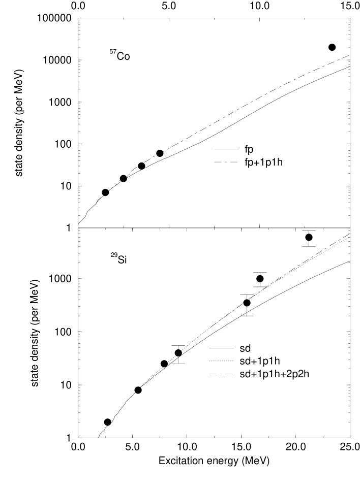
FIG. 3.: Comparison of experimental data of state densities for ⁵⁷Co and ²⁹Si against a sum of binomials. Error bars in the lower figure represent the spread in experimental data.

REFERENCES

- [1] S.E. Woosley, W.A. Fowler, J.A. Holmes and B.A. Zimmerman, At. Nucl. Data Tables 22, 371 (1978); F.-K. Thielemann, M. Arnould and J.W. Truran, Advances in Nuclear Astrophysics, eds. E. Vangioni-Flam et. al. p.525.
- [2] W. Dil, W. Schantl, H. Vonach and M. Uhl, Nucl. Phys. A 217, 269 (1973); J.R. Huizenga, H.K. Vonach, A.A. Katsanos, A.J. Gorski and C.J. Stephan, Phys. Rev. 182,1149 (1969); C.C. Lu, L.C. Vaz and J.R. Huizenga, Nucl. Phys. A 190, 229 (1972); A. Schiller, L. Bergholt, M. Guttormsen, E. Melby, J. Reststad and S. Seim, Nucl. Instum. Methods A 447, 498 (2000).
- [3] H.A. Bethe, Phys. Rev. 50, 332 (1936).
- [4] J.A. Holmes, S.E. Woosley, W.A. Fowler and B.A. Zimmerman, Atom. Data, Nucl. Data Tables 18, 305 (1976); J.J. Cowan, F.-K. Thielemann and J.W. Truran, Phys. Rep. 208, 267 (1991).
- [5] C.W. Johnson, S.E. Koonin, G.H. Lang and W.E. Ormand, Phys. Rev. Lett. 69, 3157 (1992).
- [6] D.J. Dean, S.E. Koonin, K. Langanke, P.B. Radha and Y. Alhassid, Phys. Rev. Lett. 74, 2909 (1995).
- [7] W. E. Ormand, Phys. Rev. C 56, R1678 (1997); H. Nakada and Y. Alhassid, Phys. Rev. Lett. 79 (1997) 2939; H. Nakada and Y. Alhassid, Phys. Lett. B 436, 231 (1998); J.A. White, S.E. Koonin and D.J. Dean, Phys. Rev. C 61, 034303 (2000).
- [8] K. K. Mon and J. B. French, Ann. Phys. 95, 90 (1975).
- [9] S. S. M. Wong, Nuclear Statistical Spectroscopy, Oxford Press (New York, 1986).
- [10] J.B. French and K.F. Ratcliff, Phys. Rev. C 3, 94 (1971)
- [11] S. Ayik and J.N. Ginocchio, Nucl. Phys. A 221, 285 (1974)
- [12] S. M. Grimes, S. D. Bloom, R. F. Hausman, Jr. and B. J. Dalton, Phys. Rev. C 19, 2378 (1979)
- [13] F. S. Chang and A. Zuker, Nucl. Phys. A 198, 417 (1972)
- [14] S. M. Grimes, S. D. Bloom, H. K. Vonach and R. F. Hausman, Jr., Phys. Rev. C 27, 2893 (1983)
- [15] Z. Pluhar and H. A. Weidenmüller, Phys. Rev. C 38 (1988) 1046.
- [16] D. J. Dean and S. E. Koonin, Phys. Rev. C 60, 054306 (1999).
- [17] A. P. Zuker, LANL archive nucl-th/9910002.
- [18] J. Nabi, C. W. Johnson, and W. E. Ormand, to be published.
- [19] B.H. Wildenthal, Prog. Part. Nucl. Phys. 11, 5 (1984).
- [20] B. A. Brown, A. Etchegoyen, and W. D. M. Rae, OXBASH, the Oxford University-Buenos Aires-MSU shell model code, Michigan State University Cyclotron Laboratory Report No. 524 (1985).
- [21] W. A. Richter, M. G. van der Merwe, R. E. Julies, and B. A. Brown, Nucl. Phys. A523, 325 (1990).
- [22] F.B. Bateman, S. M. Grimes, N. Boukharouba, V. Mishra, C.E. Brient, R.S. Pedroni, T.N. Massey and R.C. Haight, Phys. Rev. C 55, 133 (1997).
- [23] V. Mishra, N. Boukharouba, C.E. Brient, S. M. Grimes, and R.S. Perdoni, Phys. Rev. C 49, 750 (1994).
- [24] E. K. Wharburton, J. A. Becker, and B. A. Brown, Phys. Rev. C41, 1147 (1990).
- [25] T. Kuo and G. E. Brown, Nucl. Phys. A114, 241 (1968); A. Poves and A. P. Zuker, Phys. Rep. 70, 235 (1981).