Flow analysis from multiparticle azimuthal correlations

Abstract

We present a new method for analyzing directed and elliptic flow in heavy ion collisions. Unlike standard methods, it separates the contribution of flow to azimuthal correlations from contributions due to other effects. The separation relies on a cumulant expansion of multiparticle azimuthal correlations, and includes corrections for detector inefficiencies. This new method allows the measurement of the flow of identified particles in narrow phase-space regions, and can be used in every regime, from intermediate to ultrarelativistic energies.

I Introduction

In noncentral heavy ion collisions, it is possible to measure azimuthal distributions of outgoing particles with respect to the reaction plane. This is the so-called “flow analysis”, which is being actively studied over a wide range of colliding energies, from below 25 MeV per nucleon in the center-of-mass system [1] to above 60 GeV [2]. The main motivation for such studies is that anisotropies in the azimuthal distributions are likely to contain much information on the physics in the hot, dense central region of the collision (see [3, 4, 5] for reviews). In particular, they may provide a signature of the formation of a quark-gluon plasma at ultrarelativistic energies [6, 7]. Azimuthal distributions may also be of interest in connection with more exotic phenomena, such as the formation of disoriented chiral condensates [8, 9], or the study of parity and/or time-reversal violation[10]. Finally, the combination of flow analysis and two-particle interferometry yields a three-dimensional picture of the emitting source [11, 12, 13], as was shown recently at the Brookhaven Alternating Gradient Synchrotron (AGS) [14].

In this paper, we propose a new method to measure azimuthal distributions. As usual, they will be characterized by their Fourier coefficients [15]

$$v_{n}\equiv\langle e^{in(\phi-\Phi_{R})}\rangle=\langle\cos n(\phi-\Phi_{R})\rangle$$ (1)

where $\phi$ is the azimuthal angle of an outgoing particle measured in the laboratory coordinate system, $\Phi_{R}$ is the azimuth of the impact parameter (or reaction plane) and angular brackets denote a statistical average, over many events. The first two coefficients $v_{1}$ and $v_{2}$ are usually referred to as directed flow and elliptic flow, respectively. The $v_{n}$’s can be measured for various particle species, as a function of transverse momentum and/or rapidity: we refer to these detailed measurements as to “differential” flow, following [16]. In this paper, we also discuss global measurements of $v_{n}$, averaged over a large phase space region, typically corresponding to the acceptance of a detector. We call this “integrated” flow.

Since the reaction plane $\Phi_{R}$ cannot be measured directly, the only way to obtain the coefficients $v_{n}$ experimentally is to deduce them from the azimuthal correlations between the outgoing particles: the correlation between every particle and the reaction plane induces correlations among the particles (which we call hereafter the “flow correlations”), from which $v_{n}$ can be reconstructed. The method we propose here is based on a systematic analysis of multiparticle azimuthal correlations.

The most widely used method for the flow analysis is that initially proposed by Danielewicz and Odyniec [17] (see also [18, 19, 20] for further developments), which relies on azimuthal correlations between two “subevents”. It has recently been applied at intermediate energies in Darmstadt [1, 21], and at higher energies in Dubna [22, 23, 24], at the Brookhaven AGS [25, 26, 27], at the CERN Super Proton Synchrotron (SPS) [28, 29] and, finally, at the Brookhaven Relativistic Heavy Ion Collider (RHIC) [2]. An alternative, simpler method extracts flow from two-particle correlations [30] and is still in use, both at intermediate [31] and at ultrarelativistic energies [32, 33]. Both methods are more or less equivalent: correlating two subevents amounts to summing two-particle correlations. In these analyses, one usually assumes that the only sources of azimuthal correlations are flow and, when necessary, transverse momentum conservation [34].

However, we have shown in two papers [35, 36] that this assumption is no longer valid at SPS energies, where “direct”, nonflow two-particle correlations become of the same magnitude as the correlations due to flow. Even when nonflow correlations are a priori smaller than flow correlations, they must be taken into account in order to obtain accurate and reliable results. Some sources of nonflow correlations are well known. One can attempt to avoid them experimentally by appropriate cuts in phase space [2], or one can take them into account in the analysis [18], as was done for transverse momentum conservation [34, 36], for correlations from $\pi_{0}\to\gamma\gamma$ decays [37, 38], and for quantum correlations [35]. But there is no systematic way to separate the effects of flow from other effects at the level of two-particle correlations.

There have been several attempts in the past to go beyond two-particle correlations: analyses of the global event shape[39] allowed the first observations of collective flow at intermediate[40] and ultrarelativistic energies[41, 42], which were not biased by nonflow correlations. Multiparticle azimuthal correlations were also used in [43]. These methods are now considered obsolete because they apply only to the “integrated” flow, as defined above, whereas most of the recent analyses concentrate on the differential flow of identified particles, in particular kaons [26, 44], $\eta$ mesons [21], $\Lambda$ hyperons [27, 45], and antiprotons [46].

In recent papers [47, 48], we have shown for the first time that nonflow correlations can be removed systematically not only for integrated flow, but also in analyses of differential flow. However, a limitation of this method when measuring $v_{n}$ is the interference with higher harmonics ($v_{2n}$, $v_{3n}$, etc.). This interference may hinder the measurement of directed flow when elliptic flow is larger, which is likely to be the case at RHIC energies [49].

Here we present an improvement of this method, which is free from this limitation, and in many respects simpler. In particular, it no longer involves the event flow vector on which most analyses are based [17, 18, 47]. As in our previous method, we perform a cumulant expansion of multiparticle azimuthal correlations, which eliminates order by order nonflow correlations, and can be used even if the detector does not have full azimuthal coverage.

In Sec. II, we show how to construct the cumulants of multiparticle azimuthal correlations by means of a generating function. These cumulants allow us to reconstruct the integrated flow from the measured correlations. The method is extended to differential flow in Sec. III. The relation with other methods is discussed in Sec. IV. Results of Monte-Carlo simulations are presented in Sec. V. The most technical points are left to appendices: the construction of cumulants is explained in detail in Appendix A; interpolation formulas used to obtain the cumulants from the generating function are given in Appendix B; acceptance corrections, which extend the validity of the method to detectors with partial azimuthal coverage, are derived in Appendix C; finally, statistical errors on the flow values deduced from the cumulants are evaluated in Appendix D.

The essential improvement on our previous method is the use of a new generating function, defined in Sec. II B, which corrects the limitations encountered in [47]. These improvements are discussed in detail in Sec. IV and in Appendix A; they are seen clearly in the simulations presented in Sec. V. In addition, the detailed discussions of acceptance corrections (Appendix C) and statistical errors (Appendix D) are completely new, although they also apply to our previous method. Apart from these differences, most of the material discussed in Secs. II and III can be found in [47], although the present derivation is more transparent.

II Integrated flow

In Sec. II A, we illustrate with a few examples the principle of the cumulant expansion of multiparticle azimuthal correlations, and show how it can be used to perform flow measurements with a better sensitivity than the previous methods. Then we explain, in Sec. II B, how to perform this expansion in practice, by means of a generating function. In Sec. II C, we derive the relations between the cumulants and the flow $v_{n}$, integrated over some phase space region. Using cumulants to various orders, one thus obtains different estimates for $v_{n}$. The uncertainties associated with each estimate due to nonflow correlations and limited statistics, and the resulting optimal choice, are examined in Sec. II D. Finally, we discuss in Sec. II E the generalization of the previous subsections to different, optimal particle weights.

A Cumulants of multiparticle azimuthal correlations

We denote by $\phi_{j}$, with $j=1,\ldots,M$, the azimuthal angles of the particles seen in an event with multiplicity $M$, measured with respect to a fixed direction in the detector (this was denoted by $\bar{\phi}_{j}$ in [47]). In this paper, we shall be concerned with multiparticle azimuthal correlations, which we write generally in the form $\left\langle\exp[in(\phi_{1}+\cdots+\phi_{k}-\phi_{k+1}-\cdots-\phi_{k+l})]\right\rangle$, where $n$ is the Fourier harmonic under study ($n=1$ for directed flow, $n=2$ for elliptic flow), and the brackets indicate an average which is performed in two steps: first, one averages over all possible combinations of $k+l$ particles detected in the same event; then, one averages over all events.

Correlations between $k+l$ particles can be generally decomposed into a sum of terms involving correlations between a smaller number of particles. Consider for instance the measured two-particle azimuthal correlation $\left\langle e^{in(\phi_{1}-\phi_{2})}\right\rangle$. It can be written as

$$\left\langle e^{in(\phi_{1}-\phi_{2})}\right\rangle=\left\langle e^{in\phi_{1}}\right\rangle\left\langle e^{-in\phi_{2}}\right\rangle+\left\langle\!\!\left\langle e^{in(\phi_{1}-\phi_{2})}\right\rangle\!\!\right\rangle,$$ (2)

where $\left\langle\!\!\left\langle e^{in(\phi_{1}-\phi_{2})}\right\rangle\!\!\right\rangle$ is by definition the second order cumulant. To understand the physical meaning of this quantity, we first consider a detector whose acceptance is isotropic, i.e., which does not depend on $\phi$. Such a detector will be called a “perfect” detector. Then, the average $\left\langle e^{in\phi_{j}}\right\rangle$ vanishes by symmetry [since $\phi_{j}$ is measured in the laboratory, not with respect to the reaction plane, $\left\langle e^{in\phi_{j}}\right\rangle$ does not correspond to the flow $v_{n}$ defined in Eq. (1)]: the first term on the right-hand side (r.-h. s.) of Eq. (2) vanishes and the cumulant reduces to the measured two-particle correlation.

The relevance of the cumulant appears when considering the more realistic case of a detector with uneven acceptance. Then, the first term on the r.-h. s. of Eq. (2) can be nonvanishing. But the cumulant vanishes if $\phi_{1}$ and $\phi_{2}$ are uncorrelated. Thus the cumulant $\left\langle\!\!\left\langle e^{in(\phi_{1}-\phi_{2})}\right\rangle\!\!\right\rangle$ isolates the physical correlation, and disentangles it from trivial detector effects.

There are several physical contributions to the correlation $\left\langle\!\!\left\langle e^{in(\phi_{1}-\phi_{2})}\right\rangle\!\!\right\rangle$, which separate into flow and nonflow (or direct) correlations. When the source is isotropic (no flow), only direct correlations remain. They scale with the multiplicity $M$ like $1/M$ [35, 36], as can be easily understood when considering correlations between the decay products of a resonance: when a $\rho$ meson decays into two pions, momentum conservation induces an angular correlation of order unity between the decay pions; besides, the probability that two arbitrary pions seen in the detector result from the same $\rho$ decay scales with the total number of pions like $1/M$. All in all, the correlation between two arbitrary pions is of order $1/M$. If the source is not isotropic, flow, which is by definition a correlation between emitted particles and the reaction plane, generates azimuthal correlations between any two outgoing particles, and gives a contribution $v_{n}^{2}$ to the second-order cumulant, as will be explained in Sec. II C. One can measure the flow using the second-order cumulant if this contribution dominates over the nonflow contribution, i.e., if $v_{n}\gg 1/\sqrt{M}$ [35, 36]. This is the domain of validity of standard flow analyses, which are based on two-particle correlations.

Our main point is that through the construction of higher order cumulants, one can separate flow and nonflow correlations. To illustrate how this works, we consider for simplicity a perfect detector. Then, we decompose the measured four-particle correlation as follows:

$$\left\langle e^{in(\phi_{1}+\phi_{2}-\phi_{3}-\phi_{4})}\right\rangle=\left\langle e^{in(\phi_{1}-\phi_{3})}\right\rangle\left\langle e^{in(\phi_{2}-\phi_{4})}\right\rangle+\left\langle e^{in(\phi_{1}-\phi_{4})}\right\rangle\left\langle e^{in(\phi_{2}-\phi_{3})}\right\rangle+\left\langle\!\!\left\langle e^{in(\phi_{1}+\phi_{2}-\phi_{3}-\phi_{4})}\right\rangle\!\!\right\rangle.$$ (3)

If the particles are correlated pairwise, there are two possible combinations leading to a nonvanishing value for the left-hand side (l.-h. s.): the pairs can be either (1,3) and (2,4), or (1,4) and (2,3). This yields the first two terms in the right-hand side. The remaining term $\left\langle\!\!\left\langle e^{in(\phi_{1}+\phi_{2}-\phi_{3}-\phi_{4})}\right\rangle\!\!\right\rangle$, which is by definition the fourth-order cumulant, is thus insensitive to two-particle nonflow correlations. However, it may still be influenced by higher order nonflow correlations: if, for instance, a resonance decays into four particles, the resulting correlations between the reaction products do not factorize as in Eq. (3). We call such correlations “direct” four-particle correlations. Fortunately, their contribution to the fourth-order cumulant is very small: it scales with the multiplicity like $1/M^{3}$[47], while the measured correlation $\left\langle e^{in(\phi_{1}+\phi_{2}-\phi_{3}-\phi_{4})}\right\rangle$ is generally much larger, of order $1/M^{2}$ [the two-particle correlation terms in the r.-h. s. of Eq. (3) are of order $1/M$, as explained above]. On the other hand, flow yields a contribution $-v_{n}^{4}$ to the cumulant, as we shall see in Sec. II C. Therefore, the cumulant is dominated by the flow as soon as $v_{n}\gg 1/M^{3/4}$. This is a major improvement on two-particle correlations, which are limited by the much stronger constraint $v_{n}\gg 1/\sqrt{M}$.

Equation (3) can be rewritten

$$\left\langle e^{in(\phi_{1}+\phi_{2}-\phi_{3}-\phi_{4})}\right\rangle=2\,\left\langle e^{in(\phi_{1}-\phi_{3})}\right\rangle^{2}+\left\langle\!\!\left\langle e^{in(\phi_{1}+\phi_{2}-\phi_{3}-\phi_{4})}\right\rangle\!\!\right\rangle,$$ (4)

where we have used the symmetry between $\phi_{1}$ and $\phi_{2}$ (resp. $\phi_{3}$ and $\phi_{4}$). However, Eqs. (3) and (4) only hold for a perfect detector, therefore they are of little practical use. It is in fact possible to build an expression for the fourth-order cumulant which eliminates both detector effects and nonflow correlations, but this expression is very lengthy. This is the reason why we introduce a generating function of cumulants in Sec. II B. It will enable us to construct easily cumulants of arbitrary orders for arbitrary detectors.

More generally, the cumulant $\langle\!\langle\exp[in(\phi_{1}+\cdots+\phi_{k}-\phi_{k+1}-\cdots-\phi_{k+l})]\rangle\!\rangle$, which involves $k+l$ particles, is of order $M^{1-k-l}$ when there is no flow. It eliminates all nonflow correlations up to order $k+l-1$. Only direct correlations between $k+l$ particles remain. Cumulants with $k\not=l$ vanish for a perfect detector and are physically irrelevant. The interesting cumulants are the “diagonal” ones, with $k=l$, as in Eqs. (2) and (4). The contribution of flow to these cumulants, proportional to $v_{n}^{2k}$, will be evaluated precisely in Sec. II C. When this contribution dominates over the nonflow contribution, the measured cumulant yields an estimate of the value of $v_{n}$, which we denote by $v_{n}\{2k\}$, where $k>0$ is in principle arbitrary.

B Generating function

Cumulants can be expressed elegantly, and without assuming a perfect detector as in Eq. (4), using the formalism of generating functions. For each event, we define the real-valued function $G_{n}(z)$, which depends on the complex variable $z=x+iy$:

$$G_{n}(z) = \prod_{j=1}^{M}\left(1+{z^{*}e^{in\phi_{j}}+ze^{-in\phi_{j}}\over M}\right)$$ (5)

$$= \prod_{j=1}^{M}\left(1+{2\,x\cos(n\phi_{j})+2\,y\sin(n\phi_{j})\over M}\right),$$ (6)

where $z^{*}\equiv x-iy$ denotes the complex conjugate. This generating function can then be averaged over events with the same multiplicity $M$. We denote this statistical average by $\left\langle G_{n}(z)\right\rangle$. Its expansion in power series generates measured azimuthal correlations to all orders:

$$\left\langle G_{n}(z)\right\rangle = 1+{z\over M}\left\langle\sum_{j=1}^{M}e^{-in\phi_{j}}\right\rangle+{z^{*}\over M}\left\langle\sum_{j=1}^{M}e^{in\phi_{j}}\right\rangle$$ (8)

$$\qquad+{z^{2}\over M^{2}}\left\langle\sum_{j<k}e^{-in(\phi_{j}+\phi_{k})}\right\rangle+{z^{*2}\over M^{2}}\left\langle\sum_{j<k}e^{in(\phi_{j}+\phi_{k})}\right\rangle+{zz^{*}\over M^{2}}\left\langle\sum_{j\not=k}e^{in(\phi_{j}-\phi_{k})}\right\rangle+\cdots$$

$$= 1+z\left\langle e^{-in\phi_{1}}\right\rangle+z^{*}\left\langle e^{in\phi_{1}}\right\rangle+{M-1\over M}\left({z^{2}\over 2}\left\langle e^{-in(\phi_{1}+\phi_{2})}\right\rangle+{z^{*2}\over 2}\left\langle e^{in(\phi_{1}+\phi_{2})}\right\rangle+zz^{*}\left\langle e^{in(\phi_{1}-\phi_{2})}\right\rangle\right)+\cdots$$ (9)

where, the averages $\left\langle e^{in\phi_{1}}\right\rangle$, $\left\langle e^{in(\phi_{1}-\phi_{2})}\right\rangle$, etc. are defined as in Sec. II A. More generally, expanding $\left\langle G_{n}(z)\right\rangle$ to order $z^{*k}z^{l}$ yields, up to a numerical coefficient, the ($k+l$)-particle correlation $\left\langle\exp[in(\phi_{1}+\cdots+\phi_{k}-\phi_{k+1}-\cdots-\phi_{k+l})]\right\rangle$. The generating function $\left\langle G_{n}(z)\right\rangle$ thus contains all the information on measured multiparticle azimuthal correlations.

If the detector is perfect, the statistical average $\left\langle G_{n}(z)\right\rangle$ does not depend on the phase of $z$; it only depends on $|z|=\sqrt{x^{2}+y^{2}}$. To see this, one may note that changing $z$ into $z\,e^{in\alpha}$ in the generating function (5) amounts to shifting all angles by the same quantity $\phi_{j}\to\phi_{j}-\alpha$. Now, the probability for an event to occur is unchanged under a global rotation; therefore $\left\langle G_{n}(z)\right\rangle$ is unchanged under this rotation, hence the result. In this case, the only terms which remain in the power-series expansion are the isotropic terms, proportional to $z^{k}z^{*k}$, which involve only relative angles.

The generating function provides us with a way to obtain a compact expression for cumulants of arbitrary orders. We define the generating function of the cumulants ${\cal C}_{n}(z)$ by

$${\cal C}_{n}(z)\equiv M\left(\left\langle G_{n}(z)\right\rangle^{1/M}-1\right).$$ (10)

The expansion of this function in power series of $z$ and $z^{*}$ defines the cumulants:

$${\cal C}_{n}(z)\equiv\sum_{k,l}{z^{*k}z^{l}\over k!\,l!}\left\langle\!\!\left\langle e^{in(\phi_{1}+\cdots+\phi_{k}-\phi_{k+1}-\cdots-\phi_{k+l})}\right\rangle\!\!\right\rangle.$$ (11)

One easily checks that if the particles are uncorrelated, all the cumulants vanish beyond order one, i.e., for $k+l\geq 2$. Indeed, if all the $\phi_{j}$ in Eq. (5) are independent from each other, the mean value of the product is the product of the mean values, so that

$$\left\langle G_{n}(z)\right\rangle=\left(1+{z^{*}\left\langle e^{in\phi}\right\rangle+z\left\langle e^{-in\phi}\right\rangle\over M}\right)^{M}.$$ (12)

The generating function of cumulants, Eq. (10), then reduces to

$${\cal C}_{n}(z)=z^{*}\left\langle e^{in\phi}\right\rangle+z\left\langle e^{-in\phi}\right\rangle.$$ (13)

Comparing with Eq. (11), cumulants of order 2 and higher vanish when particles are uncorrelated, as expected.

The cumulant $\left\langle\!\!\left\langle e^{in(\phi_{1}-\phi_{2})}\right\rangle\!\!\right\rangle$ obtained when expanding Eqs. (10) and (11) to order $zz^{*}$ coincides with the second-order cumulant defined in Eq. (2) in the limit of large $M$ (see Appendix A). Expanding ${\cal C}_{n}(z)$ to order $z^{2}z^{*2}$, one obtains an expression for the cumulant $\left\langle\!\!\left\langle e^{in(\phi_{1}+\phi_{2}-\phi_{3}-\phi_{4})}\right\rangle\!\!\right\rangle$ which reduces to Eq. (4) for a perfect detector. But the expression derived from Eqs. (10) and (11) is still valid with an imperfect detector, while Eq. (4) is not.

As mentioned in Sec. II A, cumulants with $k\not=l$ vanish for a perfect detector, since the generating function ${\cal C}_{n}(z)$ in Eq. (11) depends only on $|z|$. The interesting cumulants are the diagonal terms with $k=l$, which are related to the flow. We denote them by $c_{n}\{2k\}$:

$$c_{n}\{2k\}\equiv\left\langle\!\!\left\langle e^{in(\phi_{1}+\cdots+\phi_{k}-\phi_{k+1}-\cdots-\phi_{2k})}\right\rangle\!\!\right\rangle.$$ (14)

In practice, expanding the generating function ${\cal C}_{n}(z)$ analytically is rather tedious beyond order 2. The simplest way to extract $c_{n}\{2k\}$ is to tabulate the generating function (10), and then compute numerically the coefficients of its power-series expansion, using interpolation formulas which can be found in Appendix B 1.

Finally, we have assumed here that the multiplicity $M$ is exactly the same for all events involved in the analysis. In practice, one performs the flow analysis for a class of events belonging to the same centrality interval, and $M$ fluctuates from one event to the other. That explains our introducing the factor $1/M$ in the definition of the generating function (5), as explained in more detail in Appendix A. The average over events $\left\langle G_{n}(z)\right\rangle$ then involves an average over $M$, and $M$ must be replaced by its average value $\left\langle M\right\rangle$ in the definition of the cumulants, Eq. (10). This, however, leads to errors, especially when the acceptance is bad (see Appendix A). This point will also be illustrated by the simulations presented in Sec. V. In order to avoid these effects, one may use only a randomly selected subset of the detected particles, with a fixed multiplicity $M$, to construct the generating function.

C Contribution of flow to the cumulants

Let us evaluate the contribution of flow to the cumulants $c_{n}\{2k\}$. For simplicity, we assume that the detector is perfect. The generalization to an uneven acceptance is performed in Appendix C 1. Under this assumption, one easily calculates the generating function $\left\langle G_{n}(z)\right\rangle$ and, from it, the values of the cumulants.

Let us call $\Phi_{R}$ the azimuthal angle of the reaction plane of a given event. The average over events can be performed in two steps: one first estimates the average over all events with the same $\Phi_{R}$; then one averages over $\Phi_{R}$. We denote by $\left\langle x|\Phi_{R}\right\rangle$ the average of a quantity $x$ for fixed $\Phi_{R}$. With this notation, the definition of $v_{n}$, Eq. (1), gives

$$\left\langle e^{in\phi_{j}}|\Phi_{R}\right\rangle=v_{n}\,e^{in\Phi_{R}}.$$ (15)

Neglecting for simplicity nonflow correlations between particles, we obtain from Eq. (5)

$$\left\langle G_{n}(z)|\Phi_{R}\right\rangle=\left(1+{z\,v_{n}\,e^{-in\Phi_{R}}+z^{*}v_{n}\,e^{in\Phi_{R}}\over M}\right)^{M}.$$ (16)

One must then average over $\Phi_{R}$:

$$\left\langle G_{n}(z)\right\rangle=\int_{0}^{2\pi}\left\langle G_{n}(z)|\Phi_{R}\right\rangle{d\Phi_{R}\over 2\pi}.$$ (17)

Inserting Eq. (16) in this expression, one obtains

$$\left\langle G_{n}(z)\right\rangle = \sum_{k=0}^{[M/2]}{M!\over(M-2k)!(k!)^{2}}\left({v_{n}\over M}\right)^{2k}|z|^{2k}$$ (18)

$$\simeq I_{0}(2\,v_{n}\,|z|),$$ (19)

where, in the last equation, we have assumed that $M$ is large, so that $M!/(M-2k)!=M^{2k}$ and one may extend the sum over $k$ to infinity. $I_{0}$ denotes the modified Bessel function of the first kind. The result depends only on $|z|$, as expected from the discussion in Sec. II C.

The generating function of the cumulants (10) now reads

$${\cal C}_{n}(z)\simeq M\left(I_{0}(2v_{n}|z|)^{1/M}-1\right)\simeq\ln I_{0}(2\,v_{n}\,|z|).$$ (20)

This equation can be expanded in power series. Comparing with Eq. (11), the cumulants with $k\not=l$ vanish, as expected for a perfect detector, while the diagonal cumulants $c_{n}\{2k\}$ defined by Eq. (14) are related to $v_{n}$. From the measured $c_{n}\{2k\}$, one thus obtains an estimate of $v_{n}$, which is denoted by $v_{n}\{2k\}$. The lowest order estimates are

$$v_{n}\{2\}^{2} \equiv c_{n}\{2\},$$ (22)

$$v_{n}\{4\}^{4} \equiv -c_{n}\{4\},$$ (23)

$$v_{n}\{6\}^{6} \equiv c_{n}\{6\}/4.$$ (24)

When the detector acceptance is far from isotropic, as is the case of the PHENIX detector at RHIC [33], which covers approximately half the range in azimuth, these relations no longer hold. The issue of acceptance corrections, discussed in detail in Appendix C, is more subtle than might be thought at first sight, for the following reason: when there is flow, the probability that a particle be detected depends on the orientation of the reaction plane $\Phi_{R}$ if the detector only has partial azimuthal coverage. Hence, if a fixed number of particles are emitted, the number of particles seen in the detector depends of $\Phi_{R}$. Reciprocally, for a fixed value of the multiplicity $M$ seen in the detector, the probability distribution of $\Phi_{R}$ is not uniform, which creates an important bias in the flow analysis. In the calculations of Appendix C 1, we assume the centrality selection is done by an independent detector (for instance a zero-degree calorimeter) which has (at least approximately) full azimuthal coverage, so that the distribution of $\Phi_{R}$ is uniform for the sample of events used in the flow analysis.

Under this assumption, one can derive general relations between the cumulants and the flow. It turns out that, in general, $c_{n}\{2k\}$ depends not only on $v_{n}$, but also on other harmonics $v_{p}$ with $p\not=n$. In order to obtain the corresponding relations, we introduce the acceptance function $A(\phi)$, which is the probability that a particle with azimuthal angle $\phi$ be detected. The Fourier coefficients of this acceptance function are

$$a_{p}\equiv\int_{0}^{2\pi}e^{-ip\phi}A(\phi){d\phi\over 2\pi}.$$ (25)

The relations between the cumulants $c_{n}\{2k\}$ and the estimates $v_{p}\{2k\}$ involve these coefficients. They are derived in Appendix C 1, to leading order in $v_{p}$. The results for directed flow and elliptic flow are given by Eqs. (C 1) and (C 1), respectively.

D Errors

We now examine the orders of magnitude of systematic errors, arising from unknown nonflow correlations, and statistical errors, due to the finite number of events available. More precisely, we estimate the difference $\delta v_{n}\{2k\}$ between the true integrated flow $v_{n}$ and its values reconstructed from the cumulants, $v_{n}\{2k\}$, defined in Eqs. (20). We show which value of $2k$ minimizes the total uncertainty.

As explained in Sec. II A, nonflow $2k$-particle correlations give a contribution of order $M^{1-2k}$ to the cumulant $c_{n}\{2k\}$. This is to be compared with the contribution of flow derived in Sec. II C, of order $v_{n}^{2k}$. We may thus write

$$v_{n}\{2k\}^{2k}-v_{n}^{2k}={\cal O}(M^{1-2k}),$$ (26)

which is an estimate of the systematic error $\delta v_{n}\{2k\}$ due to nonflow correlations. Obviously, flow can be measured only if $v_{n}^{2k}\gg M^{1-2k}$. For large orders $k\gg 1$, this condition becomes

$$v_{n}\gg 1/M,$$ (27)

which is a necessary condition for the flow to be measurable [47]. We believe there is no way to extract a flow of order $1/M$ or smaller.

In this paper, we always assume that condition (27) is fulfilled. If this is the case, the systematic error on $v_{n}$ given by Eq. (26), $\delta v_{n}\{2k\}\sim(Mv_{n})^{1-2k}$, becomes smaller and smaller as $k$ increases: thus one should construct cumulants of orders as high as possible.

One must also take into account the statistical error, due to the finite number of events $N_{\rm evts}$ available. The order of magnitude of statistical errors can easily be understood. The cumulant $c_{n}\{2k\}$ involves correlations between $2k$ particles belonging to the same event. There are roughly $M^{2k}$ ways (for large enough $M$) to choose $2k$ particles among the $M$ particles detected, and one averages over all possible combinations. Since this is done for all $N_{\rm evts}$ events, there is a total of $M^{2k}N_{\rm evts}$ subsets of $2k$ particles involved in the evaluation of the cumulants. The resulting statistical error is therefore

$$v_{n}\{2k\}^{2k}-v_{n}^{2k}={\cal O}\left({1\over\sqrt{M^{2k}N_{\rm evts}}}\right).$$ (28)

Unlike the systematic error, the statistical error generally increases with increasing cumulant order $2k$ (it may in fact decrease in some cases, but only slightly, see Appendix D 2). Therefore, the order $2k$ which gives the best compromise is that for which statistical and systematic errors are both of the same magnitude. Equating the right-hand sides of Eqs. (26) and (28), one obtains the optimal cumulant order [47]:

$$2\,k_{\rm opt}\simeq 2+\frac{\ln N_{\rm evts}}{\ln M}.$$ (29)

In most practical cases, the fourth-order cumulant ($2k=4$), that is, removing two-particle nonflow correlations, is to be preferred.

Statistical errors are discussed more thoroughly in Appendix D 2. There, we derive exact formulas for the standard deviations of the cumulants, and for their mutual correlations. Two regimes can be distinguished, depending on the value of the dimensionless parameter $\chi\equiv v_{n}\sqrt{M}$, which has been used previously as a measure of the reaction plane resolution [20]. If $\chi\ll 1$, the standard errors agree with the simple estimate (28), and different estimates $v_{n}\{2k\}$ and $v_{n}\{2l\}$ with $k\not=l$ are uncorrelated. If $\chi\gg 1$, on the other hand, they are strongly correlated and the standard error becomes

$$\delta(v_{n}\{2k\})_{\rm stat}={1\over\sqrt{2MN_{\rm evts}}},$$ (30)

independent of the order $2k$, and much larger than the estimate (28).

We also discuss in Appendix D 2 the non-Gaussian character of the fluctuations of the estimates $v_{n}\{2k\}$, due to their non-linear relations with the cumulants, Eqs. (20). In particular, statistical fluctuations may result in a “wrong” sign for the cumulant, in the sense that $v_{n}\{2k\}^{2k}$ defined by Eqs. (20) is negative. If this happens, the flow clearly cannot be estimated from the corresponding cumulant.

E Non-unit weights

In the definition of the generating function, Eq. (5), each particle was given the same weight. A more general form is

$$G_{n}(z)=\prod_{j=1}^{M}\left[1+{w_{j}\over M}\left(z^{*}e^{in\phi_{j}}+ze^{-in\phi_{j}}\right)\right].$$ (31)

The weight $w_{j}$ can be any arbitrary function of the rapidity $y$ of the particle, its transverse momentum $p_{T}$, its mass.

In order to obtain the highest accuracy on the flow measurement, $w_{j}$ should be chosen proportional to the flow itself, as shown in [47] (see also [50, 51]): the ideal weight is $w(p_{T},y)\propto v^{\prime}_{n}(p_{T},y)$, which is intuitively clear: one must give higher weights to particles with stronger flow. This is also the best choice if one uses the standard method, involving the determination of the reaction plane.

Ideally, the flow analysis should be performed twice: a first measurement of the flow can be done with reasonable guesses for the weights; measuring differential flow as a function of $y$ and $p_{T}$ for various particles (see Sec. III), the values obtained can be used as the new weights in a second, more accurate analysis. This is the procedure recently followed in [26].

A variety of weights have been used in analyses of the directed flow $v_{1}$. Since $v_{1}$ changes sign at midrapidity, the weight must be an odd function of the rapidity in the center-of-mass frame. Most often, the weight is simply the sign of $y$, with [17] or without [52] a gap at midrapidity. A linear dependence in $y$ was used in [53, 54, 55]. The latter choice is better, since $v_{1}$ is itself linear near midrapidity. The transverse momentum dependence of $w$ is most often linear, as in the original paper [17]. Unit weights, independent of $p_{T}$, are also widely used [21, 28, 56, 57]. They are convenient, because no particle identification is required. However, since $v_{1}$ is linear in $p_{T}$, (at least at low $p_{T}$ [51]), the original choice $w\propto p_{T}$ is likely to give more accurate results, although the opposite conclusion was reached in [56]. At intermediate energies, one can in addition choose a weight proportional to the mass of the particle, to take into account the fact that nuclear fragments flow more than protons [58, 59].

Unlike directed flow, elliptic flow is an even function of the center-of-mass rapidity: therefore the weights are usually chosen independent of rapidity. The weights are either independent of transverse momentum [2, 18, 28, 37, 38] or proportional to $p_{T}^{2}$ [41, 50, 60]. The latter choice is more appropriate if $p_{T}$ is measured, since $v_{2}$ is proportional to $p_{T}^{2}$ at low $p_{T}$ [51]. At ultrarelativistic energies, however, $v_{2}$ is almost linear in $p_{T}$ above 100 MeV [2, 61]. A better choice may be for instance $w(p_{T})=\sqrt{p_{T}^{2}+p_{0}^{2}}-p_{0}$, with $p_{0}\simeq 100$ MeV: this weight, quadratic at low $p_{T}$ and linear at high $p_{T}$, reproduces roughly the measured $p_{T}$ dependence of $v_{2}$.

With a non-unit weight $w$, the following modifications should be applied:

• In the relations between the cumulants and the flow, i.e., Eqs. (20) for integrated flow, Eqs. (41) and (III C) for differential flow, and the equations of Appendix C, $v_{n}$ now stands for $\left\langle we^{in(\phi-\Phi_{R})}\right\rangle$. Comparing with the previous definition, Eq. (1), the flow is now weighted by $w$, as can be expected from the definition of the generating function, Eq. (31).

• In the formulas giving the statistical errors, derived in Appendix D, one must in addition replace $M$ by $M/\left\langle w^{2}\right\rangle$. As a consequence, the resolution $\chi^{2}$ appearing in Eqs. (D24), (D27), (D44) and (D47) now stands for $\chi^{2}=M\left\langle wv_{n}\right\rangle^{2}/\left\langle w^{2}\right\rangle$.

• In the interpolation formulas of Appendix B, the value of $r_{0}$ [Eq. (B1)] should be scaled by the typical value of $w$, for instance by $\sqrt{\left\langle w^{2}\right\rangle}$.

III Differential flow

When one has measured the flow integrated over phase space, the next step is to move on to the “differential flow” analysis, i.e., the measurement of flow in a narrower phase space window. We call a particle belonging to the window of interest a “proton” (although it can be anything else). We denote by $\psi$ its azimuthal angle, and $v^{\prime}_{n}$ its flow harmonics (the so-called “differential flow”), $v^{\prime}_{n}\equiv\left\langle e^{in(\psi-\Phi_{R})}\right\rangle$. The particles used to estimate the integrated flow $v_{n}$ are named “pions”.

In order to measure the differential flow of the protons, we correlate their azimuth $\psi$ with the pion azimuths $\phi_{j}$. Once the integrated flow $v_{n}$ is known, one can reconstruct the differential flow $v^{\prime}_{n}$ from this correlation, and also higher harmonics $v^{\prime}_{2n}$, $v^{\prime}_{3n}$, etc. It follows that differential elliptic flow, $v^{\prime}_{2}$, can be reconstructed using either integrated directed flow or integrated elliptic flow. Following [18], we denote by $v^{\prime}_{p/n}$ the differential flow $v^{\prime}_{p}$ measured with respect to integrated flow $v_{n}$, where $p$ is a multiple of $n$. At intermediate energies, one usually measures $v^{\prime}_{2/1}$ [21] while $v^{\prime}_{2/2}$ is more accurate at ultrarelativistic energies where $v_{1}$ becomes very small [28].

The differential flow is reconstructed by taking the cumulants of azimuthal correlations between the proton and the pions. These are constructed in Sec. III A by means of an appropriate generating function. The subtraction of “autocorrelations”, in the case when the proton is one of the pions, is briefly discussed in Sec. III B. In Sec. III C, we derive the relations between the cumulants and the differential flow, $v^{\prime}_{p/n}$. As in the case of integrated flow, cumulants of different orders yield different estimates of $v^{\prime}_{p/n}$. The optimal choice is that which minimizes uncertainties, discussed in Sec. III D.

A Cumulants

To measure a proton differential flow $v^{\prime}_{p}$, we first construct a generating function of measured azimuthal correlations between the proton and pions. This function is the average value over all protons of $e^{ip\psi}G_{n}(z)$, where $G_{n}(z)$ is the generating function defined by Eq. (5), evaluated for the event where the proton belongs. Note that the average procedure is not exactly the same as when studying integrated flow. One must first average over the protons in a same event [i.e., with the same $G_{n}(z)$]; then, average over the events where there are “protons” (if the “proton” is some rare particle, or if the phase space window is small, there may be events without a proton).

Expanding in power series of $z$ and $z^{*}$, one obtains

$$\left\langle e^{ip\psi}G_{n}(z)\right\rangle=\left\langle e^{ip\psi}\right\rangle+z\left\langle e^{i(p\psi-n\phi_{1})}\right\rangle+z^{*}\left\langle e^{i(p\psi+n\phi_{1})}\right\rangle+\cdots$$ (32)

This generates measured azimuthal correlations between the proton and an arbitrary number of pions. The generating function of the cumulants is a complex-valued function of the complex variable $z$:

$${\cal D}_{p/n}(z)\equiv\frac{\left\langle e^{ip\psi}G_{n}(z)\right\rangle}{\left\langle G_{n}(z)\right\rangle},$$ (33)

where $\left\langle G(z)\right\rangle$ denotes an average over all events, as in Sec. II B. The cumulants are by definition the coefficients in the power-series expansion of this function:

$${\cal D}_{p/n}(z)\equiv\sum_{k,l}{z^{*k}z^{l}\over k!\,l!}\left\langle\!\!\left\langle e^{ip\psi+in(\phi_{1}+\cdots+\phi_{k}-\phi_{k+1}-\cdots-\phi_{k+l})}\right\rangle\!\!\right\rangle.$$ (34)

The physical significance of these cumulants is the same as for the cumulants used in the analysis of integrated flow. They eliminate detector effects and lower-order correlations, so that only the direct correlation between $k+l$ pions and the proton, of order $M^{-k-l}$, and the correlation due to flow remain. If the proton is not correlated with the pions, for instance, Eq. (33) gives ${\cal D}_{p/n}(z)=\left\langle e^{ip\psi}\right\rangle$, independent of $z$, and all cumulants with $k+l\geq 1$ vanish according to Eq. (34). In the more general case when there are correlations, expanding Eq. (33) to order $z$ and identifying with Eq. (34), one obtains

$$\left\langle\!\!\left\langle e^{i(p\psi-n\phi_{1})}\right\rangle\!\!\right\rangle\equiv\left\langle e^{i(p\psi-n\phi_{1})}\right\rangle-\left\langle e^{ip\psi}\right\rangle\left\langle e^{-in\phi_{1}}\right\rangle.$$ (35)

This cumulant is analogous to Eq. (2), and can be interpreted in the same way.

If the detectors used to measure protons and pions are perfect, simplifications occur: first, the cumulants defined in Eq. (34) are real. To show this, we use the property that if the detector is perfect, the probability that an event occur is unchanged when one reverses the sign of all azimuthal angles (i.e., $\psi\to-\psi$ and $\phi_{j}\to-\phi_{j}$), therefore ${\cal D}_{p/n}(z)$ is unchanged under this transformation. Now, the transformation $\phi_{j}\to-\phi_{j}$ amounts to changing $z$ into $z^{*}$ in $G_{n}(z)$, according to Eq. (5). Thus, Eq. (33) can also be written ${\cal D}_{p/n}(z)=\left\langle e^{-ip\psi}G_{n}(z^{*})\right\rangle/\left\langle G_{n}(z^{*})\right\rangle$. Comparing with the original definition, Eq. (33), $z$ has been changed to $z^{*}$ and $\psi$ to $-\psi$. Now, changing $\psi$ to $-\psi$ in Eq. (33) amounts to taking the complex conjugate of ${\cal D}_{p/n}(z)$, since $G_{n}(z)$ is real. One finally obtains ${\cal D}_{p/n}(z)={\cal D}^{*}_{p/n}(z^{*})$, from which one easily deduces that the coefficients in the expansion (34) are real. They are in general complex with a realistic detector, but only the real part is relevant.

Furthermore, most cumulants vanish if the detector is perfect. In order to see this property, we shift all angles by the same quantity $\alpha$, which does not change the probability of the event. The angles of the pions are changed to $\phi_{j}-\alpha$, which amounts to changing $z$ into $ze^{in\alpha}$ in $G_{n}(z)$, as explained in Sec. II B. Similarly, the angle of the proton $\psi$ is changed to $\psi\to\psi-\alpha$, so that $e^{ip\psi}G_{n}(z)$ becomes $e^{ip\psi}e^{-ip\alpha}G_{n}(ze^{in\alpha})$. Averaging over $\alpha$ gives 0 unless $p$ is a multiple of $n$, which is the case we are interested in. Writing $p=mn$, the only terms which remain in the power series expansion of $\left\langle e^{ip\psi}G_{n}(z)\right\rangle$ are the terms in $z^{*k}z^{k+m}$. To obtain the generating function of cumulants ${\cal D}_{p/n}(z)$, one must divide by $\left\langle G_{n}(z)\right\rangle$. Since this quantity depends only on $|z|$, as explained in Sec. II B, the only nonvanishing cumulants in Eq. (34) are those with $l=k+m$. Other cumulants are physically irrelevant.

Finally, the relevant quantities are

$$d_{mn/n}\{2k+m+1\}\equiv{\Re}\left[\left\langle\!\!\left\langle e^{in(m\psi+\phi_{1}+...+\phi_{k}-\phi_{k+1}-...-\phi_{2k+m})}\right\rangle\!\!\right\rangle\right].$$ (36)

where ${\Re}$ denotes the real part, and the notation $\{2k+m+1\}$ means that the cumulant involves correlations between $2k+m+1$ particles (one proton and $2k+m$ pions).

When there is no flow, $d_{mn/n}\{2k+m+1\}$ is of order $M^{-2k-m}$. Flow gives a contribution to this cumulant, proportional to $v^{\prime}_{p}v_{n}^{2k+m}$, which is calculated in Sec. III C. If this is the dominant contribution, one obtains an estimate of the differential flow $v^{\prime}_{p}$ from the cumulant $d_{p/n}\{2k+m+1\}$, using a previously determined value of the integrated flow $v_{n}$. This estimate will be denoted by $v^{\prime}_{p/n}\{2k+m+1\}$.

Analytical expressions of higher order cumulants, deduced from Eq. (34), are lengthy. As in the case of integrated flow, the simplest way to extract them consists in tabulating the generating function ${\cal D}_{mn/n}(z)$, and then computing numerically the coefficients of its power-series expansion, through interpolation formulas which are given in Appendix C 2.

B Autocorrelations

When studying the azimuthal correlations between the “proton” and the “pions”, the “proton” must not be one of the “pions”, otherwise trivial autocorrelations would appear. This problem is well known in the standard flow analysis [17]: in order to avoid it, one excludes the particle under study (the “proton”) from the definition of the flow vector used to estimate the reaction plane, which usually involves all the other particles (the “pions”). Here, if the proton is one of the pions, one simply removes its contribution by dividing $G_{n}(z)$ by $1+(z^{*}e^{in\psi}+ze^{-in\psi})/M$ in the numerator of Eq. (33). The generalization of this procedure to non-unit weights is straightforward.

C Contribution of flow to the cumulants

Let us now calculate the contribution of flow to the cumulants $d_{mn/n}\{2k+m+1\}$. As in Sec. II C, we neglect nonflow correlations and assume a perfect detector for simplicity. Under these assumptions, we can compute the generating function of the cumulants ${\cal D}_{p/n}(z)$. We first average over all events with a fixed orientation of the reaction plane $\Phi_{R}$, and over the protons in each single event:

$$\left\langle e^{ip\psi}|\Phi_{R}\right\rangle=v^{\prime}_{p}e^{ip\Phi_{R}}.$$ (37)

Hence, Eq. (33) becomes

$${\cal D}_{p/n}(z)=\frac{\int_{0}^{2\pi}e^{ip\Phi_{R}}\left\langle G_{n}(z)|\Phi_{R}\right\rangle d\Phi_{R}/2\pi}{\left\langle G_{n}(z)\right\rangle}\,v^{\prime}_{p},$$ (38)

where the denominator is given by Eq. (18), and $\left\langle G_{n}(z)|\Phi_{R}\right\rangle$ by Eq. (16). The numerator vanishes unless $p$ is a multiple of $n$, i.e., $p=mn$ with $m$ integer. Integrating over $\Phi_{R}$, one then obtains:

$$\int_{0}^{2\pi}e^{imn\Phi_{R}}\left\langle G_{n}(z)|\Phi_{R}\right\rangle{d\Phi_{R}\over 2\pi} = \sum_{k=0}^{[(M+m)/2]}{M!\over(M-m-2k)!\,k!\,(2k+m)!}\left({v_{n}\over M}\right)^{2k+m}z^{*k}z^{k+m}$$ (39)

$$\simeq I_{m}(2\,v_{n}\,|z|)\left(\frac{z}{|z|}\right)^{m},$$ (40)

where, in the last identity, we have assumed that $M$ is large, so that $M!/(M-m-2k)!\simeq M^{2k+m}$ and we may extend the sum over $k$ to infinity. Equation (38) gives

$${\cal D}_{mn/n}(z)=\frac{I_{m}(2|z|v_{n})}{I_{0}(2|z|v_{n})}\,\left(\frac{z}{|z|}\right)^{m}v^{\prime}_{mn}.$$ (41)

This equation can be expanded in power series of $z$ and $z^{*}$. The coefficients of the power-series expansion are real, as expected from the discussion in Sec. III A. Comparing with Eq. (34), cumulants with $l\not=k+m$ vanish, which was also expected; cumulants with $l=k+m$, which are the $d_{mn/n}\{2k+m+1\}$ introduced in Eq. (36), are proportional to $v^{\prime}_{mn}$. We thus obtain estimates of the differential flow $v^{\prime}_{mn}$, which we denote by $v^{\prime}_{mn/n}\{2k+m+1\}$, from the measured cumulants. For $m=1$ (the proton is correlated with pions in the same flow harmonic) these estimates are given by

$$v^{\prime}_{n/n}\{2\} \equiv d_{n/n}\{2\}/v_{n}$$ (43)

$$v^{\prime}_{n/n}\{4\} \equiv -d_{n/n}\{4\}/v_{n}^{3},$$ (44)

while for $m=2$ (useful when measuring differential elliptic flow $v^{\prime}_{2}$ with respect to the integrated directed flow $v_{1}$)

$$v^{\prime}_{2n/n}\{3\} \equiv d_{2n/n}\{3\}/v_{n}^{2}$$ (46)

$$v^{\prime}_{2n/n}\{5\} \equiv -d_{2n/n}\{5\}/(2\,v_{n}^{4}).$$ (47)

As in the case of integrated flow, a non-perfect acceptance may induce interference between the various harmonics $v^{\prime}_{n}$, $v^{\prime}_{2n}$, etc., modifying Eqs. (41) and (III C). The corresponding relations between the cumulants and the flow are derived in Appendix C 2. We have taken into account the possibility that integrated and differential flows may be measured using detectors with different azimuthal coverages, which is often the case in practice (see for instance [21]). In particular, if the detector used for integrated flow is perfect, we show that no correction is required for $v^{\prime}_{n}$, whatever the detector used for differential flow may be, which is intuitively obvious: the only difference when using a smaller detector for the reconstruction of differential flow is then a loss in “proton” multiplicity, resulting in higher statistical errors, which we now discuss.

D Errors

As in Sec. II D, we now evaluate the contributions of nonflow correlations and statistical fluctuations to the cumulants. This will allow us to determine the optimal cumulant order to be used, which minimizes the total uncertainty on $v^{\prime}_{p}$.

As discussed in Sec. III A, nonflow correlations give an unknown contribution of order $M^{-2k-m}$ to the cumulant $d_{p/n}\{2k+m+1\}$, which must be compared with the contribution of flow, proportional to $v^{\prime}_{mn}\{2k+m+1\}\,v_{n}^{2k+m}$ as shown in Sec. III C. The systematic error on $v^{\prime}_{mn/n}$ thus reads

$$v^{\prime}_{mn/n}\{2k+m+1\}-v^{\prime}_{mn/n}={\cal O}\left((Mv_{n})^{-2k-m}\right).$$ (48)

According to Eq. (27), this systematic error becomes smaller and smaller as $k$ increases: the same behavior was observed for the systematic error on the integrated flow in Sec. II D.

The order of magnitude of statistical errors can be estimated in the same way as for integrated flow. The cumulant $d_{p/n}\{2k+m+1\}$ involves correlations of the proton with $2k+m$ pions belonging to the same event. There are roughly $M^{2k+m}$ ways (if $M$ is large enough) to choose $2k+m$ pions among $M$. Denoting by $N^{\prime}$ the total number of protons involved in the analysis, there is a total of $M^{2k+m}N^{\prime}$ subsets of particles involved in evaluating the cumulants. The resulting statistical error is therefore

$$v^{\prime}_{mn/n}\{2k+m+1\}-v^{\prime}_{mn/n}={\cal O}\left({1\over\sqrt{M^{2k+m}N^{\prime}}}\right){1\over v_{n}^{2k+m}}.$$ (49)

As was the case for integrated flow, the statistical error usually increases with the order of the cumulant, while the systematic error decreases. Therefore, the cumulant order which gives the best compromise is that for which statistical and systematic errors are both of the same order of magnitude. Equating the right-hand sides of Eqs. (48) and (49), one obtains the optimal cumulant order [47]:

$$(2\,k+m+1)_{\rm opt}\simeq 1+\frac{\ln N^{\prime}}{\ln M}.$$ (50)

Statistical errors are evaluated in detail in Appendix D 3. We show that the simple estimate (49) is correct only if $\chi\equiv v_{n}\sqrt{M}\ll 1$. In this limit, different estimates $v^{\prime}_{mn/n}\{2k+m+1\}$ and $v^{\prime}_{mn/n}\{2l+m+1\}$ with $k\not=l$ are uncorrelated. When $\chi\gg 1$, the correlation becomes strong and the standard error is approximately

$$\delta(v^{\prime}_{mn/n}\{2k+m+1\})_{\rm stat}={1\over\sqrt{2N^{\prime}}},$$ (51)

independent of the order $2k+m+1$, and much larger than the estimate (49).

IV Comparison with other methods

The method proposed in this paper is closely related to our first cumulant-based method [47], since it is aimed at correcting some of the latter’s limitations. This is discussed in Sec. IV A. Then, in Sec. IV B, we compare our method with the two-particle correlation technique [30] and with the subevent method [17, 18].

A Comparison with our previous method

The cumulant expansion proposed in [47] was based on the flow vector rather than on particles themselves. The flow vector is defined for each event by [17, 18]

$$Q_{n}\equiv\frac{1}{\sqrt{M}}\sum_{j=1}^{M}e^{in\phi_{j}}.$$ (52)

A generating function was then defined:

$${\cal G}_{0}(z)\equiv\left\langle e^{zQ_{n}^{*}+z^{*}Q_{n}}\right\rangle.$$ (53)

The expansion of this generating function generates all the moments of the distribution of $Q$, that is, $\langle Q^{k}Q^{*l}\rangle$. One easily shows that ${\cal G}_{0}(z)$ is closely related to the generating function used in the present paper. Using the identity

$$1+{z^{*}e^{in\phi_{j}}+ze^{-in\phi_{j}}\over M}\simeq\exp\left({z^{*}e^{in\phi_{j}}+ze^{-in\phi_{j}}\over M}\right),$$ (54)

valid for large $M$, we may rewrite the generating function (5) as

$$G_{n}(z) \simeq \exp\left(z^{*}\sum_{j=1}^{M}e^{in\phi_{j}}+z\sum_{j=1}^{M}e^{-in\phi_{j}}\right)$$ (55)

$$= \exp\left({z^{*}\over\sqrt{M}}Q_{n}+{z\over\sqrt{M}}Q_{n}^{*}\right).$$ (56)

Thus the average over events $\left\langle G_{n}(z)\right\rangle$ coincides with ${\cal G}_{0}(z/\sqrt{M})$. This shows that both methods are equivalent in the large $M$ limit, up to a rescaling of the variable $z$.

The difference between the two approaches can be easily understood by expanding the two generating functions in powers of $z$ and $z^{*}$. To second order, for instance, Eqs. (52) and (53) give

$${\cal G}_{0}(z)=\cdots+{zz^{*}\over M}\left\langle\sum_{j,k}e^{in(\phi_{j}-\phi_{k})}\right\rangle+{z^{2}\over 2M}\left\langle\sum_{j,k}e^{-in(\phi_{j}+\phi_{k})}\right\rangle+{z^{*2}\over 2M}\left\langle\sum_{j,k}e^{in(\phi_{j}+\phi_{k})}\right\rangle+\cdots$$ (57)

while our new generating function gives (see Eq.(8))

$$\left\langle G_{n}(z)\right\rangle=\cdots+{zz^{*}\over M^{2}}\left\langle\sum_{j\not=k}e^{in(\phi_{j}-\phi_{k})}\right\rangle+{z^{2}\over 2M^{2}}\left\langle\sum_{j\not=k}e^{-in(\phi_{j}+\phi_{k})}\right\rangle+{z^{*2}\over 2M^{2}}\left\langle\sum_{j\not=k}e^{in(\phi_{j}+\phi_{k})}\right\rangle+\cdots$$ (58)

The essential difference is the restriction $j\not=k$ in the sums: our new method is free from the autocorrelations corresponding to the terms with $j=k$ in Eq. (57). This remains true to higher orders in $z$ and $z^{*}$.

Autocorrelations have two effects: in the first term of Eq. (57), they give a constant, trivial contribution which must then be removed. This fixes the choice of the weight $1/\sqrt{M}$ in the definition of the flow vector, Eq. (52). With another weight, the contribution of autocorrelations would depend on $M$, and it would not be easy to subtract them when $M$ is allowed to fluctuate. With the new generating function, we are free to choose another weight, and we show in Appendix A that the weight $1/M$ [Eq. (5)] gives more accurate results when $M$ is allowed to fluctuate.

In the second and third terms of Eq. (57), autocorrelations create terms in $e^{\pm 2in\phi_{j}}$ which interfere with higher harmonics. This was the main limitation of the method exposed in [47]. Eliminating all autocorrelations represents a major improvement. In particular, our method should enable to measure directed flow at RHIC, if any.

Finally, let us comment on our definition of the cumulants through the generating function ${\cal C}_{n}(z)$ in Eq. (10). This definition ensures that cumulants of order 2 and higher vanish if particles are uncorrelated [see the discussion following Eq. (11)]. In the limit when $M$ is large, one recovers ${\cal C}_{n}(z)=\ln\left\langle G_{n}(z)\right\rangle$, in agreement with the standard definition of cumulants in probability theory [62], and with the definition we adopted in [47].

B Comparison with standard methods

In [30], it was proposed to analyse flow using two-particle azimuthal correlations. More specifically, one defines by $P_{\rm corr}(\Delta\phi)$ [resp. $P_{\rm uncor}(\Delta\phi)$] the distribution of the relative angle $\Delta\phi\equiv\phi_{1}-\phi_{2}$, where $\phi_{1}$ and $\phi_{2}$ are any two particles belonging to the same event (resp. belonging to two different events). One then constructs the ratio

$$C(\Delta\phi)\equiv\frac{P_{\rm corr}(\Delta\phi)}{P_{\rm uncorr}(\Delta\phi)},$$ (59)

This so-called “mixed event” technique enables the extraction of the physical correlations between the particles, eliminating the effects of an uneven detector acceptance. Neglecting nonflow correlations, one has in general

$$C(\Delta\phi)=\sum_{n=-\infty}^{+\infty}v_{n}^{2}e^{in\Delta\phi},$$ (60)

so that the Fourier expansion of the measured correlation function $C(\Delta\phi)$ simply yields the integrated flow $v_{n}$. Similarly, if one replaces $\phi_{1}$ with the azimuthal angle $\psi$ of a particle in a narrow phase space window, $v_{n}^{2}$ in Eq. (60) is replaced with $v^{\prime}_{n}v_{n}$, where $v^{\prime}_{n}$ is the differential flow of the particle of interest.

The values of $v_{n}$ and $v^{\prime}_{n}$ obtained with this method coincide with the values we obtain from the cumulant of order 2, which are denoted by $v_{n}\{2\}$ and $v^{\prime}_{n}\{2\}$ in this paper; while we do not need mixed events, we must apply correction factors to our reconstructed $v_{n}\{2\}$ and $v^{\prime}_{n}\{2\}$ if the detector does not have full azimuthal coverage, as explained at the end of Secs. II C and III C. With the mixed-event technique, this correction is not required [33].

The essential limitation of the two-particle correlation technique is that it is not possible to separate flow and nonflow correlations: therefore the results may be strongly biased by nonflow correlations, which are eliminated in our method by the construction of higher order cumulants.

The same limitation applies to the much more widely used subevent method [17]. This methods involves two steps: in each event, one constructs the flow vector (52) to estimate the orientation of the reaction plane $\Phi_{R}$, and a study of the azimuthal correlation between the flow vectors of two randomly chosen “subevents” yields the accuracy of this estimate (the so-called “reaction plane resolution”). This first step amounts to measuring the integrated flow. Then, in order to measure differential flow, one studies the azimuthal correlation between a single particle and the flow vector. Since the latter involves a summation over many particles, the correlation between a single particle and the flow vector is much stronger than the correlation between two single particles, which is probably the reason why this method is used so often. However, the relative weights of nonflow and flow correlations is the same [47] as in the much simpler two-particle correlation technique discussed above, so that both suffer from the same limitations.

Flow and nonflow correlations could in fact be distinguished in the subevent method, through a more detailed study of the azimuthal correlation between subevents. Indeed, flow and nonflow correlations yield a different shape of the distribution of the relative azimuthal angle $\Delta\Phi$ between subevents, as shown in [63]. If correlations are only due to flow, then the distribution of $\Delta\Phi$ is universal, and depends only on the resolution $\chi\equiv v_{n}\sqrt{M}$ which characterizes the reaction plane resolution [19]. A comparison of the calculated distribution with experimental data was recently done at energies of 250 MeV per nucleon [1]. The agreement is perfect, which shows that the observed correlations are dominated by flow at these energies. To our knowledge, no such comparison has been carried out so far at ultrarelativistic energies.

V Results of Monte-Carlo simulations

We have performed various Monte-Carlo simulations to check the validity of the procedures explained in this paper. In each simulation, $N_{\rm evts}$ events are simulated; in a given event, the reaction plane $\Phi_{R}$ is chosen randomly, then “pions” and “protons” are generated according to the respective distributions

$${dN\over d\phi}\propto 1+2v_{1}\cos(\phi-\Phi_{R})+2v_{2}\cos\left(2(\phi-\Phi_{R})\right)$$ (61)

and

$${dN^{\prime}\over d\psi}\propto 1+2v^{\prime}_{1}\cos(\psi-\Phi_{R})+2v^{\prime}_{2}\cos\left(2(\psi-\Phi_{R})\right)$$ (62)

respectively. We then reconstruct the integrated (Sec. V A) and differential (Sec. V B) flows following the procedures exposed in Secs. II and III.

A Integrated flow

In the first set of simulations, we generated $N_{\rm evts}=10^{5}$ events with $M=200$ pions emitted with an integrated elliptic flow $v_{2}=6\%$, which we then tried to reconstruct. No integrated directed flow was simulated. We first assumed a perfect detector. The optimal cumulant order, defined by Eq. (29), is $2k_{\rm opt}=4.2$. The estimate $v_{2}\{4\}$ derived from the fourth-order cumulant is thus likely to give the best compromise between systematic and statistical errors, but we also calculated the estimates $v_{2}\{2\}$ and $v_{2}\{6\}$.

	$v_{2}\{2\}$	$v_{2}\{4\}$	$v_{2}\{6\}$
full acceptance, $M=200$	$6.01\pm 0.02$	$6.03\pm 0.04$	$6.08\pm 0.05$
full acceptance, $150<M<250$	$6.01\pm 0.02$	$6.11\pm 0.04$	$6.13\pm 0.05$
nonflow correlations, $M=200$	$9.21\pm 0.02$	$6.16\pm 0.04$	$6.19\pm 0.05$
“bow tie” acceptance, $M=100$	$5.99\pm 0.04$	$6.09\pm 0.12$	$6.34{\matrix{+0.19\cr-0.22}}$
“bow tie” acceptance, $75<M<125$	$5.85\pm 0.04$	$5.40\pm 0.12$	$5.74{\matrix{+0.19\cr-0.22}}$

TABLE I.: Reconstruction of integrated elliptic flow. $N_{\rm evts}=10^{5}$ events with $v_{1}=0$ and $v_{2}=6\%$ were generated in each simulation. The three columns give the values of $v_{2}$, in $\%$, reconstructed using cumulants to order $2$, $4$, and $6$, respectively.

The results are presented in Table I. The error bars are statistical only. They are asymmetric for $v_{2}\{6\}$: this reflects the fact that the statistical fluctuations of $v_{n}\{2k\}$ are not Gaussian when the error is large, as explained in Appendix D 2. When working with a fixed multiplicity $M=200$, the reconstructed values coincide with the theoretical value within expected statistical errors. Note that the statistical error on $v_{2}\{6\}$ is only slightly larger than that on $v_{2}\{4\}$ in this case. When the multiplicity $M$ is randomly chosen between 150 and 250, the reconstructed flow deviates from the theoretical value by more than two standard deviations, but the accuracy is still good, and moreover the statistical errors were calculated assuming a fixed detected multiplicity, while the real errors are probably larger.

In order to check the ability of our method to eliminate two-particle nonflow correlations, the latter were simulated by emitting particles in pairs, where both particles in a pair have the same azimuthal angle. $100$ pairs were emitted in each event, resulting in a multiplicity $M=200$. The reconstructed value with the cumulant of order 2 , i.e., without removing two-particle nonflow correlations, is 50% too large; the standard methods would give similar results. On the other hand, the values obtained using higher order cumulants are much closer to the theoretical value; they are beyond statistical error bars, but this is not surprising since error bars were calculated assuming $M=200$ independent particles, while the effective multiplicity here is rather 100, which results in larger fluctuations.

In summary, the results obtained so far show that $v_{2}\{4\}$ is to be preferred here: the statistical error on $v_{2}\{6\}$ is (slightly) larger, while nonflow correlations may give a large, uncontrolled, contribution to $v_{2}\{2\}$.

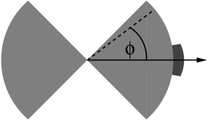
FIG. 1.: Schematic picture of the PHENIX detector at RHIC. The shaded area indicates the azimuthal coverage of the detector, while the darker area at the right of the figure corresponds to a small time-of-flight detector with an extension of $45^{\circ}$, which can be used to measure the differential flow of identified particles.

To test the validity of our acceptance corrections, we then did simulations with the “bow-tie” detector schematically represented in Fig. 1, which mimics the azimuthal acceptance of the PHENIX detector [33]: particles are detected only within two quadrants of $90$ degrees each, with $100\%$ efficiency. Since only half the particles are detected with this detector, the value of $M$ chosen in this simulation was half the value chosen above for a perfect detector. The optimal cumulant order is now $2k_{\rm opt}=4.5$, so that the fourth-order cumulant is still to be preferred. Since the azimuthal coverage is only partial, Eqs. (20) relating the cumulant to the flow are no longer valid. In the case of elliptic flow, they are replaced by Eqs. (C 1). These formulas involve the Fourier coefficients $a_{p}$ of the acceptance function, defined by Eq. (25). With the acceptance depicted in Fig. 1, a simple calculation gives $a_{2}=2/\pi$ and $a_{1}=a_{3}=a_{4}=0$. Inserting these values into Eqs. (C 1), one finds

$$c_{2}\{2\} \simeq 0.518\,v_{2}\{2\}^{2},$$ (63)

$$c_{2}\{4\} \simeq -0.384\,v_{2}\{4\}^{4}.$$ (64)

An interesting feature of this bow-tie acceptance is that there is no interference between $v_{1}$ and $v_{2}$, because all $a_{p}$ with odd $p$ vanish. However, this is not the case in general (see Appendix C). The results are given in Table I. Note that the estimate of statistical errors was done assuming a full acceptance, so they may be underestimated here. When the multiplicity $M$ is fixed, the reconstructed values agree with the theoretical values within eror bars. If the acceptance correction had not been applied, the reconstructed values would be below $5\%$.

If $M$ is allowed to fluctuate, the discrepancy between reconstructed and theoretical values is much larger than statistical errors, and also much larger than in the case of a full acceptance. As explained in Appendix A, a fluctuation $\delta M$ in multiplicity induces some errors, which scale like $\delta M^{2}$ and are comparatively larger when the acceptance is not good. In order to avoid this effect, the analysis can be done by selecting randomly a subset of the detected particles, with fixed multiplicity, as explained at the end of Sec. II B.

	$v_{2}=0$	$v_{2}=6\,\%$
full acceptance, $M=200$	$2.01{\matrix{+0.21\cr-0.32}}$	$2.19{\matrix{+0.21\cr-0.32}}$
“bow-tie” acceptance, $M=200$	$1.87{\matrix{+0.21\cr-0.32}}$	$1.88{\matrix{+0.21\cr-0.32}}$

TABLE II.: Reconstruction of a theoretical directed flow $v_{1}=2\,\%$. $N_{\rm evts}=5\times 10^{5}$ events were generated in each simulation, with $M=200$ detected particles in each event. The table gives the values of $v_{1}\{4\}$ in $\%$.

We then performed a second set of simulations, with both directed and elliptic flow, in order to test possible interferences between the two. Such uncontrolled interferences were the main limitation of our previous cumulant method [47], but are avoided here, as explained in Sec. IV A. Inteference of a different kind may in fact still occur when the detector has partial azimuthal coverage, as explained in Appendix C 1, but they are under control. Events were generated with a small directed flow $v_{1}=2\%$, and with an elliptic flow $v_{2}=0$ or $v_{2}=6\%$. The goal was to reconstruct $v_{1}$. Since $2\%$ is a very small value, a larger number of events were generated than in the previous set of simulations. With the values of $N_{\rm evts}$ and $M$ given in Table II, the optimal cumulant order is still 4: all the results presented in Table II are reconstructed from the fourth-order cumulant. In the case of the bow-tie acceptance, the relation between $v_{1}\{4\}$ and the cumulant, Eq. (23), must be replaced with (C10), which gives

$$c_{1}\{4\}\simeq-2.785\,v_{1}\{4\}^{4}.$$ (65)

The reconstructed value of $v_{1}$ is always compatible with the theoretical value $v_{1}=2\%$ within the statistical error, even with the bow-tie acceptance. This is a major improvement on our previous method [47], where the reconstruction of $v_{1}$ would have been impossible if $v_{2}=6\%$, even in the case of a perfect detector.

B Differential flow

We then performed various simulations to test our reconstruction of the differential flow. In a first set of simulations (see Table III), only elliptic flow was generated. Events were generated with $v^{\prime}_{2}=v_{2}=6\%$, and we tried to reconstruct $v^{\prime}_{2}$. As explained in Sec. III, the first step in the analysis is the reconstruction of $v_{2}$. Since no integrated directed flow $v_{1}$ is present, $v^{\prime}_{2}$ can then be reconstructed only with respect to $v_{2}$: this is denoted by $v^{\prime}_{2/2}$ in Sec. III. One can reconstruct it from the lowest order cumulant. This yields the estimate $v^{\prime}_{2/2}\{2\}$, equivalent to the standard flow analysis. One can also reconstruct the higher order cumulant $v^{\prime}_{2/2}\{4\}$, which eliminates nonflow correlations between the proton and the pions.

pions	protons	$v^{\prime}_{2/2}\{2\}$	$v^{\prime}_{2/2}\{4\}$
full acceptance, $M=200$	full acceptance	$5.96\pm 0.15$	$6.10\pm 0.44$
“bow-tie” acceptance, $M=100$	“bow-tie” acceptance	$6.07\pm 0.20$	$5.83\pm 0.99$
“bow tie” acceptance, $M=100$	45∘ acceptance	$6.02\pm 0.20$	$5.71\pm 0.99$

TABLE III.: Reconstruction of differential elliptic flow with respect to integrated elliptic flow, i.e., $v^{\prime}_{2/2}$. In each simulation, $N^{\prime}=5\times 10^{5}$ protons were generated with $v^{\prime}_{2}=6\%$ and $v^{\prime}_{1}=0$. The integrated flow was also $v_{2}=6\%$ and $v_{1}=0$. The last two columns give the values of $v^{\prime}_{2}$ (in $\%$) reconstructed from the cumulants to order $2$ and $4$, respectively.

In the first simulation, we assumed that the detector was perfect, both for integrated and for differential flow. With the values of the parameters given in Table III, the optimal cumulant order, defined by Eq. (50), is $(2k+m+1)_{\rm opt}=3.5$, i.e., $v_{2/2}\{4\}$ is to be preferred. Nevertheless, we also include the lowest order estimates $v_{2/2}\{2\}$. Since no nonflow correlations are generated between the proton and the pions, this estimate should be good. Indeed, both estimates are found to be in very good agreement with the theoretical value.

We then turned to the case when the detector no longer has a perfect acceptance. In this case, corrections must be applied, as explained in Appendix C 2. For the integrated flow, we used the “bow-tie” detector of Fig. 1. As in Sec. V A, the multiplicity of each event with this detector is $M=100$, instead of $M=200$ with the full acceptance. This modification does not affect the optimal cumulant order, which is still 4. For differential flow, two different detectors were considered. First, the same bow-tie acceptance as for pions, i.e., the relevant Fourier coefficients are $a^{\prime}_{2}=2/\pi$ and $a^{\prime}_{1}=a^{\prime}_{3}=a^{\prime}_{4}=0$. In this case, the relations between the cumulants and flow, Eqs. (C 2), are

$$d_{2/2}\{2\} \simeq 0.595\,v_{2}\,v^{\prime}_{2/2}\{2\},$$ (66)

$$d_{2/2}\{4\} \simeq -0.406\,v_{2}^{3}\,v^{\prime}_{2/2}\{4\}.$$ (67)

Secondly, we assumed the protons were detected with a small $45^{\rm o}$ detector (see Fig. 1). The Fourier coefficients of its acceptance function $A^{\prime}(\psi)$ are $a^{\prime}_{0}=1$, $a^{\prime}_{p\geq 1}=8\sin(p\pi/8)/(p\pi)$, which yields the relations

$$d_{2/2}\{2\} \simeq 0.337\,v_{2}\,v^{\prime}_{2/2}\{2\},$$ (68)

$$d_{2/2}\{4\} \simeq -0.181\,v_{2}^{3}\,v^{\prime}_{2/2}\{4\}.$$ (69)

Note that the last correction is more than a factor of 5, compared to a full acceptance. In all cases, the results (Table III) are in excellent agreement with the theoretical value. This shows that with our method, it is possible to measure differential flow with any detector provided the relevant acceptance corrections are performed.

pions	protons	$v^{\prime}_{2/1}\{3\}$	$v^{\prime}_{2/2}\{2\}$	$v^{\prime}_{2/2}\{4\}$
full acceptance, $M=200$	full acceptance	$6.47\pm 0.32$	$5.81\pm 0.15$	$6.03\pm 0.44$
“bow-tie” acceptance, $M=100$	“bow-tie” acceptance	$5.08\pm 0.54$	$5.80\pm 0.20$	$5.51\pm 0.99$
“bow tie” acceptance, $M=100$	45∘ acceptance	$5.20\pm 0.54$	$6.81\pm 0.20$	$7.95\pm 0.99$

TABLE IV.: Same as Table III, except that a directed flow $v_{1}=v^{\prime}_{1}=6\%$ was generated in addition to the elliptic flow. The third column gives the differential elliptic flow recontructed with respect to integrated directed flow, to lowest order.

We then did a second set of simulations. The only difference with the first set is that directed flow is also generated, with the same magnitude as elliptic flow, i.e., $v^{\prime}_{1}=v_{1}=6\%$. In this case, it is also possible to measure differential elliptic flow with respect to integrated directed flow, $v^{\prime}_{2/1}$. We recontructed only the lowest order estimate $v^{\prime}_{2/1}\{3\}$, which is also given by the standard flow analysis. Note that it is already insensitive to two-particle nonflow correlations. In the case when the bow-tie acceptance applies to both integrated and differential flow, Eq. (C26) does not give any correction, so that Eq. (46) still holds. When protons are measured with a small $45^{\circ}$ detector, on the other hand, Eq. (C26) gives

$$d_{2/1}\{3\}\simeq 1.258\,v_{1}^{2}v^{\prime}_{2/1}\{3\}.$$ (70)

Results are given in Table IV. With a full acceptance, the reconstruction of both $v^{\prime}_{2/1}$ and $v^{\prime}_{2/2}$ is good, within the expected error bars. With a partial acceptance, however, discrepancies are much larger. In particular, the value of $v^{\prime}_{2/2}$ with a $45^{\circ}$ acceptance differs by four standard deviations from the theoretical value.

VI Conclusions

We have presented a new, general method for analyzing the flow. This method can be used by all heavy-ion experiments which implement the standard analysis of Danielewicz and Odyniec [17], since it uses the same input, namely the azimuthal angles of outgoing particles. As in the standard analysis, one proceeds in two steps. One first reconstructs the average value of the flow over phase space, with an appropriate weight: this “integrated flow” $v_{n}$ is related to the reaction plane resolution in the standard analysis. One may then perform detailed analyses in narrower phase-space windows, i.e., measure “differential flow” $v^{\prime}_{n}$. The strong points of our method are the following:

• It systematically eliminates azimuthal correlations which are not due to flow.

• One obtains several different estimates of $v_{n}$ and $v^{\prime}_{n}$; comparison between these estimates provides a useful consistency check.

• The detectors need not have full azimuthal coverage.

Let us comment on these three points in more detail.

Nonflow correlations are eliminated by means of a cumulant expansion of multiparticle azimuthal correlations. This cumulant expansion applies to both integrated and differential flow. In the case of integrated flow, one constructs a series of cumulants $c_{n}\{2k\}$, where $k$ is an arbitrary positive integer. $c_{n}\{2k\}$ involves correlations between $2k$ particles, but is insensitive to correlations involving less than $2k$ particles. Now, flow is by definition a collective phenomenon, which induces correlations between all the produced particles: as $k$ increases, its relative contribution to $c_{n}\{2k\}$ also increases.

Using the cumulant $c_{n}\{2k\}$, one obtains an estimate of $v_{n}$, denoted by $v_{n}\{2k\}$ in this paper. The lowest order $v_{n}\{2\}$ corresponds to the standard flow analysis: it coincides with $v_{n}$ if all correlations are due to flow. The nice feature of our method is that higher order cumulants provide us with other, independent estimates of $v_{n}$, which can be used as a consistency check. The reader might believe that constructing cumulants of six-particle correlations requires a huge statistics, and is practically impossible. This is not true. Statistical errors on higher order estimates $v_{n}\{2k\}$ are discussed thoroughly in Appendix D. They strongly depend on the strength of the flow itself, and more precisely on the parameter $\chi\equiv v_{n}\sqrt{M}$, which characterizes the resolution of the reaction plane reconstruction, $\Delta\Phi_{R}$, in the standard analysis. If $\chi=1$, corresponding to a resolution $\Delta\Phi_{R}=45^{\circ}$, which is achieved in many experiments, the statistical error on both $v_{n}\{4\}$ and $v_{n}\{6\}$ is only 60% higher than the error on $v_{n}\{2\}$, as can be seen in Fig. 2.

The same discussion can be repeated for differential flow. In the case of differential elliptic flow $v^{\prime}_{2}$, however, the standard analysis also provides us with two different estimates of this quantity, depending on whether the reaction plane is measured using directed ($v^{\prime}_{2/1}$) or elliptic ($v^{\prime}_{2/2}$) flow. The first of these two estimates, $v^{\prime}_{2/1}$, which involves correlations between three particles, is insensitive to two-particle nonflow correlations, even in the standard analysis. In this paper, we obtain several estimates for both $v^{\prime}_{2/1}$ and $v^{\prime}_{2/2}$, which can be used as further consistency checks.

Finally, we have also included a detailed discussion of acceptance corrections, which allow us to work even if the detector has only partial azimuthal coverage. One may argue that the corresponding formulas, given in Appendix C, are very heavy. However, these formulas are required only if the acceptance is far from isotropic: corrections corresponding to weak inhomogeneities of the acceptance are automatically taken care of by the cumulant expansion itself. Furthermore, the correction factors need only be calculated once for a given detector, and it is a simple calculation. When they are applied, accurate results can be obtained even with a very poor acceptance, as illustrated by the simulations performed in Sec. V. Although several methods have been proposed to correct for detector inefficiencies in the standard analysis [18], we do not know of any systematic study of their limits.

A Cumulants of multiparticle azimuthal correlations

In this Appendix, we justify the definition of the cumulants from the generating function (10), by discussing a few examples.

We begin with the second order cumulant $c_{n}\{2\}=\left\langle\!\!\left\langle e^{in(\phi_{1}-\phi_{2})}\right\rangle\!\!\right\rangle$. Inserting Eq. (8) in expression (10) and expanding to order $zz^{*}$, we obtain from Eq. (11)

$$\left\langle\!\!\left\langle e^{in(\phi_{1}-\phi_{2})}\right\rangle\!\!\right\rangle=\frac{M-1}{M}\left(\left\langle e^{in(\phi_{1}-\phi_{2})}\right\rangle-\left\langle e^{in\phi_{1}}\right\rangle\left\langle e^{-in\phi_{2}}\right\rangle\right).$$ (A1)

If particles are uncorrelated, i.e. $\left\langle e^{in(\phi_{1}-\phi_{2})}\right\rangle=\left\langle e^{in\phi_{1}}\right\rangle\left\langle e^{-in\phi_{2}}\right\rangle$. the cumulant vanishes, as it should. In the limit when $M\gg 1$, one recovers definition (2).

The standard definition of the cumulants is ${\cal C}_{n}(z)=\ln\left\langle G_{n}(z)\right\rangle$, rather than Eq. (10) [62]. However, with this definition we would obtain, instead of Eq. (A1),

$$\left\langle\!\!\left\langle e^{in(\phi_{1}-\phi_{2})}\right\rangle\!\!\right\rangle = \frac{M-1}{M}\left\langle e^{in(\phi_{1}-\phi_{2})}\right\rangle-\left\langle e^{in\phi_{1}}\right\rangle\left\langle e^{-in\phi_{2}}\right\rangle$$ (A2)

$$= \frac{M-1}{M}\left(\left\langle e^{in(\phi_{1}-\phi_{2})}\right\rangle-\left\langle e^{in\phi_{1}}\right\rangle\left\langle e^{-in\phi_{2}}\right\rangle\right)+\frac{1}{M}\left\langle e^{in\phi_{1}}\right\rangle\left\langle e^{-in\phi_{2}}\right\rangle.$$ (A3)

If particles are uncorrelated, the last term in the equation remains if the acceptance is not perfect. This may result in large errors when the flow is small.

In Sec. II B, we also considered the possibility that the multiplicity $M$ be not strictly the same for all events. If it fluctuates around an average value $\left\langle M\right\rangle$, then the generating function (8) must also be averaged over $M$, and $M$ must be replaced by $\left\langle M\right\rangle$ in the definition of the cumulants, Eq. (10). Equation (A1) is then replaced by

$$\left\langle\!\!\left\langle e^{in(\phi_{1}-\phi_{2})}\right\rangle\!\!\right\rangle=\left\langle\frac{M-1}{M}\right\rangle\left\langle e^{in(\phi_{1}-\phi_{2})}\right\rangle-\left(1-{1\over\left\langle M\right\rangle}\right)\left\langle e^{in\phi_{1}}\right\rangle\left\langle e^{-in\phi_{2}}\right\rangle.$$ (A4)

The magnitude of the fluctuations of $M$ can be characterized by their standard deviation $\delta M^{2}\equiv\left\langle M^{2}\right\rangle-\left\langle M\right\rangle^{2}$. If $\delta M\ll\left\langle M\right\rangle$, then $\left\langle 1/M\right\rangle\simeq 1/\left\langle M\right\rangle+\delta M^{2}/\left\langle M\right\rangle^{3}$, and Eq. (A4) becomes

$$\left\langle\!\!\left\langle e^{in(\phi_{1}-\phi_{2})}\right\rangle\!\!\right\rangle=\left\langle\frac{M-1}{M}\right\rangle\left(\left\langle e^{in(\phi_{1}-\phi_{2})}\right\rangle-\left\langle e^{in\phi_{1}}\right\rangle\left\langle e^{-in\phi_{2}}\right\rangle\right)-{\delta M^{2}\over\left\langle M\right\rangle^{3}}\left\langle e^{in\phi_{1}}\right\rangle\left\langle e^{-in\phi_{2}}\right\rangle,$$ (A5)

to be compared with Eq. (A1). If $\delta M\ll M$ and $M\gg 1$, the correction should be negligible.

This is why the factor $1/M$ associated with each particle in the generating function (5) is important. If this factor had not been included, the coefficient in front of $zz^{*}$ in ${\cal C}_{n}(z)$ would be

$$\left\langle M(M-1)\right\rangle\left\langle e^{in(\phi_{1}-\phi_{2})}\right\rangle - \left\langle M\right\rangle(\left\langle M\right\rangle-1)\left\langle e^{in\phi_{1}}\right\rangle\left\langle e^{-in\phi_{2}}\right\rangle$$ (A6)

$$= \left\langle M(M-1)\right\rangle\left(\left\langle e^{in(\phi_{1}-\phi_{2})}\right\rangle-\left\langle e^{in\phi_{1}}\right\rangle\left\langle e^{-in\phi_{2}}\right\rangle\right)+\delta M^{2}\left\langle e^{in\phi_{1}}\right\rangle\left\langle e^{-in\phi_{2}}\right\rangle.$$ (A7)

In this equation, the second term in the r.-h. s. appears with a coefficient of order $\delta M^{2}/\left\langle M\right\rangle^{2}$ with respect to the coefficient of the first term. This should be compared with Eq. (A5), where the coefficient of the second term is of magnitude $\delta M^{2}/\left\langle M\right\rangle^{3}$, i.e., much smaller. Thus the weight $1/M$ in Eq. (5) minimizes the effects of a fluctuating multiplicity.

We now turn to the expression of the fourth-order cumulant. For simplicity, we restrict the discussion to a perfect detector, and to a fixed multiplicity $M$. Then, the generating function $\left\langle G_{n}(z)\right\rangle$ is

$$\left\langle G_{n}(z)\right\rangle=1+\frac{M-1}{M}|z|^{2}\left\langle e^{in(\phi_{1}-\phi_{2})}\right\rangle+\frac{(M-1)(M-2)(M-3)}{4M^{3}}|z|^{4}\left\langle e^{in(\phi_{1}+\phi_{2}-\phi_{3}-\phi_{4})}\right\rangle+\ldots$$ (A8)

Inserting this expression in Eq. (10) and expanding to order $|z|^{4}$, one obtains

$$\frac{1}{4}\left\langle\!\!\left\langle e^{in(\phi_{1}+\phi_{2}-\phi_{3}-\phi_{4})}\right\rangle\!\!\right\rangle=\frac{M-1}{4\,M}\left[\frac{(M-2)(M-3)}{M^{2}}\left\langle e^{in(\phi_{1}+\phi_{2}-\phi_{3}-\phi_{4})}\right\rangle-2\frac{(M-1)^{2}}{M^{2}}\left\langle e^{in(\phi_{1}-\phi_{2})}\right\rangle^{2}\right]$$ (A9)

which gives Eq. (4) in the limit of large $M$.

More generally, the cumulants $\langle\langle\exp[in(\phi_{1}+\cdots+\phi_{k}-\phi_{k+1}-\cdots-\phi_{k+l})]\rangle\rangle$ derived from the generating equation (10) coincide with the quantities of physical interest, that is, only the ($k+l$)-particle direct correlations when there is no flow, up to subleading terms of relative magnitude ${\cal O}(1/M)$.

B Interpolation formulas

In this Appendix, we give interpolation methods to compute numerically the cumulants from their generating functions. Generally, one wishes to reconstruct $k_{i}$ cumulants for integrated flow, i.e., $c_{n}\{2k\}$ for $k=1,\cdots,k_{i}$, and $k_{d}$ cumulants for differential flow, i.e., $d_{mn/n}\{2k+m+1\}$ for $k=0,\cdots,k_{d}-1$. Typical values are $k_{i}=3$, $m=1,2$ and $k_{d}=2$. One thus obtains three independent estimates of integrated flow $v_{n}$, and two estimates of each $v^{\prime}_{mn/n}$.

The cumulants are defined as coefficients in the power-series expansions of the generating functions ${\cal C}_{n}(z)$ [Eq. (11)] and ${\cal D}_{mn/n}(z)$ [Eq. (34)]. To extract the cumulants numerically, one first computes the generating functions at the points $z_{p,q}=x_{p,q}+iy_{p,q}$ with

$$x_{p,q} \equiv r_{0}\sqrt{p}\,\cos\left({2\,q\,\pi\over q_{\rm max}}\right)$$ (B1)

$$y_{p,q} \equiv r_{0}\sqrt{p}\,\sin\left({2\,q\,\pi\over q_{\rm max}}\right)$$ (B2)

for $p=1,\cdots,k_{\rm max}$ and $q=0,\cdots,q_{\rm max}-1$. These equations define a set of $k_{\rm max}\times q_{\rm max}$ points in the complex plane, where $k_{\rm max}$ and $q_{\rm max}$ must satisfy $k_{\rm max}\geq k_{i},k_{d}$ and $q_{\rm max}>2k_{i},2(k_{d}+m-1)$. With the values of $k_{i}$, $m$, and $k_{d}$ given above, one can choose for instance $k_{\rm max}=3$ and $q_{\rm max}=7$ or 8.

The number $r_{0}$ in Eqs. (B1) is in principle a small number, since we are interested in the behaviour of the generating functions near the origin. If $r_{0}$ is too small, however, large numerical errors occur. In practice, the numerical simulations presented in Sec. V were done with double precision numbers (16 digits), and with the value $r_{0}=1.5$. A much smaller value was given in [47]. This is due to a rescaling of the variable $z$ by a factor of $\sqrt{M}$, as discussed in Sec. IV A [see Eq. (55)]. In any case, the interpolation should be done with two different values of $r_{0}$ in order to check the stability of the results.

1 Integrated flow

We denote by $C_{p,q}$ the values of the generating function ${\cal C}(z)$ evaluated at the points (B1):

$$C_{p,q}\equiv{\cal C}_{n}(z_{p,q}).$$ (B3)

The cumulants $c_{n}\{2k\}$ correspond to the terms with $k=l$ in the power-series expansion (11). In order to eliminate terms with $k\not=l$, one averages over the phase of z:

$$C_{p}\equiv{1\over q_{\rm max}}\sum_{q=0}^{q_{\rm max}-1}C_{p,q}.$$ (B4)

Then, the $C_{p}$, with $p=1,\dots,k_{i}$, are related to the cumulants $c_{n}\{2k\}$ with $k=1,\dots,k_{i}$ by the following linear system of $k_{i}$ equations:

$$C_{p}=\sum_{k=1}^{k_{i}}{(r_{0}\sqrt{p})^{2k}\over(k!)^{2}}\,c_{n}\{2k\},\qquad 1\leq p\leq k_{i}.$$ (B5)

The solution of this system for $k_{i}=3$ reads

$$c_{n}\{2\} = {1\over r_{0}^{2}}\,\left(3\,C_{1}-{3\over 2}C_{2}+{1\over 3}C_{3}\right),$$ (B6)

$$c_{n}\{4\} = {2\over r_{0}^{4}}\,\left(-5\,C_{1}+4\,C_{2}-\,C_{3}\right),$$ (B7)

$$c_{n}\{6\} = {6\over r_{0}^{6}}\,\left(3\,C_{1}-3\,C_{2}+C_{3}\right).$$ (B8)

Solving Eqs. (B5) with a larger value of $k_{i}$ provides more accurate values of the first three cumulants, as well as higher order cumulants $c_{n}\{2k\}$.

2 Differential flow

The generating function ${\cal D}_{mn/n}(z)$ is complex. From definition (33), its real and imaginary parts at the points $z_{p,q}$ are

$$X_{p,q} \equiv {\Re}\left[{\cal D}_{mn/n}(z_{p,q})\right]=\frac{\left\langle\cos(mn\psi)\,G_{n}(z_{p,q})\right\rangle}{\left\langle G_{n}(z_{p,q})\right\rangle}$$ (B9)

$$Y_{p,q} \equiv {\Im}\left[{\cal D}_{mn/n}(z_{p,q})\right]=\frac{\left\langle\sin(mn\psi)\,G_{n}(z_{p,q})\right\rangle}{\left\langle G_{n}(z_{p,q})\right\rangle}.$$ (B10)

The cumulants $d_{mn/n}\{2k+m+1\}$, defined in Eq. (36), are the real parts of the terms proportional to $z^{*k}z^{k+m}$ in the power-series expansion (34). In order to isolate these terms, one multiplies ${\cal D}_{mn/n}(z)$ by $z^{*m}$, takes the real part, and averages over angles:

$$D_{p}\equiv{\left(r_{0}\sqrt{p}\right)^{m}\over q_{\rm max}}\sum_{q=0}^{q_{\rm max}-1}\left[\cos\left(m\frac{2\,q\,\pi}{q_{\rm max}}\right)\,X_{p,q}+\sin\left(m\frac{2\,q\,\pi}{q_{\rm max}}\right)\,Y_{p,q}\right].$$ (B11)

The values of $D_{p}$ for $p=1,\dots,k_{d}$ are related to the cumulants $d_{mn/n}\{2k+m+1\}$ with $k=0,\dots,k_{d}-1$ by the following linear system of $k_{d}$ equations:

$$D_{p}=\sum_{k=0}^{k_{d}}{(r_{0}\sqrt{p})^{2(k+m)}\over k!(k+m)!}\,d_{mn/n}\{2k+m+1\},\quad 1\leq p\leq k_{d}.$$ (B12)

For $k_{d}=2$ and $m=1$, the solution of this system is

$$d_{n/n}\{2\} = {1\over r_{0}^{2}}\left(2\,D_{1}-{1\over 2}\,D_{2}\right),$$ (B13)

$$d_{n/n}\{4\} = {1\over r_{0}^{4}}\left(-2\,D_{1}+D_{2}\right),$$ (B14)

while for $k_{d}=2$ and $m=2$,

$$d_{2n/n}\{3\} = {1\over r_{0}^{4}}\left(4\,D_{1}-{1\over 2}\,D_{2}\right),$$ (B15)

$$d_{2n/n}\{5\} = {1\over r_{0}^{6}}\left(-6\,D_{1}+{3\over 2}\,D_{2}\right).$$ (B16)

C Acceptance corrections

We derive here the relations between the cumulants and the flow when the detector has only partial azimuthal coverage. As explained in Sec. II C, we assume that the class of events used in the flow analysis (usually corresponding to a given centrality cut) is selected by means of a detector which has, at least approximately, full azimuthal coverage, so that we may assume that the probability distribution of $\Phi_{R}$ is uniform.

We wish to recall that the first step in our accounting for acceptance inhomogeneities is the choice of “nonisotropic” cumulants, as explained in Sec. II B: while the simple cumulant deduced from Eq. (3) is valid for a perfect detector, a more general definition is that deduced from Eqs. (10) and (11). For “almost” perfect detectors, this first step should be enough, and the following results over-sophisticated.

1 Integrated flow

Let us describe the detector characteristics (acceptance and efficiency) by a real-valued function $A(\phi)$, which is the probability that a particle emitted at angle $\phi$ be detected. We choose to normalize this function according to $\int_{0}^{2\pi}A(\phi)d\phi=2\pi$. The function $A(\phi)$ can be expanded into a Fourier series:

$$A(\phi)=\sum_{p=-\infty}^{+\infty}a_{p}\,e^{ip\phi},$$ (C1)

where the $a_{p}$ coefficients, Eq. (25), satisfy $a_{-p}=a_{p}^{*}$, and $a_{0}=1$ due to the normalization choice. For a perfect detector, $a_{p\neq 0}=0$.

The distribution of outgoing particles in a given collision is

$$P(\phi-\Phi_{R})\propto\sum_{p=-\infty}^{+\infty}v_{p}e^{ip(\phi-\Phi_{R})},$$ (C2)

where $\Phi_{R}$ is the reaction plane azimuth of the collision, $v_{0}=1$, and the $v_{p}=v_{-p}$ are real valued.

We now evaluate the generating function of azimuthal correlations $\left\langle G_{n}(z)\right\rangle$, with $G_{n}(z)$ defined by Eq. (5), and compute the cumulants as a function of the flow coefficients $v_{p}$ and the acceptance coefficients $a_{p}$.

For a given orientation of the reaction plane, the average value of $e^{-in\phi}$ for a particle seen in the detector is

$$\left\langle e^{-in\phi}|\Phi_{R}\right\rangle=\frac{\displaystyle\int_{0}^{2\pi}\!d\phi\,e^{-in\phi}A(\phi)P(\phi-\Phi_{R})}{\displaystyle\int_{0}^{2\pi}\!d\phi\,A(\phi)P(\phi-\Phi_{R})}=\frac{\displaystyle\sum_{p=-\infty}^{+\infty}a_{p+n}v_{p}e^{ip\Phi_{R}}}{\displaystyle\sum_{p=-\infty}^{+\infty}a_{p}v_{p}e^{ip\Phi_{R}}},$$ (C3)

where $n$ is the harmonic one wants to measure. The denominator is the probability that a pion be detected, which depends on $\Phi_{R}$ if there is flow.

To obtain the cumulants to leading order in the flow coefficients $v_{p}$ with $p\not=0$, one can linearize this expression in $v_{p}$ with $p\not=0$:

$$\left\langle e^{-in\phi}|\Phi_{R}\right\rangle=a_{n}+\sum_{p\not=0}(a_{p+n}-a_{n}a_{p})v_{p}e^{ip\Phi_{R}}.$$ (C4)

In this expression, the term proportional to $a_{n}a_{p}$ comes from the denominator of Eq. (C3). It reflects the $\Phi_{R}$-dependence of the probability that a pion be detected.

The average value (C4) can then be introduced in the generating function $\left\langle G_{n}(z)\right\rangle$. We neglect nonflow correlations for simplicity. Then, the angles of the particles are statistically independent and we obtain

$$\left\langle G_{n}(z)|\Phi_{R}\right\rangle = \left[1+\frac{z}{M}\left(a_{n}+\sum_{p\not=0}(a_{p+n}-a_{n}a_{p})\,v_{p}\,e^{ip\Phi_{R}}\right)+{\rm c.c.}\right]^{M}$$ (C5)

$$\simeq e^{z\,a_{n}+{\rm c.c.}}\exp\left[z\,\sum_{p\not=0}(a_{p+n}-a_{n}a_{p})\,v_{p}\,e^{ip\Phi_{R}}+{\rm c.c.}\right].$$ (C6)

In the second identity, we have assumed that $M$ is large, so that $(1+x/M)^{M}\simeq\exp x$. Equation (C5) can be compared to Eq. (16), to which it reduces when the acceptance is perfect. When it is not the case, the generating function depends in general on harmonics $v_{p}$ with $p\not=n$.

The generating function must still be averaged over $\Phi_{R}$, as in Eq. (17). The first term $\exp(za_{n}+z^{*}a_{n}^{*})$ is independent of $\Phi_{R}$ and factors out. This term does not contribute to the cumulants of order 2 and higher, since it gives a linear contribution to the generating function of the cumulants (10), which is $\ln\left\langle G_{n}(z)\right\rangle$ in the large $M$ limit.

In the general case, there is no simple analytic expression for the average over $\Phi_{R}$ of $\left\langle G_{n}(z)\right\rangle$. To obtain the cumulant at a given order, one must expands Eq. (C5) to the desired order, and then integrate over $\Phi_{R}$. Then Eq. (11) yields the cumulants.

Keeping only the first harmonics $v_{1}$ and $v_{2}$, which correspond to the terms $p=\pm 1,\pm 2$ in Eq. (C4), one finally obtains for $n=1$ (i.e., for a measurement of directed flow)

$$c_{1}\{2\}=\left[(1-|a_{1}|^{2})^{2}+|a_{2}-a_{1}^{2}|^{2}\right]v_{1}^{2}+\left[|a_{1}-a_{2}a_{1}^{*}|^{2}+|a_{3}-a_{1}a_{2}|^{2}\right]v_{2}^{2}$$ (C8)

Both harmonics interfere, and one cannot measure $v_{1}$ and $v_{2}$ independently. Similarly, the cumulant to order 4 becomes

$$c_{1}\{4\} = -\left[(1-|a_{1}|^{2})^{4}+4\,(1-|a_{1}|^{2})^{2}|a_{2}-a_{1}^{2}|^{2}+|a_{2}-a_{1}^{2}|^{4}\right]v_{1}^{4}$$ (C10)

$$-\left[|a_{1}-a_{2}a_{1}^{*}|^{4}+4\,|a_{1}-a_{2}a_{1}^{*}|^{2}|a_{3}-a_{1}a_{2}|^{2}+|a_{3}-a_{1}a_{2}|^{4}\right]v_{2}^{4}.$$

For $n=2$ (integrated elliptic flow), the first two cumulants are

$$c_{2}\{2\}=\left[|a_{1}-a_{2}a_{1}^{*}|^{2}+|a_{3}-a_{1}a_{2}|^{2}\right]v_{1}^{2}+\left[(1-|a_{2}|^{2})^{2}+|a_{4}-a_{2}^{2}|^{2}\right]v_{2}^{2}.$$ (C12)

and

$$c_{2}\{4\} = -\left[|a_{1}-a_{2}a_{1}^{*}|^{4}+4\,|a_{1}-a_{2}a_{1}^{*}|^{2}|a_{3}-a_{1}a_{2}|^{2}+|a_{3}-a_{1}a_{2}|^{4}\right]v_{1}^{4}$$ (C14)

$$-\left[(1-|a_{2}|^{2})^{4}+4\,(1-|a_{2}|^{2})^{2}|a_{4}-a_{2}^{2}|^{2}+|a_{4}-a_{2}^{2}|^{4}\right]v_{2}^{4}.$$

If the acceptance is perfect, Eqs. (C 1) and (C 1) reduce to Eqs. (22) and (23), as they should. In the general case, Equations (C8) and (C12) represent a linear system of equations, which can easily be solved to give $v_{1}$ and $v_{2}$ (or more precisely, $v_{1}\{2\}$ and $v_{2}\{2\}$) as a function of the cumulants. Similarly, Eqs. (C10) and (C14) can be solved to obtain $v_{1}\{4\}$ and $v_{2}\{4\}$ as functions of the cumulants.

We do not include the expressions of the cumulants $c_{1}\{6\}$ and $c_{2}\{6\}$. In addition to the expected terms in $v_{1}^{6}$ and $v_{2}^{6}$, they involve a term proportional to $v_{1}^{4}v_{2}^{2}$.

Note that in going from Eq. (C3) to Eq. (C4), we have kept only the leading order terms in $v_{n}$, so that the values of $v_{1}$ and $v_{2}$ obtained by the above method may have systematic errors of relative order $v_{1}$ and $v_{2}$: for instance, if the elliptic flow is $v_{2}=5\%$, one may find instead $5.25\%$ due to this effect.

Finally, it should be noted that all corrections for acceptance inhomogeneities, in Eqs. (C 1) and (C 1), involve at least the squared norm $|a_{p}|^{2}$ of the acceptance Fourier coefficients. Therefore, we believe that if all $a_{p>0}$ are smaller (in norm) than 0.1, then the procedure exposed in this subsection is superfluous: the relative magnitudes of the corresponding acceptance corrections are at most of a few percent, much too small to be significant. Moreover, this also applies to differential flow, since as we shall see shortly, in the case of a perfect detector for integrated flow, there are no acceptance correction even for $v^{\prime}_{p}$.

2 Differential flow

For the protons whose differential flow is measured, we introduce two functions $A^{\prime}(\psi)$ and $P^{\prime}(\psi-\Phi_{R})$ which play the same role as $A(\phi)$ and $P(\phi-\Phi_{R})$ for the pions (please note that $A^{\prime}$ and $P^{\prime}$ are NOT the derivatives of $A$ and $P$). Their expansion in Fourier series reads as in Eqs. (C1) and (C2), with $a_{p}$ (resp. $v_{p}$) replaced by $a^{\prime}_{p}$ (resp. $v^{\prime}_{p}$).

In order to calculate the generating function of the cumulants, Eq. (33), we need to evaluate $\left\langle e^{ip\psi}G_{n}(z)\right\rangle$, where the average is taken over all the detected protons. In computing this average, one must take into account carefully that the probability $p(\Phi_{R})$ that an emitted proton be detected depends on the orientation of the reaction plane $\Phi_{R}$:

$$p(\Phi_{R})=\int_{0}^{2\pi}A^{\prime}(\psi)P^{\prime}(\psi-\Phi_{R}){d\psi\over 2\pi}.$$ (C15)

With this notation, we may write

$$\left\langle e^{ip\psi}G_{n}(z)\right\rangle=\frac{\int_{0}^{2\pi}\left\langle e^{ip\psi}G_{n}(z)|\Phi_{R}\right\rangle p(\Phi_{R})d\Phi_{R}}{\int_{0}^{2\pi}p(\Phi_{R})d\Phi_{R}}.$$ (C16)

The denominator is equal to $2\pi a^{\prime}_{0}=2\pi$ since we normalize the acceptance function by $a^{\prime}_{0}=1$. In order to evaluate the numerator, we neglect nonflow correlations. Then, the proton and the pions are emitted independently for a fixed $\Phi_{R}$, so that averages factorize:

$$\left\langle e^{ip\psi}G_{n}(z)|\Phi_{R}\right\rangle=\left\langle e^{ip\psi}|\Phi_{R}\right\rangle\left\langle G_{n}(z)|\Phi_{R}\right\rangle.$$ (C17)

In this expression, $\left\langle G_{n}(z)|\Phi_{R}\right\rangle$ is given by Eq. (C5) and $\left\langle e^{ip\psi}|\Phi_{R}\right\rangle$ by an equation similar to (C3), with $a_{p}$ (resp. $v_{p}$) replaced by $a^{\prime}_{p}$ (resp. $v^{\prime}_{p}$). Using Eq. (C15), we may thus write

$$\left\langle e^{ip\psi}|\Phi_{R}\right\rangle p(\Phi_{R})=\int_{0}^{2\pi}e^{ip\psi}A^{\prime}(\psi)P^{\prime}(\psi){d\psi\over 2\pi}=\sum_{q=-\infty}^{+\infty}a^{\prime}_{q-p}v^{\prime}_{q}e^{iq\Phi_{R}}.$$ (C18)

Inserting Eqs. (C17) and (C18) in expression (C16), the generating function of the cumulants, Eq. (33), reads

$${\cal D}_{p/n}(z)=\sum_{q=-\infty}^{+\infty}a^{\prime}_{q-p}v^{\prime}_{q}\frac{\int_{0}^{2\pi}e^{iq\Phi_{R}}\left\langle G_{n}(z)|\Phi_{R}\right\rangle d\Phi_{R}}{\int_{0}^{2\pi}\left\langle G_{n}(z)|\Phi_{R}\right\rangle d\Phi_{R}}.$$ (C19)

Comparing with Eq. (38), to which this equation reduces when the acceptance is perfect, one sees that the cumulants involve in general all harmonics $v^{\prime}_{q}$.

Expanding in powers of $z$ and $z^{*}$ and performing the integrals over $\Phi_{R}$, one finally obtains for differential directed flow

$$d_{1/1}\{2\} = {\Re}\left[1-|a_{1}|^{2}+(a^{\prime}_{2})^{*}(a_{2}-a_{1}^{2})\right]v^{\prime}_{1}v_{1}$$ (C22)

$$+{\Re}\left[a^{\prime}_{1}(a_{1}^{*}-a_{2}^{*}a_{1})+(a^{\prime}_{3})^{*}(a_{3}-a_{1}a_{2})\right]v^{\prime}_{2}v_{2},$$

where $\Re$ means that one must take the real part: when the acceptance is not perfect, the coefficient is in general complex. The higher order cumulant is given by

$$d_{1/1}\{4\} = -{\Re}\left[(1-|a_{1}|^{2})\left((1-|a_{1}|^{2})^{2}+2\left|a_{2}-a_{1}^{2}\right|^{2}\right)+(a^{\prime}_{2})^{*}(a_{2}-a_{1}^{2})\left(2(1-|a_{1}|^{2})^{2}+\left|a_{2}-a_{1}^{2}\right|^{2}\right)\right]v^{\prime}_{1}v_{1}^{3}$$ (C25)

$$-{\Re}\left[a^{\prime}_{1}(a_{1}^{*}-a_{2}^{*}a_{1})\left(\left|a_{1}^{*}-a_{2}^{*}a_{1}\right|^{2}+2\left|a_{3}-a_{1}a_{2}\right|^{2}\right)\right.$$

$$\qquad\left.+(a^{\prime}_{3})^{*}(a_{3}-a_{1}a_{2})\left(2\left|a_{1}^{*}-a_{2}^{*}a_{1}\right|^{2}+\left|a_{3}-a_{1}a_{2}\right|^{2}\right)\right]v^{\prime}_{2}v_{2}^{3}$$

Differential elliptic flow measured with respect to integrated directed flow yields

$$d_{2/1}\{3\} = {\Re}\left[(1-|a_{1}|^{2})^{2}+(a^{\prime}_{4})^{*}(a_{2}-a_{1}^{2})^{2}\right]v^{\prime}_{2}v_{1}^{2}$$ (C26)

$$+ 2{\Re}\left[(a^{\prime}_{1})^{*}(a_{1}^{*}-a_{2}^{*}a_{1})(a_{2}-a_{1}^{2})+(a^{\prime}_{3})^{*}(a_{3}-a_{2}a_{1})(1-|a_{1}|^{2})\right]\,v^{\prime}_{1}v_{1}v_{2}.$$ (C27)

The differential elliptic flow with respect to integrated elliptic flow is given by

$$d_{2/2}\{2\} = {\Re}\left[1-|a_{2}|^{2}+(a^{\prime}_{4})^{*}(a_{4}-a_{2}^{2})\right]v^{\prime}_{2}v_{2}$$ (C30)

$$+{\Re}\left[(a^{\prime}_{1})^{*}(a_{1}-a_{2}a_{1}^{*})+(a^{\prime}_{3})^{*}(a_{3}-a_{1}a_{2})\right]v^{\prime}_{1}v_{1}$$

and to higher order

$$d_{2/2}\{4\} = -{\Re}\left[(1-|a_{2}|^{2})\left((1-|a_{2}|^{2})^{2}+2\left|a_{4}-a_{2}^{2}\right|^{2}\right)+(a^{\prime}_{4})^{*}(a_{4}-a_{2}^{2})\left(2(1-|a_{2}|^{2})^{2}+\left|a_{4}-a_{2}^{2}\right|^{2}\right)\right]v^{\prime}_{2}v_{2}^{3}$$ (C33)

$$-{\Re}\left[(a^{\prime}_{1})^{*}(a_{1}-a_{2}a_{1}^{*})\left(\left|a_{1}^{*}-a_{2}^{*}a_{1}\right|^{2}+2\left|a_{3}-a_{1}a_{2}\right|^{2}\right)\right.$$

$$\qquad\left.+(a^{\prime}_{3})^{*}(a_{3}-a_{1}a_{2})\left(2\left|a_{1}^{*}-a_{2}^{*}a_{1}\right|^{2}+\left|a_{3}-a_{1}a_{2}\right|^{2}\right)\right]v^{\prime}_{1}v_{1}^{3}$$

When the acceptance of the detector used for the measurement of integrated flow is perfect, i.e. $a_{p}=0$ for $p\not=0$, these formulas reduce to Eqs. (41) and (III C), i.e., they do not depend on the differential acceptance coefficients $a^{\prime}_{p}$.

D Statistical errors

In this appendix, we calculate the statistical fluctuations of the reconstructed integrated and differential flows, due to the finite number of events $N_{\rm evts}$. More precisely, we calculate the covariance matrices $\left\langle v_{n}\{2k\}v_{n}\{2l\}\right\rangle-\left\langle v_{n}\{2k\}\right\rangle\left\langle v_{n}\{2l\}\right\rangle$ and $\left\langle v^{\prime}_{mn/n}\{2k+m+1\}v^{\prime}_{mn/n}\{2l+m+1\}\right\rangle-\left\langle v^{\prime}_{mn/n}\{2k+m+1\}\right\rangle\left\langle v^{\prime}_{mn/n}\{2l+m+1\}\right\rangle$ which contain the standard error on each estimate $v_{n}\{2k\}$ and $v^{\prime}_{mn/n}\{2k+m+1\}$, and also the linear correlation between estimates of different orders. Throughout the appendix, we neglect nonflow correlations and assume that the detector is perfect.

We first introduce some notations. If $x$ is an observable measured in an event (multiplicity, transverse energy, etc.), we denote by $\left\{x\right\}$ the average value of $x$ over the available sample of events, which we also call the sampling average:

$$\left\{x\right\}={1\over N_{\rm evts}}\sum_{\alpha=1}^{N_{\rm evts}}x_{\alpha}.$$ (D1)

The exact statistical average, corresponding to the limit $N_{\rm evts}\to\infty$, will be denoted by $\left\langle x\right\rangle$. Note that $\left\langle\left\{x\right\}\right\rangle=\left\langle x\right\rangle$.

If $y$ denotes another observable associated with each event, then the covariance of the sampling averages $\left\{x\right\}$ and $\left\{y\right\}$ is

$$\left\langle\left\{x\right\}\left\{y\right\}\right\rangle-\left\langle x\right\rangle\left\langle y\right\rangle={1\over N_{\rm evts}}\left(\left\langle xy\right\rangle-\left\langle x\right\rangle\left\langle y\right\rangle\right),$$ (D2)

where we have used the property that events are statistically independent. When $y=x$, the square root of the r.-h. s. gives the standard deviation of $\left\{x\right\}$ from the exact average $\left\langle x\right\rangle$, which scales like $1/\sqrt{N_{\rm evts}}$. This result will prove useful later on.

1 Two-point correlation function

As explained in Sec. II B, one constructs for each event a generating function $G_{n}(z)$, defined by Eq. (5). The generating function of azimuthal correlations is the statistical average of this function, $\left\langle G_{n}(z)\right\rangle$. This quantity, given by Eq. (18), does not depend on the phase of $z$ because of isotropy. On the other hand, one measures experimentally a sampling average $\left\{G_{n}(z)\right\}$, which generally has a (weak) dependence on the phase of $z$, due to statistical fluctuations.

In the following, we shall need to evaluate the statistical fluctuations of the sampling average $\left\{G_{n}(z)\right\}$ around the true statistical average $\left\langle G_{n}(z)\right\rangle$. These statistical fluctuations are characterized by the two-point correlation function

$$\left\langle\left\{G_{n}(z)\right\}\left\{G_{n}(z^{\prime})\right\}\right\rangle-\left\langle G_{n}(z)\right\rangle\left\langle G_{n}(z^{\prime})\right\rangle={1\over N_{\rm evts}}\left(\left\langle G_{n}(z)G_{n}(z^{\prime})\right\rangle-\left\langle G_{n}(z)\right\rangle\left\langle G_{n}(z^{\prime})\right\rangle\right),$$ (D3)

where we have used Eq. (D2). To evaluate the r.-h. s. of Eq. (D3), we first perform the average for a fixed orientation of the reaction plane $\Phi_{R}$. Using Eqs. (5) and (15), we obtain

$$\left\langle G_{n}(z)G_{n}(z^{\prime})|\Phi_{R}\right\rangle = \left(1+{(z+z^{\prime})v_{n}\,e^{-in\Phi_{R}}+{\rm c.c.}\over M}+{z^{*}z^{\prime}+{\rm c.c.}\over M^{2}}\right)^{M}$$ (D4)

$$\simeq \exp\left((z+z^{\prime})v_{n}\,e^{-in\Phi_{R}}+{z^{*}z^{\prime}\over M}+{\rm c.c.}\right)$$ (D5)

where ${\rm c.c.}$ denotes the complex conjugate. One must then average over $\Phi_{R}$:

$$\left\langle G_{n}(z)G_{n}(z^{\prime})\right\rangle=\int_{0}^{2\pi}{d\Phi_{R}\over 2\pi}\left\langle G_{n}(z)G_{n}(z^{\prime})|\Phi_{R}\right\rangle$$ (D6)

This function is invariant under a global rotation $(z,z^{\prime})\to(ze^{i\alpha},z^{\prime}e^{i\alpha})$, but depends on the relative phase $e^{i\theta}\equiv z^{*}z^{\prime}/|zz^{\prime}|$ between $z^{\prime}$ and $z$. We can expand it in Fourier series with respect to $\theta$, in the form

$$\left\langle G_{n}(z)G_{n}(z^{\prime})\right\rangle=\sum_{m=-\infty}^{+\infty}{\cal G}_{m}(|z|,|z^{\prime}|)\left({z^{*}z^{\prime}\over|zz^{\prime}|}\right)^{m},$$ (D7)

where the Fourier coefficients are given by

$${\cal G}_{m}(|z|,|z^{\prime}|) \equiv \int_{0}^{2\pi}{d\theta\over 2\pi}e^{-im\theta}\left\langle G_{n}(|z|\,e^{i\theta})G_{n}(|z^{\prime}|)\right\rangle$$ (D8)

$$= \int_{0}^{2\pi}{d\theta\over 2\pi}e^{-im\theta}\int_{0}^{2\pi}{d\Phi_{R}\over 2\pi}\exp\left(|z|v_{n}\,e^{i(\theta-n\Phi_{R})}+|z^{\prime}|v_{n}\,e^{-in\Phi_{R}}+{|zz^{\prime}|\over M}e^{i\theta}+{\rm c.c.}\right).$$ (D9)

If flow is small, more precisely if $v_{n}\ll 1/\sqrt{M}$, we can set $v_{n}=0$ in this equation. Then, the integral over $\Phi_{R}$ is trivial, while the integral over $\theta$ yields

$${\cal G}_{m}(|z|,|z^{\prime}|)=I_{m}\left({2|zz^{\prime}|\over M}\right).$$ (D10)

When flow is larger, the integrations can be performed using the following identity, valid for real $x$:

$$\exp\left(x\,e^{i\phi}+x\,e^{-i\phi}\right)=\sum_{q=-\infty}^{+\infty}e^{iq\phi}I_{q}(2x).$$ (D11)

Note that $I_{-q}(2x)=I_{q}(2x)$. Applying Eq. (D11) to the three terms in the exponential in Eq. (D8), one obtains

$${\cal G}_{m}(|z|,|z^{\prime}|)=\sum_{q=-\infty}^{+\infty}I_{q}(2|z|v_{n})I_{q}(2|z^{\prime}|v_{n})I_{q+m}\left({2|zz^{\prime}|\over M}\right).$$ (D12)

When $v_{n}=0$, all terms in the sum vanish but $q=0$, and one recovers Eq. (D10).

2 Integrated flow

Experimentally, the generating function of the cumulants ${\cal C}_{n}(z)$ is obtained by replacing $\left\langle G_{n}(z)\right\rangle$ with the sampling average $\left\{G_{n}(z)\right\}$ in Eq. (10). The cumulants $c_{n}\{2k\}$ used to estimate the integrated flow are then obtained through a power-series expansion. We first introduce the notation

$$\left.f(z)\right|_{z^{k}z^{*l}}\equiv\left.{\partial^{k}\over\partial z^{k}}{\partial^{l}\over\partial z^{*l}}f(z)\right|_{z=0}.$$ (D13)

With this notation, the cumulant $c_{n}\{2k\}$, defined by Eqs. (11) and (14), can be written

$$c_{n}\{2k\}=\left.{\cal C}_{n}(z)\right|_{z^{k}z^{*k}}.$$ (D14)

The statistical fluctuations of the cumulants $c_{n}\{2k\}$ is characterized by their covariance matrix:

$$\left\langle c_{n}\{2k\}c_{n}\{2l\}\right\rangle-\left\langle c_{n}\{2k\}\right\rangle\left\langle c_{n}\{2l\}\right\rangle=\left.\left\langle{\cal C}_{n}(z)\,{\cal C}_{n}(z^{\prime})\right\rangle-\left\langle{\cal C}_{n}(z)\right\rangle\left\langle{\cal C}_{n}(z^{\prime})\right\rangle\right|_{|z|^{2k}|z^{\prime}|^{2l}}$$ (D15)

Let us evaluate the r.-h. s of this equation. We assume that the multiplicity is large enough, so that ${\cal C}_{n}(z)$, defined through Eq. (10), reduces to $\ln\left\{G_{n}(z)\right\}$ for the sample of events. Expanding the logarithm to first order around $\left\langle G_{n}(z)\right\rangle$, one obtains:

$$\left\langle{\cal C}_{n}(z)\,{\cal C}_{n}(z^{\prime})\right\rangle-\left\langle{\cal C}_{n}(z)\right\rangle\left\langle{\cal C}_{n}(z^{\prime})\right\rangle = {\left\langle\left\{G_{n}(z)\right\}\,\left\{G_{n}(z^{\prime})\right\}\right\rangle-\left\langle G_{n}(z)\right\rangle\left\langle G_{n}(z^{\prime})\right\rangle\over\left\langle G_{n}(z)\right\rangle\left\langle G_{n}(z^{\prime})\right\rangle}$$ (D16)

$$= {1\over N_{\rm evts}}\left({\left\langle G_{n}(z)G_{n}(z^{\prime})\right\rangle\over\left\langle G_{n}(z)\right\rangle\left\langle G_{n}(z^{\prime})\right\rangle}-1\right)$$ (D17)

where we have used Eq. (D3). According to Eq. (D15), we must isolate the terms proportional to $|z|^{2k}|z^{\prime}|^{2l}$ in the power series expansion, i.e., terms which do not depend on the phases of $z$ and $z^{\prime}$. The denominator, given by Eq. (18), depends only on $|z|$ and $|z^{\prime}|$. On the other hand, the numerator depends on the relative phase of $z$ and $z^{\prime}$. The isotropic part is the term $m=0$ in the Fourier expansion (D7). We thus obtain:

$$\left\langle c_{n}\{2k\}c_{n}\{2l\}\right\rangle-\left\langle c_{n}\{2k\}\right\rangle\left\langle c_{n}\{2l\}\right\rangle=\left.{1\over N_{\rm evts}}\left({\displaystyle{\cal G}_{0}(|z|,|z^{\prime}|)\over I_{0}(2|z|v_{n})I_{0}(2|z^{\prime}|v_{n})}-1\right)\right|_{|z|^{2k}|z^{\prime}|^{2l}}$$ (D18)

where ${\cal G}_{0}(|z|,|z^{\prime}|)$ is given by Eq. (D12) with $m=0$.

The estimate of integrated flow $v_{n}\{2k\}$ is obtained by expanding Eq. (20) to order $|z|^{2k}$. Using Eq. (D14), it is related to $c_{n}\{2k\}$ by

$$c_{n}\{2k\}=\left.\ln I_{0}(2|z|v_{n}\{2k\})\right|_{z^{k}z^{*k}}.$$ (D19)

Using this equation, one easily relates the covariance matrix of the estimates $v_{n}\{2k\}$ to that of the corresponding cumulants. Noting that

$$\ln I_{0}(2|z|(v_{n}+\delta v))-\ln I_{0}(2|z|v_{n})=2\,|z|\,{I_{1}(2|z|v_{n})\over I_{0}(2|z|v_{n})}\,\delta v,$$ (D20)

we obtain from Eq. (D19)

$$\left\langle c_{n}\{2k\}c_{n}\{2l\}\right\rangle-\left\langle c_{n}\{2k\}\right\rangle\left\langle c_{n}\{2l\}\right\rangle=\left.4|zz^{\prime}|{I_{1}(2|z|v_{n})\over I_{0}(2|z|v_{n})}{I_{1}(2|z^{\prime}|v_{n})\over I_{0}(2|z^{\prime}|v_{n})}\right|_{|z|^{2k}|z^{\prime}|^{2l}}\left(\left\langle v_{n}\{2k\}v_{n}\{2l\}\right\rangle-\left\langle v_{n}\{2k\}\right\rangle\left\langle v_{n}\{2l\}\right\rangle\right).$$ (D21)

Using the expression of the covariance matrix of the cumulants obtained above, Eq. (D18), one thus obtains a compact expression for the covariance matrix of the estimates $v_{n}\{2k\}$.

Before giving explicit results for the lowest order cumulants, let us discuss the weak flow and strong flow limits. If $v_{n}\ll 1/\sqrt{M}$, ${\cal G}_{0}(|z|,|z^{\prime}|)$ reduces to Eq. (D10), and the r.-h. s of Eq. (D18) depends only on $|zz^{\prime}|$, thus terms with $k\not=l$ vanish: correlations between different cumulants vanish in this limit, so that different estimates of $v_{n}$ are uncorrelated. If $v_{n}\gg 1/\sqrt{M}$, one can expand Eq. (D12) to order $1/M$, which yields

$${\cal G}_{0}(|z|,|z^{\prime}|)=I_{0}(2|z|v_{n})I_{0}(2|z^{\prime}|v_{n})+{2\,|zz^{\prime}|\over M}I_{1}(2|z|v_{n})I_{1}(2|z^{\prime}|v_{n}).$$ (D22)

Inserting this expression into Eq. (D18), and comparing with Eq. (D21), we obtain

$$\left\langle v_{n}\{2k\}v_{n}\{2l\}\right\rangle-\left\langle v_{n}\{2k\}\right\rangle\left\langle v_{n}\{2l\}\right\rangle={1\over 2MN_{\rm evts}}.$$ (D23)

In this limit, all estimates $v_{n}\{2k\}$ coincide and the error on the integrated flow is $1/\sqrt{2MN_{\rm evts}}$, independent of $k$. This result can be easily understood: when $v_{n}$ is large compared to $1/\sqrt{M}$, the reaction plane $\Phi_{R}$ can be reconstructed with very good accuracy. Then, the integrated flow $v_{n}\{2k\}$ can be obtained as the average over all particles of all events of $\cos[n(\phi_{j}-\Phi_{R})]$. Since the total number of particles is $MN_{\rm evts}$, one evaluates $(1/MN_{\rm evts})\sum_{j=1}^{MN_{\rm evts}}\cos[n(\phi_{j}-\Phi_{R})]$, and the average value of the square of this quantity is $1/(2MN_{\rm evts})$ for random angles. Thus the resulting statistical error is $1/\sqrt{2MN_{\rm evts}}$.

Finally, in more general case when $v_{n}$ and $1/\sqrt{M}$ are of the same order of magnitude, explicit expressions for the lowest order estimates are obtained by expanding Eqs. (D18) and (D21) in power series of $|z|^{2}$ and $|z^{\prime}|^{2}$. The standard deviations on the first order estimates are given by

$$\left(\delta v_{n}\{2\}\right)^{2}\equiv\left\langle v_{n}\{2\}^{2}\right\rangle-\left\langle v_{n}\{2\}\right\rangle^{2} = {1\over 2MN_{\rm evts}}\,{1+2\,\chi^{2}\over 2\chi^{2}}$$ (D24)

$$\left(\delta v_{n}\{4\}\right)^{2}\equiv\left\langle v_{n}\{4\}^{2}\right\rangle-\left\langle v_{n}\{4\}\right\rangle^{2} = {1\over 2MN_{\rm evts}}\,{1+4\,\chi^{2}+\chi^{4}+2\chi^{6}\over 2\chi^{6}}$$ (D25)

$$\left(\delta v_{n}\{6\}\right)^{2}\equiv\left\langle v_{n}\{6\}^{2}\right\rangle-\left\langle v_{n}\{6\}\right\rangle^{2} = {1\over 2MN_{\rm evts}}\,{3+18\,\chi^{2}+9\chi^{4}+28\chi^{6}+12\chi^{8}+24\chi^{10}\over 24\chi^{10}}$$ (D26)

with $\chi^{2}\equiv Mv_{n}^{2}$. In the limit $\chi\gg 1$, they results reduce to Eq. (D23).

The values of $\delta v_{n}\{2k\}$ given by Eqs. (D24) are plotted in Fig. 2 as a function of $\chi$. We have taken $N_{\rm evts}=10^{5}$ events, with multiplicity $M=200$ each. With these values, $\chi=1$ corresponds to $v_{n}\simeq 7\%$. Some comments on these results:

• The statistical error increases rapidly as $v_{n}$ decreases: if $v_{n}=3\%$ (i.e., $\chi=0.42$), the statistical error using the fourth-order cumulant is reasonably small, less than $0.2\%$. But if $v_{n}=1.5\%$ ($\chi=0.21$) the statistical error becomes of the same magnitude as the flow itself. Such small values of the flow can be studied only with a higher multiplicity and/or a very large number of events.

• While the lowest order estimate $v_{n}\{2\}$ always has the smallest statistical error, the statistical error on $v_{n}\{6\}$ is slightly smaller (by at most 5%) than the error on $v_{n}\{4\}$ for $\chi>1$.

The correlation between estimates of different orders is given by

$$\left\langle v_{n}\{2\}v_{n}\{4\}\right\rangle-\left\langle v_{n}\{2\}\right\rangle\left\langle v_{n}\{4\}\right\rangle = {1\over 2MN_{\rm evts}}$$ (D27)

$$\left\langle v_{n}\{2\}v_{n}\{6\}\right\rangle-\left\langle v_{n}\{2\}\right\rangle\left\langle v_{n}\{6\}\right\rangle = {1\over 2MN_{\rm evts}}$$ (D28)

$$\left\langle v_{n}\{4\}v_{n}\{6\}\right\rangle-\left\langle v_{n}\{4\}\right\rangle\left\langle v_{n}\{6\}\right\rangle = {1\over 2MN_{\rm evts}}\,{3\chi^{4}+\chi^{6}+2\chi^{8}\over 2\chi^{8}}$$ (D29)

Figure 2 displays the linear correlation $c_{\{2k\},\{2l\}}$ between $v_{n}\{2k\}$ and $v_{n}\{2l\}$ with $k\not=l$. We recall that the linear correlation $c$ between two random variables $x$ and $y$ is defined as

$$c\equiv\frac{\langle xy\rangle-\langle x\rangle\langle y\rangle}{\sqrt{\langle x^{2}\rangle-\langle x\rangle^{2}}\sqrt{\langle y^{2}\rangle-\langle y\rangle^{2}}}.$$ (D30)

$c$ always lies between $-1$ and $1$; these two limiting cases corresponding to a linear relation $y=ax$, while $c=0$ if $x$ and $y$ are uncorrelated. As expected from the discussion following Eq. (D23), different estimates are uncorrelated if $\chi\ll 1$, but the correlation becomes stronger and stronger as the resolution $\chi$ increases.

FIG. 2.: Top: statistical errors on $v_{n}\{2\}$, $v_{n}\{4\}$ and $v_{n}\{6\}$ for $N_{\rm evts}=10^{5}$ and $M=200$, as a function of $\chi\equiv v_{n}\sqrt{M}$. Bottom: linear correlation $c_{\{2k\},\{2l\}}$ between each pair of estimates $v_{n}\{2k\}$ and $v_{n}\{2l\}$, with $1\leq k\leq 3$ and $1\leq l\leq 3$.

Finally, we would like to point out that the statistical fluctuations of the estimate $v_{n}\{2k\}$ around the true value $v_{n}$ are not Gaussian. Indeed, it can be shown that the fluctuations of the cumulants are generally Gaussian. Thus, according to Eqs. (20), the fluctuations of the variable $\xi\equiv v_{n}\{2k\}^{2k}$ are Gaussian, but not the fluctuations of $v_{n}\{2k\}$ itself. We may write

$$\frac{dN}{d\xi}={1\over\sqrt{2\pi\sigma}}\exp\left(-\frac{(\xi-v_{n}^{2k})^{2}}{2\sigma^{2}}\right),$$ (D31)

where $\sigma$ is the standard deviation on $\xi$. It is related to the deviation $\delta v_{n}\{2k\}$, Eqs. (D24), by

$$\sigma=2\,k\,v_{n}^{2k-1}\,\delta v_{n}\{2k\}.$$ (D32)

In order to illustrate the non-Gaussian character of the fluctuations of $v_{n}\{2k\}$, we display in Fig. 3 the distribution of $v_{n}\{2\}$, $v_{n}\{4\}$ and $v_{n}\{6\}$ when the average value of $\xi$ in Eq. (D32) is only one standard deviation above zero, i.e., when $\sigma=v_{n}^{2k}$. Then, using Eq. (D31), the probability that $\xi<0$ is about 16%, in which case $v_{n}\{2k\}$ is undefined. One notes that for the 84% remaining cases, the distribution of $v_{n}\{2k\}$ becomes narrower as $2k$ increases.

FIG. 3.: Distribution of $v_{n}\{2\}$, $v_{n}\{4\}$ and $v_{n}\{6\}$, scaled by the theoretical value $v_{n}$.

3 Differential flow

The generating function of the cumulants used for differential flow, ${\cal D}_{p/n}(z)$, is the ratio of two quantities: the numerator of the r.-h. s. of Eq. (33) is evaluated from a sample of $N^{\prime}$ protons, while the denominator is calculated from the same sample of events as for the integrated flow, that is, $N_{\rm evts}$. Since the measurement of differential flow is usually performed in a narrow phase-space window, we neglect the contribution of the denominator to the statistical error. We thus write

$${\cal D}_{p/n}(z)=\frac{\left\{e^{ip\psi}G_{n}(z)\right\}}{\left\langle G_{n}(z)\right\rangle},$$ (D33)

where the denominator is given by Eq. (18).

The cumulants $d_{mn/n}\{2k+m+1\}$ defined by Eqs. (34) and (36) can be written in the form

$$d_{mn/n}\{2k+m+1\}=\left.{1\over 2}\left({\cal D}_{mn/n}(z)+{\cal D}^{*}_{mn/n}(z^{*})\right)\right|_{z^{k+m}z^{*k}}.$$ (D34)

We now evaluate their covariance matrix. For simplicity, we shall assume that there is no differential flow, i.e., that the $\psi$ distribution is isotropic, so that $\left\langle{\cal D}_{p/n}(z)\right\rangle=0$, and only fluctuations remain. Using Eq. (D2) and the definition (D33), we thus obtain

$$\left\langle{\cal D}_{p/n}(z){\cal D}_{p/n}(z^{\prime})\right\rangle = 0$$ (D35)

$$\left\langle{\cal D}_{p/n}(z){\cal D}^{*}_{p/n}(z^{\prime})\right\rangle = {1\over N^{\prime}}\frac{\left\langle G_{n}(z)G_{n}(z^{\prime})\right\rangle}{\left\langle G_{n}(z)\right\rangle\left\langle G_{n}(z^{\prime})\right\rangle}.$$ (D36)

We recognize in the last equation the two-point function studied in Appendix D 1. The covariance matrix of the cumulants (D34) can thus be written

$$\left\langle d_{mn/n}\{2k+m+1\}d_{mn/n}\{2l+m+1\}\right\rangle = \left.{1\over 4N^{\prime}}\left(\frac{\left\langle G_{n}(z)G_{n}(z^{\prime*})\right\rangle}{\left\langle G_{n}(z)\right\rangle\left\langle G_{n}(z^{\prime*})\right\rangle}+\frac{\left\langle G_{n}(z^{*})G_{n}(z^{\prime})\right\rangle}{\left\langle G_{n}(z^{*})\right\rangle\left\langle G_{n}(z^{\prime})\right\rangle}\right)\right|_{z^{k+m}z^{*k}z^{\prime l+m}z^{\prime*l}}$$ (D37)

$$= \left.{1\over 2N^{\prime}}\frac{\left\langle G_{n}(z^{*})G_{n}(z^{\prime})\right\rangle}{\left\langle G_{n}(z)\right\rangle\left\langle G_{n}(z^{\prime})\right\rangle}\right|_{z^{k+m}z^{*k}z^{\prime l+m}z^{\prime*l}}.$$ (D38)

Using Eq. (18) and the Fourier decomposition of the two-point function (D7), we obtain

$$\left\langle d_{mn/n}\{2k+m+1\}d_{mn/n}\{2l+m+1\}\right\rangle=\left.{1\over 2N^{\prime}}\frac{{\cal G}_{m}(|z|,|z^{\prime}|)}{I_{0}(2|z|v_{n})I_{0}(2|z^{\prime}|v_{n})}\left(\frac{zz^{\prime}}{|zz^{\prime}|}\right)^{m}\right|_{z^{k+m}z^{*k}z^{\prime l+m}z^{\prime*l}}.$$ (D39)

where ${\cal G}_{m}(|z|,|z^{\prime}|)$ is given by Eq. (D12).

The estimate of differential flow $v^{\prime}_{mn/n}\{2k+m+1\}$ is obtained by expanding Eq. (38) to order $z^{k+m}z^{*k}$. Using Eq. (D34), it is related to $d_{mn/n}\{2k+m+1\}$ by

$$d_{mn/n}\{2k+m+1\}=\left.{I_{m}(2|z|v_{n})\over I_{0}(2|z|v_{n})}\left(\frac{z}{|z|}\right)^{m}\right|_{z^{k+m}z^{*k}}\,v^{\prime}_{mn/n}\{2k+m+1\}$$ (D40)

Using this equation, one easily relates the covariance matrix of the estimates $v^{\prime}_{mn/n}\{2k+m+1\}$ to that of the corresponding cumulants, given by Eq. (D39):

$$\left.{I_{m}(2|z|v_{n})\over I_{0}(2|z|v_{n})}{I_{m}(2|z^{\prime}|v_{n})\over I_{0}(2|z^{\prime}|v_{n})}\right|_{|z|^{2k}|z^{\prime}|^{2l}}\left\langle v^{\prime}_{mn/n}\{2k+m+1\}v^{\prime}_{mn/n}\{2l+m+1\}\right\rangle={1\over 2N^{\prime}}\left.{{\cal G}_{m}(|z|,|z^{\prime}|)\over I_{0}(2|z|v_{n})I_{0}(2|z^{\prime}|v_{n})}\right|_{|z|^{2k}|z^{\prime}|^{2l}}.$$ (D41)

Let us discuss the weak flow and strong flow limits. When $v_{n}\ll 1/\sqrt{M}$, ${\cal G}_{m}(|z|,|z^{\prime}|)$ is given by Eq. (D10), and terms with $k\not=l$ vanish: as in the case of integrated flow, correlations between estimates of different orders vanish in this limit. When $v_{n}\gg 1/\sqrt{M}$, expanding Eq. (D12) to leading order in $1/M$, we obtain

$${\cal G}_{m}(|z|,|z^{\prime}|)=I_{m}(2|z|v_{n})I_{m}(2|z^{\prime}|v_{n}).$$ (D42)

Then, the covariance matrix, Eq. (D41), reduces to

$$\left\langle v^{\prime}_{mn/n}\{2k+m+1\}v^{\prime}_{mn/n}\{2l+m+1\}\right\rangle-\left\langle v^{\prime}_{mn/n}\{2k+m+1\}\right\rangle\left\langle v^{\prime}_{mn/n}\{2l+m+1\}\right\rangle={1\over 2N^{\prime}}.$$ (D43)

This result can be simply understood by repeating the argument used in the case of integrated flow.

In the more general case when $v_{n}$ and $1/\sqrt{M}$ are of the same order of magnitude, the following lowest order formulas are derived by expanding Eq. (D41) in power series. For $m=1$:

$$\left\langle v^{\prime}_{n/n}\{2\}^{2}\right\rangle-\left\langle v^{\prime}_{n/n}\{2\}\right\rangle^{2} = {1\over 2N^{\prime}}\,{1+\chi^{2}\over\chi^{2}}$$ (D44)

$$\left\langle v^{\prime}_{n/n}\{2\}v^{\prime}_{n/n}\{4\}\right\rangle-\left\langle v^{\prime}_{n/n}\{2\}\right\rangle\left\langle v^{\prime}_{n/n}\{4\}\right\rangle = {1\over 2N^{\prime}}$$ (D45)

$$\left\langle v^{\prime}_{n/n}\{4\}^{2}\right\rangle-\left\langle v^{\prime}_{n/n}\{4\}\right\rangle^{2} = {1\over 2N^{\prime}}\,{2+6\,\chi^{2}+\chi^{4}+\chi^{6}\over\chi^{6}}$$ (D46)

with $\chi^{2}\equiv Mv_{n}^{2}$. For $m=2$:

$$\left\langle v^{\prime}_{2n/n}\{3\}^{2}\right\rangle-\left\langle v^{\prime}_{2n/n}\{3\}\right\rangle^{2} = {1\over 2N^{\prime}}\,{2+4\,\chi^{2}+\chi^{4}\over\chi^{4}}$$ (D47)

$$\left\langle v^{\prime}_{2n/n}\{3\}v^{\prime}_{2n/n}\{5\}\right\rangle-\left\langle v^{\prime}_{2n/n}\{3\}\right\rangle\left\langle v^{\prime}_{2n/n}\{5\}\right\rangle = {1\over 2N^{\prime}}\,{3+\chi^{2}\over\chi^{2}}$$ (D48)

$$\left\langle v^{\prime}_{2n/n}\{5\}^{2}\right\rangle-\left\langle v^{\prime}_{2n/n}\{5\}\right\rangle^{2} = {1\over 2N^{\prime}}\,{6+24\,\chi^{2}+9\,\chi^{4}+10\,\chi^{6}+4\,\chi^{8}\over 4\,\chi^{8}}$$ (D49)

When $\chi\gg 1$, these results reduce to (D43). Figure 4 displays the variation with $\chi$ of the standard errors on the various estimates and the linear correlation between cumulants of different orders. The behaviour is qualitatively the same as for integrated flow.

FIG. 4.: Left (resp. right): statistical properties of the estimates of $v^{\prime}_{n/n}$ (resp. $v^{\prime}_{2n/n}$). Top: statistical errors on $v^{\prime}_{n/n}\{2\}$ and $v^{\prime}_{n/n}\{4\}$ (resp. $v^{\prime}_{2n/n}\{3\}$ and $v^{\prime}_{2n/n}\{5\}$) for $N^{\prime}=5\times 10^{5}$ and $M=200$, as a function of $\chi\equiv v_{n}\sqrt{M}$. Bottom: linear correlation between $v^{\prime}_{n/n}\{2\}$ and $v^{\prime}_{n/n}\{4\}$ (resp. $v^{\prime}_{2n/n}\{3\}$ and $v^{\prime}_{2n/n}\{5\}$).

REFERENCES

• [1] A. Andronic et al. [FOPI Collaboration], Nucl. Phys. A 679, 765 (2001) [nucl-ex/0008007].
• [2] K. H. Ackermann et al. [STAR Collaboration], Phys. Rev. Lett. 86, 402 (2001) [nucl-ex/0009011]; R. J. Snellings [STAR Collaboration], nucl-ex/0104006.
• [3] W. Reisdorf and H. G. Ritter, Ann. Rev. Nucl. Part. Sci.  47, 663 (1997).
• [4] N. Herrmann, J. P. Wessels and T. Wienold, Ann. Rev. Nucl. Part. Sci.  49, 581 (1999).
• [5] J.-Y. Ollitrault, Nucl. Phys. A 638, 195c (1998) [nucl-ex/9802005].
• [6] H. Sorge, Phys. Rev. Lett. 82, 2048 (1999) [nucl-th/9812057].
• [7] D. Teaney, J. Lauret and E. V. Shuryak, nucl-th/0011058.
• [8] B. K. Nandi, G. C. Mishra, B. Mohanty, D. P. Mahapatra and T. K. Nayak, Phys. Lett. B 449, 109 (1999) [nucl-ex/9812004].
• [9] M. Asakawa, H. Minakata and B. Muller, nucl-th/0011031.
• [10] S. A. Voloshin, Phys. Rev. C 62, 044901 (2000) [nucl-th/0004042].
• [11] S. A. Voloshin and W. E. Cleland, Phys. Rev. C 53, 896 (1996) [nucl-th/9509025].
• [12] U. A. Wiedemann, Phys. Rev. C 57, 266 (1998) [nucl-th/9707046].
• [13] H. Heiselberg, Phys. Rev. Lett.  82, 2052 (1999) [nucl-th/9809077].
• [14] M. A. Lisa et al. [E895 Collaboration], Phys. Lett. B 496, 1 (2000) [nucl-ex/0007022].
• [15] S. Voloshin and Y. Zhang, Z. Phys. C 70, 665 (1996) [hep-ph/9407282].
• [16] Bao An Li and A. T. Sustich, Phys. Rev. Lett.  82, 5004 (1999) [nucl-th/9905038].
• [17] P. Danielewicz and G. Odyniec, Phys. Lett. B 157, 146 (1985).
• [18] A. M. Poskanzer and S. A. Voloshin, Phys. Rev. C 58, 1671 (1998) [nucl-ex/9805001].
• [19] J.-Y. Ollitrault, Phys. Rev. D 48, 1132 (1993) [hep-ph/9303247].
• [20] J.-Y. Ollitrault, nucl-ex/9711003.
• [21] A. Taranenko et al. [TAPS Collaboration], nucl-ex/9910002.
• [22] L. Chkhaidze, T. Djobava and L. Kharkhelauri, Phys. Lett. B 479, 21 (2000) [hep-ex/9912035].
• [23] N. N. Abd Allah, J. Phys. Soc. Jap.  69, 1068 (2000).
• [24] L. Simic and J. Milosevic, J. Phys. G G27, 183 (2001) [nucl-th/0106037].
• [25] P. L. Jain, G. Singh and A. Mukhopadhyay, Phys. Rev. Lett.  74, 1534 (1995).
• [26] P. Chung et al. [E895 Collaboration], Phys. Rev. Lett.  85, 940 (2000) [nucl-ex/0101003].
• [27] J. Barrette et al. [E877 Collaboration], Phys. Rev. C 63, 014902 (2001) [nucl-ex/0007007].
• [28] H. Appelshäuser et al. [NA49 Collaboration], Phys. Rev. Lett. 80, 4136 (1998) [nucl-ex/9711001].
• [29] H. Schlagheck [WA98 Collaboration], Nucl. Phys. A 661, 337 (1999) [nucl-ex/9907005].
• [30] S. Wang et al., Phys. Rev. C 44, 1091 (1991).
• [31] E. P. Prendergast et al., Phys. Rev. C 61, 024611 (2000).
• [32] G. Singh and P. L. Jain, Phys. Rev. C 49, 3320 (1994).
• [33] R. A. Lacey [PHENIX Collaboration], nucl-ex/0105003.
• [34] P. Danielewicz et al., Phys. Rev. C 38, 120 (1988).
• [35] P. M. Dinh, N. Borghini and J.-Y. Ollitrault, Phys. Lett. B 477, 51 (2000) [nucl-th/9912013].
• [36] N. Borghini, P. M. Dinh and J.-Y. Ollitrault, Phys. Rev. C 62, 034902 (2000) [nucl-th/0004026].
• [37] M. M. Aggarwal et al. [WA93 Collaboration], Phys. Lett. B 403, 390 (1997).
• [38] R. Raniwala, S. Raniwala and Y. P. Viyogi, Phys. Lett. B 489, 9 (2000) [nucl-ex/0007016].
• [39] P. Danielewicz and M. Gyulassy, Phys. Lett. B 129, 283 (1983).
• [40] H. A. Gustafsson et al., Phys. Rev. Lett. 52, 1590 (1984).
• [41] J.-Y. Ollitrault, Phys. Rev. D 46, 229 (1992).
• [42] J. Barrette et al. [E877 Collaboration], Phys. Rev. Lett. 73, 2532 (1994) [hep-ex/9405003].
• [43] J. Jiang et al., Phys. Rev. Lett. 68, 2739 (1992).
• [44] P. Crochet et al. [FOPI collaboration], Phys. Lett. B 486, 6 (2000) [nucl-ex/0006004].
• [45] P. Chung et al., Phys. Rev. Lett.  86, 2533 (2001) [nucl-ex/0101002].
• [46] J. Barrette et al. [E877 Collaboration], Phys. Lett. B 485, 319 (2000) [nucl-ex/0004002].
• [47] N. Borghini, P. M. Dinh and J.-Y. Ollitrault, Phys. Rev. C 63, 054906 (2001) [nucl-th/0007063].
• [48] N. Borghini, P. M. Dinh and J.-Y. Ollitrault, nucl-th/0011013.
• [49] R. J. M. Snellings, H. Sorge, S. A. Voloshin, F. Q. Wang and N. Xu, Phys. Rev. Lett.  84, 2803 (2000) [nucl-ex/9908001].
• [50] M. B. Tsang et al., Phys. Rev. C44, 2065 (1991).
• [51] P. Danielewicz, Phys. Rev. C51, 716 (1995).
• [52] K. G. Doss et al., Phys. Rev. Lett. 57, 302 (1986).
• [53] J. Gosset et al., Phys. Rev. Lett. 62, 1251 (1989).
• [54] C. A. Ogilvie et al., Phys. Rev. C40, 654 (1989).
• [55] J.-P. Sullivan et al., Phys. Lett. B249, 8 (1990).
• [56] G. Fai, W. M. Zhang and M. Gyulassy, Phys. Rev. C 36, 597 (1987).
• [57] M. M. Htun et al., Phys. Rev. C 59, 336 (1999) [nucl-ex/9811013].
• [58] C. A. Ogilvie et al., Phys. Rev. C40, 2592 (1989).
• [59] D. Krofcheck et al., Phys. Rev. Lett. 63, 2028 (1989).
• [60] W. K. Wilson, R. Lacey, C. A. Ogilvie, and G. D. Westfall, Phys. Rev. C45, 738 (1992).
• [61] P. Huovinen, P. F. Kolb, U. Heinz, P. V. Ruuskanen and S. A. Voloshin, Phys. Lett. B 503, 58 (2001) [hep-ph/0101136].
• [62] N. G. van Kampen, Stochastic processes in physics and chemistry (North-Holland, Amsterdam, 1981).
• [63] J. Y. Ollitrault, Nucl. Phys. A 590, 561c (1995).