Relativistic chiral SU(3) symmetry, large $N_{c}$ sum rules
and
meson-baryon scattering

Abstract

The relativistic chiral $SU(3)$ Lagrangian is used to describe kaon-nucleon scattering imposing constraints from the pion-nucleon sector and the axial-vector coupling constants of the baryon octet states. We solve the covariant coupled-channel Bethe-Salpeter equation with the interaction kernel truncated at chiral order $Q^{3}$ where we include only those terms which are leading in the large $N_{c}$ limit of QCD. The baryon decuplet states are an important explicit ingredient in our scheme, because together with the baryon octet states they form the large $N_{c}$ baryon ground states of QCD. Part of our technical developments is a minimal chiral subtraction scheme within dimensional regularization, which leads to a manifest realization of the covariant chiral counting rules. All SU(3) symmetry-breaking effects are well controlled by the combined chiral and large $N_{c}$ expansion, but still found to play a crucial role in understanding the empirical data. We achieve an excellent description of the data set typically up to laboratory momenta of $p_{\rm lab}\simeq$ 500 MeV.

GSI-Preprint-2001-12 and ECT*-Preprint-2001-10

1 Introduction

The meson-baryon scattering processes are an important test for effective field theories which aim at reproducing QCD at small energies, where the effective degrees of freedom are hadrons rather than quarks and gluons. In this work we focus on the strangeness sector, because there the acceptable effective field theories are much less developed and also the empirical data set still leaves much room for different theoretical interpretations. In the near future the new DA$\Phi$NE facility at Frascati could deliver new data on kaon-nucleon scattering [1] and therewith help to establish a more profound understanding of the role played by the $SU(3)$ flavor symmetry in hadron interactions. At present the low-energy elastic $K^{+}$-proton scattering data set leads to a rather well established $K^{+}p$ scattering length with $a_{K^{+}p}\simeq 0.28-0.34$ fm [2]. Uncertainties exist, however, in the $K^{+}$-neutron channel where the elastic cross section is extracted from the scattering data on the $K^{+}d\to K^{+}p\,n$ and $K^{+}d\to K^{0}p\,p$ reactions. Since data are available only for $p_{\rm lab}>350$ MeV, the model dependence of the deuteron wave function, the final state interactions and the necessary extrapolations down to threshold lead to conflicting values for the $K^{+}$-neutron scattering length [3]. A recent analysis [4] favors a repulsive and small value $a_{K^{+}n}\simeq 0.1$ fm. Since low-energy polarization data are not available for $K^{+}$-nucleon scattering, the separate strength of the various p-wave channels can only be inferred by theory at present. This leads to large uncertainties in the p-wave scattering volumes [3].

The $K^{-}$-proton scattering length was only recently determined convincingly by a kaonic-hydrogen atom measurement [5]. In contrast the $K^{-}$-neutron scattering length remains model dependent [6, 7]. This reflects the fact that at low energies there are no $K^{-}$ deuteron scattering data available except for some $K^{-}d$ branching ratios [8] commonly not included in theoretical models of kaon-nucleon scattering. The rather complex multi-channel dynamics of the strangeness minus one channel is constrained by not too good quality low-energy elastic and inelastic $K^{-}p$ scattering data [9] but rather precise $K^{-}p$ threshold branching ratios [10]. Therefore the isospin one scattering amplitude is constrained only indirectly for instance by the $\Lambda\pi^{0}$ production data [11]. That leaves much room for different theoretical extrapolations [6, 7, 12, 13, 14, 15, 16, 17, 18]. As a consequence the subthreshold $\bar{K}N$ scattering amplitudes, which determine the $\bar{K}$-spectral function in nuclear matter to leading order in the density expansion, are poorly controlled. In the region of the $\Lambda(1405)$ resonance the isospin zero amplitudes of different analyses may differ by a factor of two [19, 20].

Therefore it is desirable to make use of the chiral symmetry constraints of QCD. First intriguing works in this direction can be found in [19, 20, 21, 22]. The reliability of the extrapolated subthreshold scattering amplitudes can be substantially improved by including s- and p-waves in the analysis of the empirical cross sections, because the available data, in particular in the strangeness minus one channel, are much more precise for $p_{\rm lab}>200$ MeV than for $p_{\rm lab}<200$ MeV, where one expects s-wave dominance.

In this work we use the relativistic chiral $SU(3)$ Lagrangian including an explicit baryon decuplet resonance field with $J^{P}\!=\!\frac{3}{2}^{+}$. The baryon decuplet field is an important ingredient, because it is part of the baryon ground state multiplet which arises in the large $N_{c}$ limit of QCD [23, 24]. We also consider the effects of a phenomenological baryon nonet d-wave resonance field with $J^{P}\!=\!\frac{3}{2}^{-}$, because some of the p-wave strengths in the $\bar{K}N$ system can be extracted from the available data set reliably only via their interference effects with the d-wave resonance $\Lambda(1520)$. As to our knowledge this is the first application of the chiral $SU(3)$ Lagrangian density to the kaon-nucleon and antikaon-nucleon systems including systematically constraints from the pion-nucleon sector. We propose a convenient minimal chiral subtraction scheme for relativistic Feynman diagrams which complies manifestly with the standard chiral counting rule [25, 26, 27]. Furthermore it is argued that the relatively large kaon mass necessarily leads to non-perturbative phenomena in the kaon-nucleon channels in contrast to the pion-nucleon system where standard chiral perturbation theory ($\chi$PT) can be applied successfully [28, 29, 30]. In the strangeness sectors a partial resummation scheme is required [31, 19, 20]. We solve the Bethe-Salpeter equation for the scattering amplitude with the interaction kernel truncated at chiral order $Q^{3}$ where we include only those terms which are leading in the large $N_{c}$ limit of QCD [23, 24, 32, 33, 34]. The s-, p- and d-wave contributions with $J=\frac{1}{2},\frac{3}{2}$ in the scattering amplitude are considered. As a novel technical ingredient we construct a covariant projector formalism. It is supplemented by a subtraction scheme rather than a cutoff scheme as employed previously in [19, 20]. The renormalization scheme is an essential input of our chiral $SU(3)$ dynamics, because it leads to consistency with chiral counting rules and an approximate crossing symmetry of the subthreshold kaon-nucleon scattering amplitudes. Our scheme avoids, in particular, breaking the $SU(3)$ symmetry by channel-dependent cutoff parameters as suggested in [19] and also a sensitivity of the $\Lambda(1405)$ resonance structure to the cutoff parameter implicit in [20].

We successfully adjust the set of parameters to describe the existing low-energy cross section data on kaon-nucleon and antikaon-nucleon scattering including angular distributions to good accuracy. At the same time we achieve a satisfactory description of the low-energy s- and p-wave pion-nucleon phase shifts as well as the empirical axial-vector coupling constants of the baryon octet states. We make detailed predictions for the poorly known meson-baryon coupling constants of the baryon octet and decuplet states. Furthermore the many $SU(3)$ reaction amplitudes and cross sections like $\pi\Lambda\to\pi\Lambda,\pi\Sigma,\bar{K}\,N$, relevant for transport model simulations of heavy-ion reactions, will be presented. As a result of our analysis, particularly important for any microscopic description of antikaon propagation in dense nuclear matter, we predict sizable contributions from p-waves in the subthreshold $\bar{K}$-nucleon forward scattering amplitude.

In section 2 we construct the parts of the relativistic chiral Lagrangian relevant for this work. All interaction terms are analyzed systematically in the $1/N_{c}$ expansion of QCD. In section 3 we develop the formalism required for the proper treatment of the Bethe-Salpeter equation including details on the renormalization scheme. In section 4 we derive the coupled channel effective interaction kernel in accordance with the scheme presented in section 3. The reader interested primarily in the numerical results can go directly to section 5, which can be read rather independently.

2 Relativistic chiral $SU(3)$ interaction terms in large $N_{c}$ QCD

In this section we present all chiral interaction terms to be used in the following sections to describe the low-energy meson-baryon scattering data set. Particular emphasis is put on the constraints implied by the large $N_{c}$ analysis of QCD. The reader should not be discouraged by the many fundamental parameters introduced in this section. The empirical data set includes many hundreds of data points and will be reproduced rather accurately. Our scheme makes many predictions for poorly known or not known observable quantities like for example the p-wave scattering volumes of the kaon-nucleon scattering processes or $SU(3)$ reactions like $\pi\Lambda\to\pi\Sigma$. In a more conventional meson-exchange approach, which lacks a systematic approximation scheme, many parameters are implicit in the so-called form factors. In a certain sense the parameters used in the form factors reflect the more systematically constructed and controlled quasi-local counter terms of the chiral Lagrangian.

We recall the interaction terms of the relativistic chiral $SU(3)$ Lagrangian density relevant for the meson-baryon scattering process. For details on the systematic construction principle, see for example [35]. The basic building blocks of the chiral Lagrangian are

$$U_{\mu}=\frac{1}{2}\,e^{-i\,\frac{\Phi}{2\,f}}\left(\partial_{\mu}\,e^{i\,\frac{\Phi}{f}}+i\,\Big{[}A_{\mu},e^{i\,\frac{\Phi}{f}}\Big{]}_{+}\right)e^{-i\,\frac{\Phi}{2\,f}}\;,\qquad\!\!B\;,\qquad\!\!\Delta_{\mu}\,,\qquad\!\!B^{*}_{\mu}\;,$$ (1)

where we include the pseudo-scalar meson octet field $\Phi(J^{P}\!\!=\!0^{-})$, the baryon octet field $B(J^{P}\!\!=\!{\textstyle{1\over 2}}^{+})$, the baryon decuplet field $\Delta_{\mu}(J^{P}\!\!=\!{\textstyle{3\over 2}}^{+})$ and the baryon nonet resonance field $B^{*}_{\mu}(J^{P}\!\!=\!{\textstyle{3\over 2}}^{-})$ (see [36, 37, 38]). In (1) we introduce an external axial-vector source function $A_{\mu}$ which is required for the systematic evaluation of matrix elements of the axial-vector current. A corresponding term for the vector current is not shown in (1) because it will not be needed in this work. The axial-vector source function $A^{\mu}=\sum A_{a}^{\mu}\,\lambda^{(a)}$, the meson octet field $\Phi=\sum\Phi_{a}\,\lambda^{(a)}$ and the baryon octet fields $B=\sum B_{a}\,\lambda^{(a)}/\sqrt{2}$, $B_{\mu}^{*}=B_{\mu,0}^{*}/\sqrt{3}+\sum B_{\mu,a}^{*}\,\lambda^{(a)}/\sqrt{2}$ are decomposed using the Gell-Mann matrices $\lambda_{a}$ normalized by ${\rm tr}\,\lambda_{a}\,\lambda_{b}=2\,\delta_{ab}$. The baryon decuplet field $\Delta^{abc}$ is completely symmetric and related to the physical states by

$$\begin{array}[]{llll}\Delta^{111}=\Delta^{++}\,,&\Delta^{113}=\Sigma^{+}/\sqrt{3}\,,&\Delta^{133}=\Xi^{0}/\sqrt{3}\,,&\Delta^{333}=\Omega^{-}\,,\\ \Delta^{112}=\Delta^{+}/\sqrt{3}\,,&\Delta^{123}=\Sigma^{0}/\sqrt{6}\,,&\Delta^{233}=\Xi^{-}/\sqrt{3}\,,&\\ \Delta^{122}=\Delta^{0}/\sqrt{3}\,,&\Delta^{223}=\Sigma^{-}/\sqrt{3}\,,&&\\ \Delta^{222}=\Delta^{-}\,.&&&\end{array}$$ (6)

The parameter $f$ in (1) is determined by the weak decay widths of the charged pions and kaons properly corrected for chiral SU(3) effects. Taking the average of the empirical decay parameters $f_{\pi}=92.42\pm 0.33$ MeV and $f_{K}\simeq 113.0\pm 1.3$ MeV [39] one obtains the naive estimate $f\simeq 104$ MeV. This value is still within reach of the more detailed analysis [40] which lead to $f_{\pi}/f=1.07\pm 0.12$. As emphasized in [41], the precise value of $f$ is subject to large uncertainties.

Explicit chiral symmetry-breaking effects are included in terms of scalar and pseudo-scalar source fields $\chi_{\pm}$ proportional to the quark-mass matrix of QCD

$$\chi_{\pm}=\frac{1}{2}\left(e^{+i\,\frac{\Phi}{2\,f}}\,\chi_{0}\,e^{+i\,\frac{\Phi}{2\,f}}\pm e^{-i\,\frac{\Phi}{2\,f}}\,\chi_{0}\,e^{-i\,\frac{\Phi}{2\,f}}\right)\,,$$ (7)

where $\chi_{0}\sim{\rm diag}(m_{u},m_{d},m_{s})$. All fields in (1) and (7) have identical properties under chiral $SU(3)$ transformations. The chiral Lagrangian consists of all possible interaction terms, formed with the fields $U_{\mu},B,\Delta_{\mu},B^{*}_{\mu}$ and $\chi_{\pm}$ and their respective covariant derivatives. Derivatives of the fields must be included in compliance with the chiral $SU(3)$ symmetry. This leads to the notion of a covariant derivative ${\mathcal{D}}_{\mu}$ which is identical for all fields in (1) and (7). For example, it acts on the baryon octet field as

$$\Big{[}{\mathcal{D}}_{\mu},B\Big{]}_{-} = \partial_{\mu}\,B+\frac{1}{2}\,\Big{[}e^{-i\,\frac{\Phi}{2\,f}}\left(\partial_{\mu}\,e^{+i\,\frac{\Phi}{2\,f}}\right)+e^{+i\,\frac{\Phi}{2\,f}}\left(\partial_{\mu}\,e^{-i\,\frac{\Phi}{2\,f}}\right),B\Big{]}_{-}$$ (8)

$$+ \frac{i}{2}\,\Big{[}e^{-i\,\frac{\Phi}{2\,f}}\,A_{\mu}\,e^{+i\,\frac{\Phi}{2\,f}}-e^{+i\,\frac{\Phi}{2\,f}}\,A_{\mu}\,e^{-i\,\frac{\Phi}{2\,f}},B\Big{]}_{-}\,.$$

The chiral Lagrangian is a powerful tool once it is combined with appropriate power counting rules leading to a systematic approximation strategy. One aims at describing hadronic interactions at low-energy by constructing an expansion in small momenta and the small pseudo-scalar meson masses. The infinite set of Feynman diagrams are sorted according to their chiral powers. The minimal chiral power $Q^{\nu}$ of a given relativistic Feynman diagram,

$$\nu=2-{\textstyle{1\over 2}}\,E_{B}+2\,L+\sum_{i}V_{i}\left(d_{i}+{\textstyle{1\over 2}}\,n_{i}-2\right)\;,$$ (9)

is given in terms of the number of loops, $L$, the number, $V_{i}$, of vertices of type $i$ with $d_{i}$ ’small’ derivatives and $n_{i}$ baryon fields involved, and the number of external baryon lines $E_{B}$ [42]. Here one calls a derivative small if it acts on the pseudo-scalar meson field or if it probes the virtuality of a baryon field. Explicit chiral symmetry-breaking effects are perturbative and included in the counting scheme with $\chi_{0}\sim Q^{2}$. For a discussion of the relativistic chiral Lagrangian and its required systematic regrouping of interaction terms we refer to [26]. We will encounter explicit examples of this regrouping later. The relativistic chiral Lagrangian requires a non-standard renormalization scheme. The $MS$ or $\overline{MS}$ minimal subtraction schemes of dimensional regularization do not comply with the chiral counting rule [28]. However, an appropriately modified subtraction scheme for relativistic Feynman diagrams leads to manifest chiral counting rules [25, 26, 27]. Alternatively one may work with the chiral Lagrangian in its heavy-fermion representation [43] where an appropriate frame-dependent redefinition of the baryon fields leads to a more immediate manifestation of the chiral power counting rule (9). We will return to this issue in section 3.1 where we propose a simple modification of the $\overline{MS}$-scheme which leads to consistency with (9). Further subtleties of the chiral power counting rule (9) caused by the inclusion of an explicit baryon resonance field $B^{*}_{\mu}$ are addressed in section 4.1 when discussing the u-channel resonance exchange contributions.

In the $\pi N$ sector, the $SU(2)$ chiral Lagrangian was successfully applied [28, 29] demonstrating good convergence properties of the perturbative chiral expansion. In the $SU(3)$ sector, the situation is more involved due in part to the relatively large kaon mass $m_{K}\simeq m_{N}/2$. The perturbative evaluation of the chiral Lagrangian cannot be justified and one must change the expansion strategy. Rather than expanding directly the scattering amplitude one may expand the interaction kernel according to chiral power counting rules [42, 44]. The scattering amplitude then follows from the solution of a scattering equation like the Lipmann-Schwinger or the Bethe-Salpeter equation. This is analogous to the treatment of the $e^{+}\,e^{-}$ bound-state problem of QED where a perturbative evaluation of the interaction kernel can be justified. The rational behind this change of scheme lies in the observation that reducible diagrams are typically enhanced close to their unitarity threshold. The enhancement factor $(2\pi)^{n}$, measured relative to a reducible diagram with the same number of independent loop integrations, is given by the number, $n$, of reducible meson-baryon pairs in the diagram, i.e. the number of unitary iterations implicit in the diagram. In the $\pi N$ sector this enhancement factor does not prohibit a perturbative treatment, because the typical expansion parameter $m^{2}_{\pi}/(8\pi\,f^{2})\sim 0.1$ remains sufficiently small. In the $\bar{K}N$ sector, on the other hand, the factor $(2\pi)^{n}$ invalidates a perturbative treatment, because the typical expansion parameter would be $m^{2}_{K}/(8\pi\,f^{2})\sim 1$. This is in contrast to irreducible diagrams. They yield the typical expansion parameters $m_{\pi}/(4\pi\,f)$ and $m_{K}/(4\pi\,f)$ which justifies the perturbative evaluation of the scattering kernels. We will return to this issue later and discuss this phenomena in terms of the Weinberg-Tomozawa interaction in more detail.

In the next section we will develop the formalism to construct the leading orders interaction kernel from the relativistic chiral Lagrangian and then to solve the Bethe-Salpeter scattering equation. In the remainder of this section, we collect all interaction terms needed for the construction of the Bethe-Salpeter interaction kernel. We consider all terms of chiral order $Q^{2}$ but only the subset of chiral $Q^{3}$-terms which are leading in the large $N_{c}$ limit. Loop corrections to the Bethe-Salpeter kernel are neglected, because they carry minimal chiral order $Q^{3}$ and are $1/N_{c}$ suppressed. The chiral Lagrangian

$${\mathcal{L}}=\sum_{n}\,{\mathcal{L}}^{(n)}+\sum_{n}\,{\mathcal{L}}^{(n)}_{\chi}$$ (10)

can be decomposed into terms of different classes ${\mathcal{L}}^{(n)}$ and ${\mathcal{L}}^{(n)}_{\chi}$. With an upper index $n$ in ${\mathcal{L}}^{(n)}$ we indicate the number of fields in the interaction vertex. The lower index $\chi$ signals terms with explicit chiral symmetry breaking. We assume charge conjugation symmetry and parity invariance in this work. To leading chiral order the following interaction terms are required:

$${\mathcal{L}}^{(2)} = {\rm tr}\,\bar{B}\left(i\,\partial/-m^{\!\!\!\!{}^{o}}_{[8]}\right)\,B+\frac{1}{4}\,{\rm tr}\,(\partial^{\mu}\,\Phi)\,(\partial_{\mu}\,\Phi)$$

$$+ {\rm tr}\,\bar{\Delta}_{\mu}\cdot\Big{(}\left(i\,\partial/-m^{\!\!\!\!{}^{o}}_{[10]}\right)g^{\mu\nu}-i\,\left(\gamma^{\mu}\partial^{\nu}+\gamma^{\nu}\partial^{\mu}\right)+i\,\gamma^{\mu}\,\partial/\,\gamma^{\nu}+\,m^{\!\!\!\!{}^{o}}_{[10]}\,\gamma^{\mu}\,\gamma^{\nu}\Big{)}\,\Delta_{\nu}$$

$$+ {\rm tr}\,\bar{B}^{*}_{\mu}\cdot\Big{(}\left(i\,\partial/-m^{\!\!\!\!{}^{o}}_{[9]}\right)g^{\mu\nu}-i\,\left(\gamma^{\mu}\partial^{\nu}+\gamma^{\nu}\partial^{\mu}\right)+i\,\gamma^{\mu}\,\partial/\,\gamma^{\nu}+\,m^{\!\!\!\!{}^{o}}_{[9]}\,\gamma^{\mu}\,\gamma^{\nu}\Big{)}\,B^{*}_{\nu}$$

$${\mathcal{L}}^{(3)} = \frac{F_{[8]}}{2\,f}\,{\rm tr}\,\bar{B}\,\gamma_{5}\,\gamma^{\mu}\,\Big{[}\left(\partial_{\mu}\,\Phi\right),B\Big{]}_{-}+\frac{D_{[8]}}{2\,f}\,{\rm tr}\,\bar{B}\,\gamma_{5}\,\gamma^{\mu}\,\Big{[}\left(\partial_{\mu}\,\Phi\right),B\Big{]}_{+}$$

$$- \frac{C_{[10]}}{2\,f}\,{\rm tr}\,\left\{\Big{(}\bar{\Delta}_{\mu}\cdot(\partial_{\nu}\,\Phi)\Big{)}\Big{(}g^{\mu\nu}-{\textstyle\frac{1}{2}}\,Z_{[10]}\,\gamma^{\mu}\,\gamma^{\nu}\Big{)}\,B+\mathrm{h.c.}\right\}$$

$$+ \frac{D_{[9]}}{2\,f}\,{\rm tr}\,\left\{\bar{B}^{*}_{\mu}\cdot\Big{[}(\partial_{\nu}\,\Phi)\,\Big{(}g^{\mu\nu}-{\textstyle\frac{1}{2}}\,Z_{[9]}\,\gamma^{\mu}\,\gamma^{\nu}\Big{)}\,\gamma_{5},B\Big{]}_{+}+\mathrm{h.c.}\right\}$$

$$+ \frac{F_{[9]}}{2\,f}\,{\rm tr}\,\left\{\bar{B}^{*}_{\mu}\cdot\Big{[}(\partial_{\nu}\,\Phi)\,\Big{(}g^{\mu\nu}-{\textstyle\frac{1}{2}}\,Z_{[9]}\,\gamma^{\mu}\,\gamma^{\nu}\Big{)}\,\gamma_{5},B\Big{]}_{-}+\mathrm{h.c.}\right\}$$

$$+ \frac{C_{[9]}}{8\,f}\,{\rm tr}\,\left\{\bar{B}^{*}_{\mu}\,{\rm tr}\,\Big{[}(\partial_{\nu}\,\Phi)\,\Big{(}g^{\mu\nu}-{\textstyle\frac{1}{2}}\,Z_{[9]}\,\gamma^{\mu}\,\gamma^{\nu}\Big{)}\,\gamma_{5},B\Big{]}_{+}+\mathrm{h.c.}\right\}\;,$$

$${\mathcal{L}}^{(4)} = \frac{i}{8\,f^{2}}\,{\rm tr}\,\bar{B}\,\gamma^{\mu}\Big{[}\Big{[}\Phi,(\partial_{\mu}\,\Phi)\Big{]}_{-},B\Big{]}_{-}\,,$$ (11)

where we use the notations $[A,B]_{\pm}=A\,B\pm B\,A$ for $SU(3)$ matrices $A$ and $B$. Note that the complete chiral interaction terms which lead to the terms in (11) are easily recovered by replacing $i\,\partial_{\mu}\,\Phi/f\to U_{\mu}$. A derivative acting on a baryon field in (11) must be understood as the covariant derivative $\partial_{\mu}\,B\to[{\mathcal{D}}_{\mu},B]_{-}$ and $\partial_{\mu}\,\Delta_{\nu}\to[{\mathcal{D}}_{\mu},\Delta_{\nu}]_{-}$ .

The $SU(3)$ meson and baryon fields are written in terms of their isospin symmetric components

$$\Phi = \tau\cdot\pi+\alpha^{\dagger}\!\cdot\!K+K^{\dagger}\cdot\alpha+\eta\,\lambda_{8}\;,$$

$$\sqrt{2}\,B = \alpha^{\dagger}\!\cdot\!N(939)+\lambda_{8}\,\Lambda(1115)+\tau\cdot\Sigma(1195)+\Xi^{t}(1315)\,i\,\sigma_{2}\!\cdot\!\alpha\,,$$

$$\alpha^{\dagger} = {\textstyle{1\over\sqrt{2}}}\left(\lambda_{4}+i\,\lambda_{5},\lambda_{6}+i\,\lambda_{7}\right)\;,\;\;\;\tau=(\lambda_{1},\lambda_{2},\lambda_{3})\;,$$ (12)

with the isospin doublet fields $K=(K^{+},K^{0})^{t}$, $N=(p,n)^{t}$ and $\Xi=(\Xi^{0},\Xi^{-})^{t}$. The isospin Pauli matrix $\sigma_{2}$ acts exclusively in the space of isospin doublet fields $(K,N,\Xi)$ and the matrix valued isospin doublet $\alpha$ (see Appendix A). For our work we chose the isospin basis, because isospin breaking effects are important only in the $\bar{K}N$ channel. Note that in (12) the numbers in the parentheses indicate the approximate mass of the baryon octet fields and $(...)^{t}$ means matrix transposition. Analogously we write the baryon resonance field $B_{\mu}^{*}$ as

$$\sqrt{2}\,B^{*}_{\mu} = \Big{(}\sqrt{{\textstyle{2\over 3}}}\,\cos\vartheta-\lambda_{8}\,\sin\vartheta\Big{)}\,\Lambda_{\mu}(1520)+\alpha^{\dagger}\!\cdot\!N_{\mu}(1520)$$ (13)

$$+ \Big{(}\sqrt{{\textstyle{2\over 3}}}\,\sin\vartheta+\lambda_{8}\,\cos\vartheta\Big{)}\,\Lambda_{\mu}(1690)+\tau\!\cdot\!\Sigma_{\mu}(1670)+\Xi_{\mu}^{t}(1820)\,i\,\sigma_{2}\!\cdot\!\alpha\,,$$

where we allow for singlet-octet mixing by means of the mixing angle $\vartheta$ (see [38]). The parameters $m^{\!\!\!\!{}^{o}}_{[8]}$, $m^{\!\!\!\!{}^{o}}_{[9]}$ and $m^{\!\!\!\!{}^{o}}_{[10]}$ in (11) denote the baryon masses in the chiral $SU(3)$ limit. Furthermore the products of an anti-decuplet field $\bar{\Delta}$ with a decuplet field $\Delta$ and an octet field $\Phi$ transform as $SU(3)$ octets

$$\Big{(}\bar{\Delta}\cdot\Delta\Big{)}^{a}_{b} = \bar{\Delta}_{bcd}\,\Delta^{acd}\,,\qquad\Big{(}\bar{\Delta}\cdot\Phi\Big{)}^{a}_{b}=\epsilon^{kla}\,\bar{\Delta}_{knb}\,\Phi_{l}^{n}\,,$$

$$\Big{(}\Phi\cdot\Delta\Big{)}^{a}_{b} = \epsilon_{klb}\,\Phi^{l}_{n}\,\Delta^{kna}\;,$$ (14)

where $\epsilon_{abc}$ is the completely anti-symmetric pseudo-tensor. For the isospin decomposition of $\bar{\Delta}\cdot\Delta$, $\bar{\Delta}\cdot\Phi$ and $\Phi\cdot\Delta$ we refer to Appendix A.

The parameters $F_{[8]}\simeq 0.45$ and $D_{[8]}\simeq 0.80$ are constrained by the weak decay widths of the baryon octet states [45] (see also Tab. 1) and $C_{[10]}\simeq 1.6$ can be estimated from the hadronic decay width of the baryon decuplet states. The parameter $Z_{[10]}$ in (11) may be best determined in an $SU(3)$ analysis of meson-baryon scattering. While in the pion-nucleon sector it can be absorbed into the quasi-local 4-point interaction terms to chiral accuracy $Q^{2}$ [46] (see also Appendix H), this is no longer possible if the scheme is extended to $SU(3)$. Our detailed analysis reveals that the parameter $Z_{[10]}$ is relevant already at order $Q^{2}$ if a simultaneous chiral analysis of the pion-nucleon and kaon-nucleon scattering processes is performed. The resonance parameters may be estimated by an update of the analysis [38]. That leads to the values $F_{[9]}\simeq 1.8$, $D_{[9]}\simeq 0.84$ and $C_{[9]}\simeq 2.5$. The singlet-octet mixing angle $\vartheta\simeq$ 28^∘ confirms the finding of [37] that the $\Lambda(1520)$ resonance is predominantly a flavor singlet state. The value for the background parameter $Z_{[9]}$ of the $J^{P}\!\!=\!{\textstyle{3\over 2}}^{-}$ resonance is expected to be rather model dependent, because it is unclear so far how to incorporate the $J^{P}\!\!=\!{\textstyle{3\over 2}}^{-}$ resonance in a controlled approximation scheme. As will be explained in detail $Z_{[9]}$ will drop out completely in our scheme (see sections 4.1-4.2).

2.1 Large $N_{c}$ counting

In this section we briefly recall a powerful expansion strategy which follows from QCD if the numbers of colors ($N_{c}$) is considered as a large number. We present a formulation best suited for an application in the chiral Lagrangian leading to a significant parameter reduction. The large $N_{c}$ scaling of a chiral interaction term is easily worked out by using the operator analysis proposed in [48]. Interaction terms involving baryon fields are represented by matrix elements of many-body operators in the large $N_{c}$ ground-state baryon multiplet $|{\mathcal{B}}\rangle$. A n-body operator is the product of n factors formed exclusively in terms of the bilinear quark-field operators $J_{i},G_{i}^{(a)}$ and $T^{(a)}$. These operators are characterized fully by their commutation relations,

$$[G^{(a)}_{i}\,,G^{(b)}_{j}]_{-}={\textstyle{1\over 4}}\,i\,\delta_{ij}\,f^{ab}_{\;\;\;\,c}\,T^{(c)}+{\textstyle{1\over 2}}\,i\,\epsilon_{ij}^{\;\;\;k}\left({\textstyle{1\over 3}}\,\delta^{ab}\,J_{k}+d^{ab}_{\;\;\;\,c}\,G^{(c)}_{k}\right),\;\;$$

$$[J_{i}\,,J_{j}]_{-}=i\,\epsilon_{ij}^{\;\;\;k}\,J_{k}\,,\quad[T^{(a)}\,,T^{(b)}]_{-}=i\,f^{ab}_{\;\;\;\,c}\,T^{(c)}\,,\quad$$

$$[T^{(a)}\,,G^{(b)}_{i}]_{-}=i\,f^{ab}_{\;\;\;c}\,G^{(c)}_{i}\;,\quad\![J_{i}\,,G^{(a)}_{j}]_{-}=i\,\epsilon_{ij}^{\;\;\;k}\,G^{(a)}_{k}\;,\quad\![J_{i}\,,T^{(a)}]_{-}=0\;.$$ (15)

The algebra (15), which refelcts the so-called contracted spin-flavor symmetry of QCD, leads to a transparent derivation of the many sum rules implied by the various infinite subclasses of QCD quark-gluon diagrams as collected to a given order in the $1/N_{c}$ expansion. A convenient realization of the algebra (15) is obtained in terms of non-relativistic, flavor-triplet and color $N_{c}$-multiplet field operators $q$ and $q^{\dagger}$

$$J_{i}=q^{\dagger}\Bigg{(}\,\frac{\sigma_{i}^{(q)}}{2}\otimes 1\Bigg{)}\,q\,,\qquad T^{(a)}=q^{\dagger}\Bigg{(}1\otimes\frac{\lambda^{(a)}}{2}\Bigg{)}\,q\,,\;\,$$

$$G^{(a)}_{i}=q^{\dagger}\Bigg{(}\,\frac{\sigma_{i}^{(q)}}{2}\otimes\frac{\lambda^{(a)}}{2}\Bigg{)}\,q\,.$$ (16)

If the fermionic field operators $q$ and $q^{\dagger}$ are assigned anti-commutation rules, the algebra (15) follows. The Pauli spin matrices $\sigma^{(q)}_{i}$ act on the two-component spinors of the fermion fields $q,q^{\dagger}$ and the Gell-Mann matrices $\lambda_{a}$ on their flavor components. Here one needs to emphasize that the non-relativistic quark-field operators $q$ and $q^{\dagger}$ should not be identified with the quark-field operators of the QCD Lagrangian [32, 33, 34]. Rather, they constitute an effective tool to represent the operator algebra (15) which allows for an efficient derivation of the large $N_{c}$ sum rules of QCD. A systematic truncation scheme results in the operator analysis, because a $n$-body operator is assigned the suppression factor $N_{c}^{1-n}$. The analysis is complicated by the fact that matrix elements of $T^{(a)}$ and $G_{i}^{(a)}$ may be of order $N_{c}$ in the baryon ground state $|{\mathcal{B}}\rangle$. That implies for instance that matrix elements of the (2$n$+1)-body operator $(T_{a}\,T^{(a)})^{n}\,T^{(c)}$ are not suppressed relative to the matrix elements of the one-body operator $T^{(c)}$. The systematic large $N_{c}$ operator analysis relies on the observation that matrix elements of the spin operator $J_{i}$, on the other hand, are always of order $N_{c}^{0}$. Then a set of identities shows how to systematically represent the infinite set of many-body operators, which one may write down to a given order in the $1/N_{c}$ expansion, in terms of a finite number of operators. This leads to a convenient scheme with only a finite number of operators to a given order [48]. We recall typical examples of the required operator identities

$$[T_{a},\,T^{(a)}]_{+}-[J_{i},\,J^{(i)}]_{+}={\textstyle{1\over 6}}\,N_{c}\,(N_{c}+6)\;,\quad[T_{a}\,,G^{(a)}_{i}]_{+}={\textstyle{2\over 3}}\,(3+N_{c})\,J_{i}\;,$$

$$27\,[T_{a},\,T^{(a)}]_{+}-12\,[G_{i}^{(a)},\,G_{a}^{(i)}]_{+}=32\,[J_{i},\,J^{(i)}]_{+}\;,$$

$$d_{abc}\,[T^{(a)},\,T^{(b)}]_{+}-2\,[J_{i},\,G_{c}^{(i)}]_{+}=-{\textstyle{1\over 3}}\,(N_{c}+3)\,T_{c}\;,$$

$$d^{a}_{\;\;bc}\,[G_{a}^{(i)},\,G_{i}^{(b)}]_{+}+{\textstyle{9\over 4}}\,d_{abc}\,[T^{(a)},\,T^{(b)}]_{+}={\textstyle{10\over 3}}\,[J_{i},\,G_{c}^{(i)}]_{+}\;,$$

$$d_{ab}^{\;\;\;c}\,[T^{(a)},\,G^{(b)}_{i}]_{+}={\textstyle{1\over 3}}\,[J_{i},\,T^{(c)}]_{+}-{\textstyle{1\over 3}}\,\epsilon_{ijk}\,f_{ab}^{\;\;\;c}\,[G^{(j)}_{a}\,,G^{(k)}_{b}]_{+}\;.$$ (17)

For instance the first identity in (17) shows how to avoid the infinite tower $(T_{a}\,T^{(a)})^{n}\,T^{(c)}$ discussed above. Note that the ’parameter’ $N_{c}$ enters in (17) as a mean to classify the possible realizations of the algebra (15).

As a first and simple example we recall the large $N_{c}$ structure of the 3-point vertices. One readily establishes two operators with parameters $g$ and $h$ to leading order in the $1/N_{c}$ expansion [48]:

$$\langle{\mathcal{B}}^{\prime}|\,{\mathcal{L}}^{(3)}\,|{\mathcal{B}}\rangle=\frac{1}{f}\,\langle{\mathcal{B}}^{\prime}|\,g\,G_{i}^{(c)}+h\,J_{i}\,T^{(c)}|{\mathcal{B}}\rangle\,{\rm tr}\,\,\lambda_{c}\,\nabla^{(i)}\,\Phi+{\mathcal{O}}\left(\frac{1}{N_{c}}\right)\;.$$ (18)

Further possible terms in (18) are either redundant or suppressed in the $1/N_{c}$ expansion. For example, the two-body operator $i\,f_{abc}\,G_{i}^{(a)}\,T^{(b)}\sim N_{c}^{0}$ is reduced by applying the relation

$$i\,f_{ab}^{\;\;\;c}\,\Big{[}G_{i}^{(a)}\,,T^{(b)}\Big{]}_{-}=i\,f_{ab}^{\;\;\;c}\,i\,f^{ab}_{\;\;\;\,d}\,G_{i}^{(d)}=-3\,G_{i}^{(c)}\;.$$

In order to make use of the large $N_{c}$ result, it is necessary to evaluate the matrix elements in (18) at $N_{c}=3$ where one has a $\bf 56$-plet with $|{\mathcal{B}}\rangle=|B(a),\Delta(ijk)\rangle$. Most economically this is achieved with the completeness identity $1=|B\rangle\langle B|+|\Delta\rangle\langle\Delta|$ in conjunction with

$$T_{c}\,|B_{a}(\chi)\rangle=i\,f_{abc}\,|B^{(b)}(\chi)\rangle\;,\qquad J^{(i)}\,|B_{a}(\chi)\rangle=\frac{1}{2}\,\sigma^{(i)}_{\chi^{\prime}\chi}|B_{a}(\chi^{\prime})\rangle\;,$$

$$G^{(i)}_{c}\,|B_{a}(\chi)\rangle=\left(\frac{1}{2}\,d_{abc}+\frac{1}{3}\,i\,f_{abc}\right)\,\sigma^{(i)}_{\chi^{\prime}\chi}\,|B^{(b)}(\chi^{\prime})\rangle$$

$$\qquad\qquad\quad\;+\frac{1}{\sqrt{2}\,2}\,\Big{(}\epsilon_{l}^{\;jk}\,\lambda^{(c)}_{mj}\,\lambda_{nk}^{(a)}\Big{)}\,S^{(i)}_{\chi^{\prime}\chi}|\Delta^{\!(lmn)}(\chi^{\prime})\rangle\;,$$ (19)

where $S_{i}\,S^{\dagger}_{j}=\delta_{ij}-\sigma_{i}\,\sigma_{j}/3$ and $\lambda_{a}\,\lambda_{b}={\textstyle{2\over 3}}\,\delta_{ab}+(i\,f_{abc}+d_{abc})\,\lambda^{(c)}$. In (19) the baryon octet states $|B_{b}(\chi)\rangle$ are labelled according to their $SU(3)$ octet index $a=1,...,8$ with the two spin states represented by $\chi=1,2$. Similarly the decuplet states $|\Delta_{lmn}(\chi^{\prime})\rangle$ are listed with $l,m,n=1,2,3$ as defined in (6). Note that the expressions (19) may be verified using the quark-model wave functions for the baryon octet and decuplet states. The result (19) is however much more general than the quark-model, because it follows from the structure of the ground-state baryons in the large $N_{c}$ limit of QCD only. Matching the interaction vertices of the relativistic chiral Lagrangian onto the static matrix elements arising in the large $N_{c}$ operator analysis requires a non-relativistic reduction. It is standard to decompose the 4-component Dirac fields $B$ and $\Delta_{\mu}$ into baryon octet and decuplet spinor fields $B(\chi)$ and $\Delta(\chi)$:

$$\Big{(}B,\Delta_{\mu}\Big{)}\to\left(\begin{array}[]{c}\left(\frac{1}{2}+\frac{1}{2}\,\sqrt{1+\frac{\nabla^{2}}{M^{2}}}\right)^{\frac{1}{2}}\Big{(}B(\chi),S_{\mu}\,\Delta(\chi)\Big{)}\\ \frac{(\sigma\cdot\nabla)}{\sqrt{2}\,M}\left(1+\sqrt{1+\frac{\nabla^{2}}{M^{2}}}\,\right)^{-\frac{1}{2}}\Big{(}B(\chi),S_{\mu}\,\Delta(\chi)\Big{)}\end{array}\right)\,,$$ (22)

where $M$ denotes the baryon octet and decuplet mass in the large $N_{c}$ limit. To leading order one finds $S_{\mu}=(0,S_{i})$ with the transition matrices $S_{i}$ introduced in (19). It is then straightforward to expand in powers of $\nabla/M$ and achieve the desired matching. This leads for example to the identification $D_{[8]}=g$, $F_{[8]}=2\,g/3+h$ and $C_{[10]}=2\,g$. The empirical values of $F_{[8]},D_{[8]}$ and $C_{[10]}$ are quite consistent with those large $N_{c}$ sum rules [47]. Note that operators at subleading order in (18) then parameterize the deviation from $C_{[10]}\simeq 2\,D_{[8]}$.

2.2 Quasi-local interaction terms

We turn to the two-body interaction terms at chiral order $Q^{2}$. From phase space consideration it is evident that to this order there are only terms which contribute to the meson-baryon s-wave scattering lengths, the s-wave effective range parameters and the p-wave scattering volumes. Higher partial waves are not affected to this order. The various contributions are regrouped according to their scalar, vector or tensor nature as

$${\mathcal{L}}^{(4)}_{2}={\mathcal{L}}^{(S)}+{\mathcal{L}}^{(V)}+{\mathcal{L}}^{(T)}\,,$$ (23)

where the lower index k in ${\mathcal{L}}^{(n)}_{k}$ denotes the minimal chiral order of the interaction vertex. In the relativistic framework one observes mixing of the partial waves in the sense that for instance ${\mathcal{L}}^{(S)},{\mathcal{L}}^{(V)}$ contribute to the s-wave channels and ${\mathcal{L}}^{(S)},{\mathcal{L}}^{(T)}$ to the p-wave channels. We write

$${\mathcal{L}}^{(S)} = \frac{g^{(S)}_{0}}{8\!\,f^{2}}\,{\rm tr}\,\bar{B}\,B\,{\rm tr}\,(\partial_{\mu}\Phi)\,(\partial^{\mu}\Phi)+\frac{g^{(S)}_{1}}{8\!\,f^{2}}\,{\rm tr}\,\bar{B}\,(\partial_{\mu}\Phi)\,{\rm tr}\,(\partial^{\mu}\Phi)\,B$$

$$+ \frac{g^{(S)}_{F}}{16\!\,f^{2}}\,{\rm tr}\,\bar{B}\Big{[}\Big{[}(\partial_{\mu}\Phi),(\partial^{\mu}\Phi)\Big{]}_{+},B\Big{]}_{-}\!+\frac{g^{(S)}_{D}}{16\!\,f^{2}}\,{\rm tr}\,\bar{B}\Big{[}\Big{[}(\partial_{\mu}\Phi),(\partial^{\mu}\Phi)\Big{]}_{+},B\Big{]}_{+}\;,$$

$${\mathcal{L}}^{(V)} = \frac{g^{(V)}_{0}}{16\!\,f^{2}}\,\Big{(}{\rm tr}\,\bar{B}\,i\,\gamma^{\mu}\,(\partial^{\nu}B)\,{\rm tr}\,(\partial_{\nu}\Phi)\,(\partial_{\mu}\Phi)+\mathrm{h.c.}\Big{)}$$

$$+ \frac{g^{(V)}_{1}}{32\!\,f^{2}}\,{\rm tr}\,\bar{B}\,i\,\gamma^{\mu}\,\Big{(}(\partial_{\mu}\Phi)\,{\rm tr}\,(\partial_{\nu}\Phi)\,(\partial^{\nu}B)+(\partial_{\nu}\Phi)\,{\rm tr}\,(\partial_{\mu}\Phi)\,(\partial^{\nu}B)+\mathrm{h.c.}\Big{)}$$

$$+ \frac{g_{F}^{(V)}}{32\!\,f^{2}}\,\Big{(}{\rm tr}\,\bar{B}\,i\,\gamma^{\mu}\,\Big{[}\Big{[}(\partial_{\mu}\Phi),(\partial_{\nu}\Phi)\Big{]}_{+},(\partial^{\nu}B)\Big{]}_{-}+\mathrm{h.c.}\Big{)}$$

$$+ \frac{g^{(V)}_{D}}{32\!\,f^{2}}\,\Big{(}{\rm tr}\,\bar{B}\,i\,\gamma^{\mu}\,\Big{[}\Big{[}(\partial_{\mu}\Phi),(\partial_{\nu}\Phi)\Big{]}_{+},(\partial^{\nu}B)\Big{]}_{+}+\mathrm{h.c.}\Big{)}\,,$$

$${\mathcal{L}}^{(T)} = \frac{g^{(T)}_{1}}{8\!\,f^{2}}\,{\rm tr}\,\bar{B}\,(\partial_{\mu}\Phi)\,i\,\sigma^{\mu\nu}\,{\rm tr}\,(\partial_{\nu}\Phi)\,B$$ (24)

$$+ \frac{g^{(T)}_{D}}{16\!\,f^{2}}\,{\rm tr}\,\bar{B}\,i\,\sigma^{\mu\nu}\,\Big{[}\Big{[}(\partial_{\mu}\Phi),(\partial_{\nu}\Phi)\Big{]}_{-},B\Big{]}_{+}$$

$$+ \frac{g^{(T)}_{F}}{16\!\,f^{2}}\,{\rm tr}\,\bar{B}\,i\,\sigma^{\mu\nu}\,\Big{[}\Big{[}(\partial_{\mu}\Phi),(\partial_{\nu}\Phi)\Big{]}_{-},B\Big{]}_{-}\,.$$

It is clear that if the heavy-baryon expansion is applied to (24) the quasi-local 4-point interactions can be mapped onto corresponding terms of the heavy-baryon formalism presented for example in [49]. Inherent in the relativistic scheme is the presence of redundant interaction terms which requires that a systematic regrouping of the interaction terms is performed. This will be discussed below in more detail when introducing the quasi-local counter terms at chiral order $Q^{3}$.

We apply the large $N_{c}$ counting rules in order to estimate the relative importance of the quasi-local $Q^{2}$-terms in (24). Terms which involve a single-flavor trace are enhanced as compared to the double-flavor trace terms. This is because a flavor trace in an interaction term is necessarily accompanied by a corresponding color trace if visualized in terms of quark and gluon lines. A color trace signals a quark loop and therefore provides the announced $1/N_{c}$ suppression factor [23, 24]. The counting rules are nevertheless subtle, because a certain combination of double trace expressions can be rewritten in terms of a single-flavor trace term [50]

$${\rm tr}\,\left(\bar{B}\,B\right)\,{\rm tr}\,\Big{(}\Phi\,\Phi\Big{)}+2\,{\rm tr}\,\left(\bar{B}\,\Phi\right)\,{\rm tr}\,\Big{(}\Phi\,B\Big{)}$$

$$= {\rm tr}\,\Big{[}\bar{B},\Phi\Big{]}_{-}\,\Big{[}B,\Phi\Big{]}_{-}+\frac{3}{2}\,{\rm tr}\,\bar{B}\Big{[}\Big{[}\Phi,\Phi\Big{]}_{+},B\Big{]}_{+}\;.$$ (25)

Thus one expects for example that both parameters $g_{0}^{(S)}$ and $g_{1}^{(S)}$ may be large separately but the combination $2\,g_{0}^{(S)}-g_{1}^{(S)}$ should be small. A more detailed operator analysis leads to

$$\langle{\mathcal{B}}^{\prime}|{\mathcal{L}}^{(4)}_{2}|{\mathcal{B}}\rangle=\frac{1}{16\,f^{2}}\,\langle{\mathcal{B}}^{\prime}|\,O_{ab}(g_{1},g_{2})\,|{\mathcal{B}}\rangle\,{\rm tr}\,[(\partial_{\mu}\Phi),\lambda^{(a)}]_{-}\,[(\partial^{\mu}\Phi),\lambda^{(b)}]_{-}$$

$$\qquad\qquad+\frac{1}{16\,f^{2}}\,\langle{\mathcal{B}}^{\prime}|\,O_{ab}(g_{3},g_{4})\,|{\mathcal{B}}\rangle\,{\rm tr}\,[(\partial_{0}\Phi),\lambda^{(a)}]_{-}\,[(\partial_{0}\Phi),\lambda^{(b)}]_{-}$$

$$\qquad\qquad+\frac{1}{16\,f^{2}}\,\langle{\mathcal{B}}^{\prime}|\,O^{(ij)}_{ab}(g_{5},g_{6})\,|{\mathcal{B}}\rangle\,{\rm tr}\,[(\nabla_{i}\Phi),\lambda^{(a)}]_{-}\,[(\nabla_{j}\Phi),\lambda^{(b)}]_{-}\;,$$

$$O_{ab}(g,h)=g\,d_{abc}\,T^{(c)}+h\,[T_{a},T_{b}]_{+}+{\mathcal{O}}\left(\frac{1}{N_{c}}\right)\;,$$

$$O_{ab}^{(ij)}(g,h)=i\,\epsilon^{ijk}\,i\,f_{abc}\left(g\,G_{k}^{(c)}+h\,J_{k}\,T^{(c)}\right)+{\mathcal{O}}\left(\frac{1}{N_{c}}\right)\;.$$ (26)

We checked that other forms for the coupling of the operators $O_{ab}$ to the meson fields do not lead to new structures. It is straight forward to match the coupling constants $g_{1,..,6}$ onto those of (24). Identifying the leading terms in the non-relativistic expansion, we obtain:

$$g_{0}^{(S)}=\frac{1}{2}\,g_{1}^{(S)}=\frac{2}{3}\,g_{D}^{(S)}=-2\,g_{2}\,,\qquad\;g_{F}^{(S)}=-3\,g_{1}\,,$$

$$g_{0}^{(V)}=\frac{1}{2}\,g_{1}^{(V)}=\frac{2}{3}\,g_{D}^{(V)}=-2\,\frac{g_{4}}{M}\,,\qquad g_{F}^{(V)}=-3\,\frac{g_{3}}{M}\,,$$

$$g_{1}^{(T)}=0\,,\qquad g_{F}^{(T)}=-g_{5}-\frac{3}{2}\,g_{6}\,,\qquad g_{D}^{(T)}=-\frac{3}{2}\,g_{5}\;,$$ (27)

where $M$ is the large $N_{c}$ value of the baryon octet mass. We conclude that to chiral order $Q^{2}$ there are only six leading large $N_{c}$ coupling constants.

We turn to the quasi-local counter terms to chiral order $Q^{3}$. It is instructive to discuss first a set of redundant interaction terms:

$${\mathcal{L}}^{(R)} = \frac{h^{(1)}_{0}}{8f^{2}}\,{\rm tr}\,(\partial^{\mu}\bar{B})\,(\partial_{\nu}B)\,{\rm tr}\,(\partial_{\mu}\Phi)\,(\partial^{\nu}\Phi)$$ (28)

$$+ \frac{h^{(1)}_{1}}{16f^{2}}\,{\rm tr}\,(\partial^{\mu}\bar{B})\,(\partial_{\nu}\Phi)\,{\rm tr}\,(\partial_{\mu}\Phi)\,(\partial^{\nu}B)$$

$$+ \frac{h^{(1)}_{1}}{16f^{2}}\,{\rm tr}\,(\partial^{\mu}\bar{B})\,(\partial_{\mu}\,\Phi)\,{\rm tr}\,(\partial^{\nu}\Phi)\,(\partial_{\nu}B)\,,$$

$$+ \frac{h^{(1)}_{F}}{16f^{2}}\,{\rm tr}\,(\partial^{\mu}\bar{B})\,\Big{[}\Big{[}(\partial_{\mu}\Phi),(\partial^{\nu}\Phi)\Big{]}_{+},(\partial_{\nu}B)\Big{]}_{-}$$

$$+ \frac{h^{(1)}_{D}}{16f^{2}}\,{\rm tr}\,(\partial^{\mu}\bar{B})\,\Big{[}\Big{[}(\partial_{\mu}\Phi),(\partial^{\nu}\Phi)\Big{]}_{+},(\partial_{\nu}B)\Big{]}_{+}\,.$$

Performing the non-relativistic expansion of (28) one finds that the leading moment is of chiral order $Q^{2}$. Formally the terms in (28) are transformed into terms of subleading order $Q^{3}$ by subtracting ${\mathcal{L}}^{(V)}$ of (24) with $g^{(V)}=m^{\!\!\!\!{}^{o}}_{[8]}\,h^{(1)}$. Bearing this in mind the terms (28) define particular interaction vertices of chiral order $Q^{3}$. Note that in analogy to (26) and (27) we expect the coupling constants $h_{F}^{(1)}$ and $h_{D}^{(1)}$ with $h_{1}^{(1)}=2\,h_{0}^{(1)}=4\,h_{D}^{(1)}/3$ to be leading in the large $N_{c}$ limit. A complete collection of counter terms of chiral order $Q^{3}$ is presented in Appendix B. Including the four terms in (28) we find ten independent interaction terms which all contribute exclusively to the s- and p-wave channels. Here we present the two additional terms with $h^{(2)}_{F}$ and $h^{(3)}_{F}$ which are leading in the large $N_{c}$ expansion:

$${\mathcal{L}}^{(4)}_{3} = {\mathcal{L}}^{(R)}-{\mathcal{L}}^{(V)}[g^{(V)}\!=m^{\!\!\!\!{}^{o}}_{[8]}\,h^{(1)}]$$ (29)

$$+ \frac{h^{(2)}_{F}}{32\!\,f^{2}}\,{\rm tr}\,\bar{B}\,i\,\gamma^{\mu}\,\Big{[}\big{[}(\partial_{\mu}\Phi),(\partial_{\nu}\Phi)\big{]}_{-},(\partial^{\nu}B)\Big{]}_{-}+{\rm h.c}$$

$$+ \frac{h^{(3)}_{F}}{16\!\,f^{2}}\,{\rm tr}\,\bar{B}\,i\,\gamma^{\alpha}\,\Big{[}\big{[}(\partial_{\alpha}\,\partial_{\mu}\Phi),(\partial^{\mu}\Phi)\big{]}_{-},B\Big{]}_{-}\;.$$

The interaction vertices in (29) can be mapped onto corresponding static matrix elements of the large $N_{c}$ operator analysis:

$$\langle{\mathcal{B}}^{\prime}|{\mathcal{L}}^{(4)}_{3}|{\mathcal{B}}\rangle=\frac{h_{2}}{16\,f^{2}}\,\langle{\mathcal{B}}^{\prime}|\,i\,f_{abc}\,T^{(c)}\,|{\mathcal{B}}\rangle\,\partial_{\mu}\,\Big{(}{\rm tr}\,[(\partial_{0}\Phi),\lambda^{(a)}]_{-}\,[(\partial^{\mu}\Phi),\lambda^{(b)}]_{-}\Big{)}$$

$$\qquad\qquad\;\;+\frac{h_{3}}{16\,f^{2}}\,\langle{\mathcal{B}}^{\prime}|\,i\,f_{abc}\,T^{(c)}\,|{\mathcal{B}}\rangle\,{\rm tr}\,[(\partial_{0}\,\partial_{\mu}\Phi),\lambda^{(a)}]_{-}\,[(\partial^{\mu}\Phi),\lambda^{(b)}]_{-}\,,$$ (30)

where $h^{(2)}_{F}\sim h_{2}$ and $h_{F}^{(3)}\sim h_{3}$. We summarize our result for the quasi-local chiral interaction vertices of order $Q^{3}$: at leading order the $1/N_{c}$ expansion leads to four relevant parameters only. Also one should stress that the $SU(3)$ structure of the $Q^{3}$ terms as they contribute to the s- and p-wave channels differ from the $SU(3)$ structure of the $Q^{2}$ terms. For instance the $g^{(S)}$ coupling constants contribute to the p-wave channels with four independent $SU(3)$ tensors. In contrast, at order $Q^{3}$ the parameters $h^{(2)}_{F}$ and $h^{(3)}_{F}$, which are in fact the only parameters contribution to the p-wave channels to this order, contribute with a different and independent $SU(3)$ tensor. This is to be compared with the static $SU(3)$ prediction that leads to six independent tensors:

$$8\otimes 8=1\oplus 8_{S}\oplus 8_{A}\oplus 10\oplus\overline{10}\oplus 27\;.$$ (31)

Part of the predictive power of the chiral Lagrangian results, because chiral $SU(3)$ symmetry selects certain subsets of all $SU(3)$ symmetric tensors at a given chiral order.

2.3 Explicit chiral symmetry breaking

There remain the interaction terms proportional to $\chi_{\pm}$ which break the chiral $SU(3)$ symmetry explicitly. We collect here all relevant terms of chiral order $Q^{2}$ [28, 19] and $Q^{3}$ [51]. It is convenient to visualize the symmetry-breaking fields $\chi_{\pm}$ of (7) in their expanded forms:

$$\!\!\!\chi_{+}=\chi_{0}-\frac{1}{8\,f^{2}}\Big{[}\Phi,\Big{[}\Phi,\chi_{0}\Big{]}_{+}\Big{]}_{+}\!+{\mathcal{O}}\left(\Phi^{4}\right)\,,\;\,\chi_{-}=\frac{i}{2\,f}\,\Big{[}\Phi,\chi_{0}\Big{]}_{+}\!+{\mathcal{O}}\left(\Phi^{3}\right)\,.$$ (32)

We begin with the 2-point interaction vertices which all follow exclusively from chiral interaction terms linear in $\chi_{+}$. They read

$${\mathcal{L}}_{\chi}^{(2)} = -\frac{1}{4}\,{\rm tr}\,\Phi\,\Big{[}\chi_{0},\Phi\Big{]}_{+}+2\,{\rm tr}\,\bar{B}\left(b_{D}\,\Big{[}\chi_{0},B\Big{]}_{+}+b_{F}\,\Big{[}\chi_{0},B\Big{]}_{-}+b_{0}\,B\,{\rm tr}\,\chi_{0}\right)$$

$$+ 2\,d_{D}\,{\rm tr}\,\Big{(}\bar{\Delta}_{\mu}\cdot\Delta^{\mu}\Big{)}\,\chi_{0}+2\,d_{0}\,{\rm tr}\,\left(\bar{\Delta}_{\mu}\cdot\Delta^{\mu}\right)\,{\rm tr}\,\chi_{0}$$

$$+ {\rm tr}\,\bar{B}\left(i\,\partial/-m^{\!\!\!\!{}^{o}}_{[8]}\right)\,\Big{(}\zeta_{0}\,B\,{\rm tr}\,\chi_{0}+\zeta_{D}\,[B,\chi_{0}]_{+}+\zeta_{F}\,[B,\chi_{0}]_{-}\Big{)}\;,$$

$$\chi_{0} = \frac{1}{3}\left(m_{\pi}^{2}+2\,m_{K}^{2}\right)\,1+\frac{2}{\sqrt{3}}\,\left(m_{\pi}^{2}-m_{K}^{2}\right)\lambda_{8}\;,$$ (33)

where we normalized $\chi_{0}$ to give the pseudo-scalar mesons their isospin averaged masses. The first term in (33) leads to the finite masses of the pseudo-scalar mesons. Note that to chiral order $Q^{2}$ one has $m_{\eta}^{2}=4\,(m_{K}^{2}-m_{\pi}^{2})/3$. The parameters $b_{D}$, $b_{F}$, and $d_{D}$ are determined to leading order by the baryon octet and decuplet mass splitting

$$m_{[8]}^{(\Sigma)}-m_{[8]}^{(\Lambda)}={\textstyle{16\over 3}}\,b_{D}\,(m_{K}^{2}-m_{\pi}^{2})\,,\quad m_{[8]}^{(\Xi)}-m_{[10]}^{(N)}=-8\,b_{F}\,(m_{K}^{2}-m_{\pi}^{2})\,,$$

$$m_{[10]}^{(\Sigma)}-m_{[10]}^{(\Delta)}=m_{[8]}^{(\Xi)}-m_{[10]}^{(\Sigma)}=m_{[10]}^{(\Omega)}-m_{[10]}^{(\Xi)}=-\textstyle{4\over 3}\,d_{D}\,(m_{K}^{2}-m_{\pi}^{2})\,.$$ (34)

The empirical baryon masses lead to the estimates $b_{D}\simeq 0.06$ GeV^-1, $b_{F}\simeq-0.21$ GeV^-1, and $d_{D}\simeq-0.49$ GeV^-1. For completeness we recall the leading large $N_{c}$ operators for the baryon mass splitting (see e.g. [47]):

$$\langle{\mathcal{B}}^{\prime}|{\mathcal{L}}_{\chi}^{(2)}|{\mathcal{B}}\rangle=\langle{\mathcal{B}}^{\prime}|\,b_{1}\,T^{(8)}+b_{2}\,[J^{(i)},G^{(8)}_{i}]_{+}\,|{\mathcal{B}}\rangle+{\mathcal{O}}\left(\frac{1}{N_{c}^{2}}\right)\,,$$

$$b_{D}=-\frac{\sqrt{3}}{16}\,\frac{3\,b_{2}}{m_{K}^{2}-m_{\pi}^{2}}\,,\qquad b_{F}=-\frac{\sqrt{3}}{16}\,\frac{2\,b_{1}+b_{2}}{m_{K}^{2}-m_{\pi}^{2}}\,,$$

$$d_{D}=-\frac{3\,\sqrt{3}}{8}\,\frac{b_{1}+2\,b_{2}}{m_{K}^{2}-m_{\pi}^{2}}\,,$$ (35)

where we matched the symmetry-breaking parts with $\lambda_{8}$. One observes that the empirical values for $b_{D}+b_{F}$ and $d_{D}$ are remarkably consistent with the large $N_{c}$ sum rule $b_{D}+b_{F}\simeq{\textstyle{1\over 3}}\,d_{D}$. The parameters $b_{0}$ and $d_{0}$ are more difficult to access. They determine the deviation of the octet and decuplet baryon masses from their chiral $SU(3)$ limit values $m^{\!\!\!\!{}^{o}}_{[8]}$ and $m^{\!\!\!\!{}^{o}}_{[10]}$:

$$m_{[8]}^{(N)}=m^{\!\!\!\!{}^{o}}_{[8]}-2\,m_{\pi}^{2}\,(b_{0}+2\,b_{F})-4\,m_{K}^{2}\,(b_{0}+b_{D}-b_{F})\;,$$

$$m_{[10]}^{(\Delta)}=m^{\!\!\!\!{}^{o}}_{[10]}-2\,m_{\pi}^{2}(d_{0}+d_{D})-4\,m_{K}^{2}\,d_{0}\;,$$ (36)

where terms of chiral order $Q^{3}$ are neglected. The size of the parameter $b_{0}$ is commonly encoded into the pion-nucleon sigma term

$$\sigma_{\pi N}=-2\,m_{\pi}^{2}\,(b_{D}+b_{F}+2\,b_{0})+{\mathcal{O}}\left(Q^{3}\right)\,.$$ (37)

Note that the former standard value $\sigma_{\pi N}=(45\pm 8)$ MeV of [52] is currently under debate [53].

The parameters $\zeta_{0},\zeta_{D}$ and $\zeta_{F}$ are required to cancel a divergent term in the baryon wave-function renormalization as it follows from the one loop self-energy correction or equivalently the unitarization of the s-channel baryon exchange term. It will be demonstrated explicitly that within our approximation they will not have any observable effect. They lead to a renormalization of the three-point vertices only, which can be accounted for by a redefinition of the parameters in (39). Thus one may simply drop these interaction terms.

The predictive power of the chiral Lagrangian lies in part in the strong correlation of vertices of different degrees as implied by the non-linear fields $U_{\mu}$ and $\chi_{\pm}$. A powerful example is given by the two-point vertices introduced in (33). Since they result from chiral interaction terms linear in the $\chi_{+}$-field (see (32)), they induce particular meson-octet baryon-octet interaction vertices:

$${\mathcal{L}}_{\chi}^{(4)} = \frac{i}{16\,f^{2}}\,{\rm tr}\,\bar{B}\,\gamma^{\mu}\Big{[}\Big{[}\Phi,(\partial_{\mu}\,\Phi)\Big{]}_{-},\zeta_{0}\,B\,{\rm tr}\,\chi_{0}+\zeta_{D}\,[B,\chi_{0}]_{+}+\zeta_{F}\,[B,\chi_{0}]_{-}\Big{]}_{-}$$ (38)

$$+ \frac{i}{16\,f^{2}}\,{\rm tr}\,\Big{[}\zeta_{0}\,\bar{B}\,{\rm tr}\,\chi_{0}+\zeta_{D}\,[\bar{B},\chi_{0}]_{+}+\zeta_{F}\,[\bar{B},\chi_{0}]_{-},\Big{[}\Phi,(\partial_{\mu}\,\Phi)\Big{]}_{-}\Big{]}_{-}\,\gamma^{\mu}\,B$$

$$- \frac{1}{4\,f^{2}}\,{\rm tr}\,\bar{B}\left(b_{D}\,\Big{[}\Big{[}\Phi,\Big{[}\Phi,\chi_{0}\Big{]}_{+}\Big{]}_{+},B\Big{]}_{+}+b_{F}\,\Big{[}\Big{[}\Phi,\Big{[}\Phi,\chi_{0}\Big{]}_{+}\Big{]}_{+},B\Big{]}_{-}\right)$$

$$- \frac{b_{0}}{4\,f^{2}}\,{\rm tr}\,\bar{B}\,B\,{\rm tr}\,\Big{[}\Phi,\Big{[}\Phi,\chi_{0}\Big{]}_{+}\Big{]}_{+}\;.$$

To chiral order $Q^{3}$ there are no further four-point interaction terms with explicit chiral symmetry breaking.

We turn to the three-point vertices with explicit chiral symmetry breaking. Here the chiral Lagrangian permits two types of interaction terms written as ${\mathcal{L}}_{\chi}^{(3)}={\mathcal{L}}_{\chi,\,+}^{(3)}+{\mathcal{L}}_{\chi,-}^{(3)}$. In ${\mathcal{L}}_{\chi,+}^{(3)}$ we collect 16 axial-vector terms, which result form chiral interaction terms linear in the $\chi_{+}$ field (see (32)), with a priori unknown coupling constants $F_{0,..,9}$ and $C_{0,...,5}$,

$${\mathcal{L}}_{\chi,+}^{(3)} = \frac{1}{4\,f}\,{\rm tr}\,\bar{B}\,\gamma_{5}\,\gamma^{\mu}\,\Big{(}\Big{[}\left(\partial_{\mu}\,\Phi\right),F_{0}\,\Big{[}\chi_{0},B\Big{]}_{+}+F_{1}\,\Big{[}\chi_{0},B\Big{]}_{-}\Big{]}_{+}\Big{)}+{\rm h.c.}$$ (39)

$$+ \frac{1}{4\,f}\,{\rm tr}\,\bar{B}\,\gamma_{5}\,\gamma^{\mu}\,\Big{(}\Big{[}\left(\partial_{\mu}\,\Phi\right),F_{2}\,\Big{[}\chi_{0},B\Big{]}_{+}+F_{3}\,\Big{[}\chi_{0},B\Big{]}_{-}\Big{]}_{-}\Big{)}+{\rm h.c.}$$

$$+ \frac{1}{2\,f}\,{\rm tr}\,\bar{B}\,\gamma_{5}\,\gamma^{\mu}\,\Big{(}F_{4}\,\Big{[}\Big{[}\chi_{0},\left(\partial_{\mu}\,\Phi\right)\Big{]}_{+},B\Big{]}_{+}+F_{5}\,\Big{[}\Big{[}\chi_{0},\left(\partial_{\mu}\,\Phi\right)\Big{]}_{+},B\Big{]}_{-}\Big{)}$$

$$+ \frac{1}{4\,f}\,{\rm tr}\,\bar{B}\,\gamma_{5}\,\gamma^{\mu}\,\Big{(}F_{6}\,B\,{\rm tr}\,\Big{(}\chi_{0}\left(\partial_{\mu}\,\Phi\right)\Big{)}+F_{7}\left(\partial_{\mu}\,\Phi\right){\rm tr}\,\Big{(}\chi_{0}\,B\Big{)}\Big{)}+{\rm h.c.}$$

$$+ \frac{1}{2\,f}\,{\rm tr}\,\bar{B}\,\gamma_{5}\,\gamma^{\mu}\,\Big{(}F_{8}\,\Big{[}\left(\partial_{\mu}\,\Phi\right),B\Big{]}_{+}\,{\rm tr}\,\chi_{0}+F_{9}\,\Big{[}\left(\partial_{\mu}\,\Phi\right),B\Big{]}_{-}\,{\rm tr}\,\chi_{0}\Big{)}$$

$$- \frac{1}{2\,f}\,{\rm tr}\,\left\{C_{0}\,\Big{(}\bar{\Delta}_{\mu}\cdot\Big{[}\chi_{0},(\partial_{\mu}\,\Phi)\Big{]}_{+}+C_{1}\,\Big{(}\bar{\Delta}_{\mu}\cdot\Big{[}\chi_{0},(\partial_{\mu}\,\Phi)\Big{]}_{-}\Big{)}\,B+\rm{h.c.}\right\}$$

$$- \frac{1}{2\,f}\,{\rm tr}\,\left\{\Big{(}\bar{\Delta}_{\mu}\cdot(\partial_{\mu}\,\Phi)\Big{)}\,\Big{(}C_{2}\,\Big{[}\chi_{0},B\Big{]}_{+}+C_{3}\,\Big{[}\chi_{0},B\Big{]}_{-}+\rm{h.c.}\right\}$$

$$- \frac{C_{4}}{2\,f}\,{\rm tr}\,\left\{\Big{(}\bar{\Delta}_{\mu}\cdot\chi_{0}\Big{)}\,\big{[}(\partial_{\mu}\,\Phi),B\big{]}_{-}+\rm{h.c.}\right\}$$

$$- \frac{C_{5}}{2\,f}\,{\rm tr}\,\left\{\Big{(}\bar{\Delta}_{\mu}\cdot(\partial_{\mu}\,\Phi)\Big{)}\,B+\mathrm{h.c.}\right\}{\rm tr}\,\,\chi_{0}\;.$$

Similarly in ${\mathcal{L}}_{\chi,-}^{(3)}$ we collect the remaining terms which result from chiral interaction terms linear in $\chi_{-}$. There are three pseudo-scalar interaction terms with $\bar{F}_{4,5,6}$ and four additional terms parameterized by $\delta F_{4,5,6}$ and $\delta C_{0}$

$${\mathcal{L}}_{\chi,-}^{(3)} = \frac{1}{2\,f}\,{\rm tr}\,\bar{B}\Big{[}2\,i\,\gamma_{5}\,m^{\!\!\!\!{}^{o}}_{[8]}\,\bar{F}_{4}\,\Big{[}\chi_{0},\Phi\Big{]}_{+}+\gamma_{5}\,\gamma^{\mu}\,\delta F_{4}\,\Big{[}\chi_{0},\left(\partial_{\mu}\,\Phi\right)\Big{]}_{+},B\Big{]}_{+}$$ (40)

$$+ \frac{1}{2\,f}\,{\rm tr}\,\bar{B}\Big{[}2\,i\,\gamma_{5}\,m^{\!\!\!\!{}^{o}}_{[8]}\,\bar{F}_{5}\,\Big{[}\chi_{0},\Phi\Big{]}_{+}+\gamma_{5}\,\gamma^{\mu}\,\delta F_{5}\,\Big{[}\chi_{0},\left(\partial_{\mu}\,\Phi\right)\Big{]}_{+},B\Big{]}_{-}$$

$$+ \frac{1}{2\,f}\,{\rm tr}\,\bar{B}\,\Big{(}2\,i\,\gamma_{5}\,m^{\!\!\!\!{}^{o}}_{[8]}\,\bar{F}_{6}\,{\rm tr}\,\big{(}\chi_{0}\,\Phi\big{)}+\gamma_{5}\,\gamma^{\mu}\,\delta F_{6}\,{\rm tr}\,\big{(}\chi_{0}\,\left(\partial_{\mu}\,\Phi\right)\big{)}\Big{)}\,B$$

$$- \frac{\delta C_{0}}{2\,f}\,{\rm tr}\,\,\Big{(}\bar{\Delta}_{\mu}\cdot\Big{[}\chi_{0},(\partial_{\mu}\,\Phi)\Big{]}_{+}\,B+\rm{h.c.}\Big{)}\,.$$

We point out that, while the parameters $F_{i}$ and $C_{i}$ contribute to matrix elements of the $SU(3)$ axial-vector current $A^{\mu}_{a}$, none of the terms of (40) contribute. This follows once the external axial-vector current is restored. In (39) this is achieved with the replacement $\partial^{\mu}\,\Phi_{a}\to\partial^{\mu}\,\Phi_{a}+2\,f\,A^{\mu}_{a}$ (see (1)). Though it is obvious that the pseudo-scalar terms in (40) proportional to $\bar{F}_{i}$ do not contribute to the axial-vector current, it is less immediate that the terms proportional to $\delta F_{i}$ and $\delta C_{i}$ also do not contribute. Moreover, the latter terms appear redundant, because terms with identical structure at the 3-point level are already listed in (40). Here one needs to realize that the terms proportional to $\delta F_{i}$ and $\delta C_{i}$ result from chiral interaction terms linear in $[{\mathcal{D}}_{\mu},\chi_{-}]_{-}$ while the terms proportional to $F_{i},C_{i}$ result from chiral interaction terms linear in $U_{\mu}$.

The pseudo-scalar parameters $\bar{F}_{i}$ and also $\delta F_{i}$ lead to a tree-level Goldberger-Treiman discrepancy. For instance, we have

$$f\,g_{\pi NN}-g_{A}\,m_{N}=2\,m_{N}\,m_{\pi}^{2}\,(\bar{F}_{4}+\delta F_{4}+\bar{F}_{5}+\delta F_{5})+{\mathcal{O}}\left(Q^{3}\right)\,,$$ (41)

where we introduced the pion-nucleon coupling constant $g_{\pi NN}$ and the axial-vector coupling constant of the nucleon $g_{A}$. The corresponding generalized Goldberger-Treiman discrepancies for the remaining axial-vector coupling constants of the baryon octet states follow easily from the replacement rule $F_{i}\to F_{i}+\bar{F}_{i}+\delta F_{i}$ for $i=4,5,6$ (see also [54]). We emphasize that (41) must not be confronted directly with the Goldberger-Treiman discrepancy as discussed in [55, 56, 54], because it necessarily involves the $SU(3)$ parameter $f$ rather than $f_{\pi}\simeq 92$ MeV or $f_{K}\simeq 113$ MeV.

The effect of the axial-vector interaction terms in (39) is twofold. First, they lead to renormalized values of the $F_{[8]},D_{[8]}$ and $C_{[10]}$ parameters in (11). Secondly they induce interesting $SU(3)$ symmetry-breaking effects which are proportional to $(m_{K}^{2}-m_{\pi}^{2})\,\lambda_{8}$. Note that the renormalization of the $F_{[8]},D_{[8]}$ and $C_{[10]}$ parameters requires care, because it is necessary to discriminate between the renormalization of the axial-vector current and the one of the meson-baryon coupling constants. We introduce $F_{R},D_{R}$ and $C_{R}$ as they enter matrix elements of the axial-vector current :

$$F_{R}=F_{[8]}+(m_{\pi}^{2}+2\,m_{K}^{2})\left(F_{9}+{\textstyle{2\over 3}}\,\big{(}F_{2}+F_{5}\big{)}\right)\;,\qquad$$

$$D_{R}=D_{[8]}+(m_{\pi}^{2}+2\,m_{K}^{2})\left(F_{8}+{\textstyle{2\over 3}}\,\big{(}F_{0}+F_{4}\big{)}\right)\;,$$

$$C_{R}=C_{[10]}+(m_{\pi}^{2}+2\,m_{K}^{2})\,\left(C_{5}+{\textstyle{2\over 3}}\,\big{(}C_{0}+C_{2}\big{)}\right)\,,$$ (42)

and the renormalized parameters $F_{A,P},D_{A,P}$ and $C_{A}$ as they are relevant for the meson-baryon 3-point vertices:

$$F_{A}=F_{R}+{\textstyle{2\over 3}}\,(m_{\pi}^{2}+2\,m_{K}^{2})\,\delta F_{5}\;,\quad D_{A}=D_{R}+{\textstyle{2\over 3}}\,(m_{\pi}^{2}+2\,m_{K}^{2})\,\delta F_{4}\;,\quad$$

$$F_{P}={\textstyle{2\over 3}}\,(m_{\pi}^{2}+2\,m_{K}^{2})\,\bar{F}_{5}\;,\quad D_{P}={\textstyle{2\over 3}}\,(m_{\pi}^{2}+2\,m_{K}^{2})\,\bar{F}_{4}\;,\quad$$

$$C_{A}=C_{R}+{\textstyle{2\over 3}}\,(m_{\pi}^{2}+2\,m_{K}^{2})\,\delta C_{0}\;.$$ (43)

The index $A$ or $P$ indicates whether the meson couples to the baryon via an axial-vector vertex (A) or a pseudo-scalar vertex (P). It is clear that the effects of (42) and (43) break the chiral symmetry but do not break the $SU(3)$ symmetry. In this work we will use the renormalized parameters $F_{R},D_{R}$ and $C_{R}$. One can always choose the parameters $F_{8},F_{9}$ and $C_{5}$ as to obtain $F_{R}=F_{[8]}$, $D_{R}=D_{[8]}$ and $C_{R}=C_{[10]}$. In order to distinguish the renormalized values from their bare values one needs to determine the parameters $F_{8},F_{9}$ and $C_{5}$ by investigating higher-point Green functions. This is beyond the scope of this work.

The number of parameters inducing $SU(3)$ symmetry-breaking effects can be reduced significantly by the large $N_{c}$ analysis. We recall the five leading operators presented in [48]

$$\langle{\mathcal{B}}^{\prime}|\,{\mathcal{L}}_{\chi}^{(3)}\,|{\mathcal{B}}\rangle=\frac{1}{f}\,\langle{\mathcal{B}}^{\prime}|\,O_{i}^{(a)}(\tilde{c})|{\mathcal{B}}\rangle\,{\rm tr}\,\,\lambda_{a}\,\nabla^{(i)}\,\Phi+4\,\langle{\mathcal{B}}^{\prime}|\,O_{i}^{(a)}(c)|{\mathcal{B}}\rangle\,A^{(i)}_{a}\;,$$

$$O_{i}^{(a)}(c)=c_{1}\,\big{(}d^{8a}_{\;\;\;b}\,G^{(b)}_{i}+{\textstyle{1\over 3}}\,\delta^{a8}\,J_{i}\big{)}+c_{2}\,\big{(}d^{8a}_{\;\;\;b}\,J_{i}\,T^{(b)}+\delta^{a8}\,J_{i}\big{)}$$

$$\qquad\qquad\quad+\;c_{3}\,[G^{(a)}_{i},T^{(8)}]_{+}+c_{4}\,[T^{(a)},G^{(8)}_{i}]_{+}+c_{5}\,[J^{2},[T^{(8)},G^{(a)}_{i}]_{-}]_{-}\;.$$ (44)

It is important to observe that the parameters $c_{i}$ and $\tilde{c}_{i}$ are a priori independent. They are correlated by the chiral $SU(3)$ symmetry only. With (19) it is straightforward to map the interaction terms (44), which all break the $SU(3)$ symmetry linearly, onto the chiral vertices of (39) and (40). This procedure relates the parameters $c_{i}$ and $\tilde{c}_{i}$. One finds that the matching is possible for all operators leaving only ten independent parameters $c_{i}$, $\tilde{c}_{1,2}$, $\bar{c}_{1,2}$ and $a$, rather than the twenty-three $F_{i}$, $C_{i}$ and $\delta F_{i},\delta C_{i}$ and $\bar{F}_{i}$ parameters in (39,40). We derive $c_{i}=\tilde{c}_{i}$ for $i=3,4,5$ and

$$\!\!\!\!F_{1}=-\frac{\sqrt{3}}{2}\,\frac{c_{3}}{m_{K}^{2}-m_{\pi}^{2}}\;,\quad F_{2}=-\frac{\sqrt{3}}{2}\,\frac{c_{4}}{m_{K}^{2}-m_{\pi}^{2}}\,,\quad F_{3}=-\frac{1}{\sqrt{3}}\,\frac{c_{3}+c_{4}}{m_{K}^{2}-m_{\pi}^{2}}\;,$$

$$\!\!\!\!F_{4}=-\frac{\sqrt{3}}{4}\,\frac{c_{1}}{m_{K}^{2}-m_{\pi}^{2}}\;,\quad F_{5}=-\frac{\sqrt{3}}{4}\,\frac{{\textstyle{2\over 3}}\,c_{1}+c_{2}}{m_{K}^{2}-m_{\pi}^{2}}\;,\quad F_{6}=-\frac{\sqrt{3}}{2}\,\frac{{\textstyle{2\over 3}}\,c_{1}+c_{2}}{m_{K}^{2}-m_{\pi}^{2}}\;,$$

$$\!\!\!\!C_{0}=-\frac{\sqrt{3}}{2}\,\frac{c_{1}}{m_{K}^{2}-m_{\pi}^{2}}\,,\quad C_{1}=-\frac{\sqrt{3}}{2}\,\frac{c_{3}-c_{4}+3\,c_{5}}{m_{K}^{2}-m_{\pi}^{2}}\;,$$

$$\!\!\!\!C_{3}=-\sqrt{3}\,\frac{c_{3}}{m_{K}^{2}-m_{\pi}^{2}}\,,\quad C_{4}=-\sqrt{3}\,\frac{c_{4}}{m_{K}^{2}-m_{\pi}^{2}}\,,\quad F_{0,7}=C_{2,5}=0\,,$$ (45)

and

$$\bar{F}_{4}=-\frac{\sqrt{3}}{4}\,\frac{\bar{c}_{1}}{m_{K}^{2}-m_{\pi}^{2}}\;,\quad\delta F_{4}=-\frac{\sqrt{3}}{4}\,\frac{\delta c_{1}}{m_{K}^{2}-m_{\pi}^{2}}\;,$$

$$\bar{F}_{5}=-\frac{\sqrt{3}}{4}\,\frac{{\textstyle{2\over 3}}\,\bar{c}_{1}+\bar{c}_{2}+a}{m_{K}^{2}-m_{\pi}^{2}}\,,\quad\delta F_{5}=-\frac{\sqrt{3}}{4}\,\frac{{\textstyle{2\over 3}}\,\delta c_{1}+\delta c_{2}-a}{m_{K}^{2}-m_{\pi}^{2}}\,,$$

$$\bar{F}_{6}=-\frac{\sqrt{3}}{2}\,\frac{{\textstyle{2\over 3}}\,\bar{c}_{1}+\bar{c}_{2}+a}{m_{K}^{2}-m_{\pi}^{2}}\,,\quad\delta F_{6}=-\frac{\sqrt{3}}{2}\,\frac{{\textstyle{2\over 3}}\,\delta c_{1}+\delta c_{2}-a}{m_{K}^{2}-m_{\pi}^{2}}\,,$$

$$\delta C_{0}=-\frac{\sqrt{3}}{2}\,\frac{\tilde{c}_{1}-c_{1}}{m_{K}^{2}-m_{\pi}^{2}}\;,\qquad\delta c_{i}=\tilde{c}_{i}-c_{i}-\bar{c}_{i}\;.$$ (46)

In (46) the pseudo-scalar parameters $\bar{F}_{4,5,6}$ are expressed in terms of the more convenient dimension less parameters $\bar{c}_{1,2}$ and $a$. Here we insist that an expansion analogous to (44) holds also for the pseudo-scalar vertices in (40).

	$g_{A}$ (Exp.)	$F_{R}$	$D_{R}$	$c_{1}$	$c_{2}$	$c_{3}$	$c_{4}$	$c_{5}$
$n\to p\,e^{-}\,\bar{\nu}_{e}$	$1.267\pm 0.004$	1	1	$\frac{5}{3\,\sqrt{3}}$	$\frac{1}{\sqrt{3}}$	$\frac{5}{\sqrt{3}}$	$\frac{1}{\sqrt{3}}$	$\;\;0\;\;$
$\Sigma^{-}\to\Lambda\,e^{-}\,\bar{\nu}_{e}$	$0.601\pm 0.015$	0	$\sqrt{\frac{2}{3}}$	$\frac{\sqrt{2}}{3}$	0	0	0	0
$\Lambda\to p\,e^{-}\,\bar{\nu}_{e}$	$-0.889\pm 0.015$	$-\sqrt{\frac{3}{2}}$	$-\frac{1}{\sqrt{6}}$	$\frac{1}{2\,\sqrt{2}}$	$\frac{1}{2\,\sqrt{2}}$	$-\frac{3}{2\,\sqrt{2}}$	$\frac{1}{2\,\sqrt{2}}$	0
$\Sigma^{-}\to n\,e^{-}\,\bar{\nu}_{e}$	$0.342\pm 0.015$	$-1$	1	$-\frac{1}{6\,\sqrt{3}}$	$\frac{1}{2\,\sqrt{3}}$	$\frac{1}{2\,\sqrt{3}}$	$-\frac{\sqrt{3}}{2}$	0
$\Xi^{-}\to\Lambda\,e^{-}\,\bar{\nu}_{e}$	$0.306\pm 0.061$	$\sqrt{\frac{3}{2}}$	$-\frac{1}{\sqrt{6}}$	$-\frac{1}{6\,\sqrt{2}}$	$-\frac{1}{2\,\sqrt{2}}$	$-\frac{1}{2\,\sqrt{2}}$	$-\frac{5}{2\,\sqrt{2}}$	0
$\Xi^{-}\to\Sigma^{0}\,e^{-}\,\bar{\nu}_{e}$	$0.929\pm 0.112$	$\frac{1}{\sqrt{2}}$	$\frac{1}{\sqrt{2}}$	$-\frac{5}{6\,\sqrt{6}}$	$-\frac{1}{2\,\sqrt{6}}$	$-\frac{5}{2\,\sqrt{6}}$	$-\frac{1}{2\,\sqrt{6}}$	0

Table 1: Axial-vector coupling constants for the weak decay processes of the baryon octet states. The empirical values for $g_{A}$ are taken from [57]. Here we do not consider $SU(3)$ symmetry-breaking effects of the vector current. The last seven columns give the coefficients of the axial-vector coupling constants $g_{A}$ decomposed into the $F_{R}$, $D_{R}$ and $c_{i}$ parameters.

The analysis of [57], which considers constraints from the weak decay processes of the baryon octet states and the strong decay widths of the decuplet states, obtains $c_{2}\simeq-0.15$ and $c_{3}\simeq 0.09$ but finds values of $c_{1}$ and $c_{4}$ which are compatible with zero. In Tab. (1) we reproduce the axial-vector coupling constants as given in [57] relevant for the various baryon octet weak-decay processes. Besides $C_{A}+2\,\tilde{c}_{1}/\sqrt{3}$, the empirical strong-decay widths of the decuplet states constrain the parameters $c_{3}$ and $c_{4}$ only, as is evident from the expressions for the decuplet widths

$$\Gamma_{[10]}^{(\Delta)}=\frac{m_{N}+E_{N}}{2\,\pi\,f^{2}}\,\frac{p_{\pi N}^{3}}{12\,m_{[10]}^{(\Delta)}}\,\Big{(}C_{A}+{\textstyle{2\over\sqrt{3}}}\,(\tilde{c}_{1}+3\,c_{3})\Big{)}^{2}\,,$$

$$\Gamma_{[10]}^{(\Sigma)}=\frac{m_{\Lambda}+E_{\Lambda}}{2\,\pi\,f^{2}}\,\frac{p_{\pi\Lambda}^{3}}{24\,m_{[10]}^{(\Sigma)}}\,\Big{(}C_{A}+{\textstyle{2\over\sqrt{3}}}\,\tilde{c}_{1}\Big{)}^{2}$$

$$\qquad+\frac{m_{\Sigma}+E_{\Sigma}}{3\,\pi\,f^{2}}\,\frac{p_{\pi\Sigma}^{3}}{24\,m_{[10]}^{(\Sigma)}}\,\Big{(}C_{A}+{\textstyle{2\over\sqrt{3}}}\,(\tilde{c}_{1}+6\,c_{4})\Big{)}^{2}\,,$$

$$\Gamma_{[10]}^{(\Xi)}=\frac{m_{\Xi}+E_{\Xi}}{2\,\pi\,f^{2}}\,\frac{p_{\pi\Xi}^{3}}{24\,m_{[10]}^{(\Xi)}}\,\Big{(}C_{A}+{\textstyle{2\over\sqrt{3}}}\,(\tilde{c}_{1}-3\,c_{3}+3\,c_{4})\Big{)}^{2}\,,$$ (47)

where for example $m_{\Delta}=\sqrt{m_{N}^{2}+p_{\pi N}^{2}}+\sqrt{m_{\pi}^{2}+p_{\pi N}^{2}}$ and $E_{N}=\sqrt{m_{N}^{2}+p_{\pi N}^{2}}$. For instance, the values $C_{A}+2\,\tilde{c}_{1}/\sqrt{3}\simeq 1.7$, $c_{3}\simeq 0.09$ and $c_{4}\simeq 0.0$ together with $f\simeq f_{\pi}\simeq 93$ MeV lead to isospin averaged partial decay widths of the decuplet states which are compatible with the present day empirical estimates. It is clear that the six data points for the baryon octet decays can be reproduced by a suitable adjustment of the six parameters $F_{R}$, $D_{R}$ and $c_{1,2,3,4}$. The non-trivial issue is to what extent the explicit $SU(3)$ symmetry-breaking pattern in the axial-vector coupling constants is consistent with the symmetry-breaking pattern in the meson-baryon coupling constants. Here a possible strong energy dependence of the decuplet self-energies may invalidate the use of the simple expressions (47). A more direct comparison with the meson-baryon scattering data may be required.

Finally we wish to mention an implicit assumption one relies on if Tab. 1 is applied. In a strict chiral expansion the $Q^{2}$ effects included in that table are incomplete, because there are various one-loop diagrams which are not considered but carry chiral order $Q^{2}$ also. However, in a combined chiral and $1/N_{c}$ expansion it is natural to neglect such loop effects, because they are suppressed by $1/N_{c}$. This is immediate with the large $N_{c}$ scaling rules $m_{\pi}\sim N_{c}^{0}$ and $f\sim\sqrt{N_{c}}$ [23, 24] together with the fact that the one-loop effects are proportional to $m_{K,\pi}^{2}/(4\pi\,f^{2})$ [58]. On the other hand, it is evident from (18) and (44) that the $SU(3)$ symmetry-breaking contributions are not necessarily suppressed by $1/N_{c}$. Our approach differs from previous calculations [58, 59, 60, 61] where emphasis was put on the one-loop corrections of the axial-vector current rather than the quasi-local counter terms which were not considered. It is clear that part of the one-loop effects, in particular their renormalization scale dependence, can be absorbed into the counter terms considered in this work.

We will return to the large $N_{c}$ counting issue when discussing the approximate scattering kernel and also when presenting our final set of parameters, obtained from a fit to the data set.

3 Relativistic meson–baryon scattering

In this section we prepare the ground for our relativistic coupled-channel effective field theory of meson–baryon scattering. We first develop the formalism for the case of elastic $\pi N$ scattering for simplicity. The next section is devoted to the inclusion of inelastic channels which leads to the coupled-channel approach. Our approach is based on an ’old’ idea present in the literature for many decades. One aims at reducing the complexity of the relativistic Bethe-Salpeter equation by a suitable reduction scheme constrained to preserve the relativistic unitarity cuts [62, 63, 64]. A famous example is the Blankenbecler-Sugar scheme [62] which reduces the Bethe-Salpeter equation to a 3-dimensional integral equation. For a beautiful variant developed for pion-nucleon scattering see the work by Gross and Surya [63]. In our work we derive a scheme which is more suitable for the relativistic chiral Lagrangian. We do not attempt to establish a numerical solution of the four dimensional Bethe-Salpeter equation based on phenomenological form factors and interaction kernels [65]. The merit of the chiral Lagrangian is that a major part of the complexity is already eliminated by having reduced non-local interactions to ’quasi’ local interactions involving a finite number of derivatives only. Our scheme is therefore constructed to be particularly transparent and efficient for the typical case of ’quasi’ local interaction terms. In the course of developing our approach we suggest a modified subtraction scheme within dimensional regularization, which complies manifestly with the chiral counting rule (9).

Consider the on-shell pion-nucleon scattering amplitude

$$\langle\pi^{i}(\bar{q})\,N(\bar{p})|\,T\,|\pi^{j}(q)\,N(p)\rangle=(2\pi)^{4}\,\delta^{4}(0)\,\bar{u}(\bar{p})\,T^{ij}_{\pi N\rightarrow\pi N}(\bar{q},\bar{p};q,p)\,u(p)\,,$$ (48)

where $\delta^{4}(0)$ guarantees energy-momentum conservation and $u(p)$ is the nucleon isospin-doublet spinor. In quantum field theory the scattering amplitude $T_{\pi N\rightarrow\pi N}$ follows as the solution of the Bethe-Salpeter matrix equation

$$T(\bar{k},k;w) = K(\bar{k},k;w)+\int\frac{d^{4}l}{(2\pi)^{4}}\,K(\bar{k},l;w)\,G(l;w)\,T(l,k;w)\;,$$

$$G(l;w) = -i\,S_{N}({\textstyle{1\over 2}}\,w+l)\,D_{\pi}({\textstyle{1\over 2}}\,w-l)\,,$$ (49)

in terms of the Bethe-Salpeter kernel $K(\bar{k},k;w)$ to be specified later, the nucleon propagator $S_{N}(p)=1/(p/-m_{N}+i\,\epsilon)$ and the pion propagator $D_{\pi}(q)=1/(q^{2}-m_{\pi}^{2}+i\,\epsilon)$. Self energy corrections in the propagators are suppressed and therefore not considered in this work. We introduced convenient kinematics:

$$w=p+q=\bar{p}+\bar{q}\,,\quad k={\textstyle\frac{1}{2}}\,(p-q)\,,\quad\bar{k}={\textstyle\frac{1}{2}}\,(\bar{p}-\bar{q})\,,$$ (50)

where $q,\,p,\,\bar{q},\,\bar{p}$ are the initial and final pion and nucleon 4-momenta. The Bethe-Salpeter equation (49) implements Lorentz invariance and unitarity for the two-body scattering process. It involves the off-shell continuation of the on-shell scattering amplitude introduced in (48). We recall that only the on-shell limit with $\bar{p}^{2},p^{2}\rightarrow m_{N}^{2}$ and $\bar{q}^{2},q^{2}\rightarrow m_{\pi}^{2}$ carries direct physical information. In quantum field theory the off-shell form of the scattering amplitude reflects the particular choice of the pion and nucleon interpolating fields chosen in the Lagrangian density and therefore can be altered basically at will by a redefinition of the fields [66, 50].

It is convenient to decompose the interaction kernel and the resulting scattering amplitude in isospin invariant components

$$K_{ij}(\bar{k},k;w)=\sum_{I}\,K_{I}(\bar{k},k;w)\,P^{(I)}_{ij}\,,\,\,T_{ij}(\bar{k},k;w) = \sum_{I}\,T_{I}(\bar{k},k;w)\,P^{(I)}_{ij}\,,$$ (51)

with the isospin projection matrices $P^{(I)}_{ij}$. For pion-nucleon scattering one has:

$$P^{\left(\frac{1}{2}\right)}_{ij} = \frac{1}{3}\,\sigma_{i}\,\sigma_{j}\;,\;\;\;P^{\left(\frac{3}{2}\right)}_{ij}=\delta_{ij}-\frac{1}{3}\,\sigma_{i}\,\sigma_{j}\;,\;\;\;\sum_{k}\,P^{\left(I\right)}_{ik}\,P^{\left(I^{\prime}\right)}_{kj}=\delta_{I\,I^{\prime}}\,P^{\left(I\right)}_{ij}\;.$$ (52)

The Ansatz (51) decouples the Bethe-Salpeter equation into the two isospin channels $I=1/2$ and $I=3/2$.

3.1 On-shell reduction of the Bethe-Salpeter equation

For our application it is useful to exploit the ambiguity in the off-shell structure and choose a particularly convenient representation. We decompose the interaction kernel into an ’on-shell irreducible’ part $\bar{K}$ and ’on-shell reducible’ terms $K_{L}$ and $K_{R}$ which vanish if evaluated with on-shell kinematics either in the incoming or outgoing channel respectively

$$K=\bar{K}+K_{L}+K_{R}+K_{LR}\;,$$

$$\bar{u}_{N}(\bar{p})\,K_{L}\Big{|}_{\mathrm{on-shell}}=0=K_{R}\,u_{N}(p)\Big{|}_{\mathrm{on-shell}}\;.$$ (53)

The term $K_{LR}$ disappears if evaluated with either incoming or outgoing on-shell kinematics. Note that the notion of an on-shell irreducible kernel $\bar{K}$ is not unique per se and needs further specifications. The precise definition of our particular choice of on-shell irreducibility will be provided when constructing our relativistic partial-wave projectors. In this subsection we study the generic consequences of decomposing the interaction kernel according to (53). With this decomposition of the interaction kernel the scattering amplitude can be written as follows

$$T = \bar{T}-\Big{(}K_{L}+K_{LR}\Big{)}\!\cdot\!\Big{(}1-G\!\cdot\!K\Big{)}^{-1}\!\cdot\!G\!\cdot\!\Big{(}K_{R}+K_{LR}\Big{)}-K_{LR}$$

$$+ \Big{(}K_{L}+K_{LR}\Big{)}\!\cdot\!\Big{(}1-G\!\cdot\!K\Big{)}^{-1}+\Big{(}1-K\!\cdot\!G\Big{)}^{-1}\!\cdot\!\Big{(}K_{R}+K_{LR}\Big{)}\,,$$

$$\bar{T} = \Big{(}1-V\!\cdot\!G\Big{)}^{-1}\!\cdot\!V\;,$$ (54)

where we use operator notation with, e.g., $T=K+K\!\cdot\!G\!\cdot\!T$ representing the Bethe-Salpeter equation (49). The effective interaction $V$ in (54) is given by

$$V = \Big{(}\bar{K}+K_{R}\!\cdot\!G\!\cdot\!X\Big{)}\!\cdot\!\Big{(}1-G\!\cdot\!K_{L}-G\!\cdot\!K_{LR}\!\cdot\!G\!\cdot\!X\Big{)}^{-1}\;,$$

$$X = \Big{(}1-(K_{R}+K_{LR})\!\cdot\!G\Big{)}^{-1}\!\cdot\!\Big{(}\bar{K}+K_{L}\Big{)}$$ (55)

without any approximations. We point out that the interaction kernels $V$ and $K$ are equivalent on-shell by construction. This follows from (54) and (53), which predict the equivalence of $T$ and $\bar{T}$ for on-shell kinematics

$$\bar{u}_{N}(\bar{p})\,T\,u_{N}(p)\Big{|}_{\mathrm{on-shell}}\equiv\bar{u}_{N}(\bar{p})\,\bar{T}\,u_{N}(p)\Big{|}_{\mathrm{on-shell}}.$$

As an explicit simple example for the application of the formalism (54,55) we consider the s-channel nucleon pole diagram as a particular contribution to the interaction kernel $K(\bar{k},k;w)$ in (49). In the isospin $1/2$ channel its contribution evaluated with the pseudo-vector pion-nucleon vertex reads

$$K(\bar{k},k;w) = -\frac{3\,g_{A}^{2}}{4\,f^{2}}\,\gamma_{5}\,\left({\textstyle{1\over 2}}\,w/-\bar{k}/\right)\,\frac{1}{w/-m_{N}-\Delta m_{N}(w)}\,\gamma_{5}\,\left({\textstyle{1\over 2}}\,w/-k/\right)\;,$$ (56)

where we included a wave-function and mass renormalization $\Delta m_{N}(w)$ for later convenience. We construct the various components of the kernel according to (53)

$$\bar{K} = -\frac{3\,g_{A}^{2}}{4\,f^{2}}\,\frac{\big{(}w/-m_{N}\big{)}^{2}}{w/+\bar{m}_{N}}\,,\quad K_{LR}=\frac{3\,g_{A}^{2}}{4\,f^{2}}\,\Big{(}{\bar{p}/}-m_{N}\Big{)}\,\frac{1}{w/+\bar{m}_{N}}\,\Big{(}p/-m_{N}\Big{)}\;,$$

$$K_{L} = \frac{3\,g_{A}^{2}}{4\,f^{2}}\,\Big{(}\bar{p}/-m_{N}\Big{)}\,\frac{w/-m_{N}}{w/+\bar{m}_{N}}\,,\quad K_{R}=\frac{3\,g_{A}^{2}}{4\,f^{2}}\,\frac{w/-m_{N}}{w/+\bar{m}_{N}}\,\Big{(}p/-m_{N}\Big{)}\,,$$ (57)

where $\bar{m}_{N}=m_{N}+\gamma_{5}\,\Delta m_{N}(w)\,\gamma_{5}$. The solution of the Bethe-Salpeter equation is derived in two steps. First solve for the auxiliary object $X$ in (55)

$$X = \frac{3\,g_{A}^{2}}{4\,f^{2}}\,\Big{(}\bar{p}/-w/\Big{)}\,\frac{1}{w/+\bar{m}_{N}}\,\Big{(}w/-m_{N}\Big{)}$$ (58)

$$+ \frac{3\,g_{A}^{2}}{4\,f^{2}}\,\Big{(}\bar{p}/+w/-2\,m_{N}\Big{)}\,\frac{3\,g_{A}^{2}\,I_{\pi}^{(l)}}{4\,f^{2}\,(w/+\bar{m}_{N})+3\,g_{A}^{2}\,I_{\pi}}\,\frac{w/-m_{N}}{w/+\bar{m}_{N}}\;,$$

where one encounters the pionic tadpole integrals:

$$I_{\pi} = i\,\int\frac{d^{d}\,l}{(2\,\pi)^{d}}\frac{\mu^{4-d}}{l^{2}-m_{\pi}^{2}+i\,\epsilon}\,,\quad I^{(l)}_{\pi}=i\,\int\frac{d^{d}\,l}{(2\,\pi)^{d}}\frac{\mu^{4-d}\,l/}{l^{2}-m_{\pi}^{2}+i\,\epsilon}\,,$$ (59)

properly regularized for space-time dimension $d$ in terms of the renormalization scale $\mu$. Since $I_{\pi}^{(l)}=0$ and $K_{R}\cdot G\cdot\!(\bar{K}+K_{L})\equiv 0$ for our example the expression (58) reduces to $X=\bar{K}+K_{L}$. The effective potential $V(w)$ and the on-shell equivalent scattering amplitude $\bar{T}$ follow

$$V(w) = -\frac{3\,g_{A}^{2}}{4\,f^{2}}\,\frac{(w/-m_{N})^{2}}{w/+\bar{m}_{N}}\left(1+\frac{3\,g_{A}^{2}\,I_{\pi}}{4\,f^{2}}\,\frac{w/-m_{N}}{w/+\bar{m}_{N}}\right)^{-1}\;,$$

$$\bar{T}(w) = \frac{1}{1-V(w)\,J_{\pi N}(w)}\,V(w)\;.$$ (60)

The divergent loop function $J_{\pi N}$ in (60) defined via $\bar{K}\!\cdot\!G\!\cdot\!\bar{K}=\bar{K}\,J_{\pi N}\,\bar{K}$ may be decomposed into scalar master-loop functions $I_{\pi N}(\sqrt{s}\,)$ and $I_{N},I_{\pi}$ with

$$J_{\pi N}(w) = \left(m_{N}+\frac{w^{2}+m_{N}^{2}-m_{\pi}^{2}}{2\,w^{2}}\,w/\right)\,I_{\pi N}(\sqrt{s}\,)+\frac{I_{N}-I_{\pi}}{2\,w^{2}}\,w/\;,$$

$$I_{\pi N}(\sqrt{s}\,) = -i\,\int\frac{d^{d}l}{(2\pi)^{d}}\,\frac{\mu^{4-d}}{l^{2}-m_{\pi}^{2}}\,\frac{1}{(w-l)^{2}-m_{N}^{2}}\;,$$

$$I_{N} = i\,\int\frac{d^{d}\,l}{(2\,\pi)^{d}}\frac{\mu^{4-d}}{l^{2}-m_{N}^{2}+i\,\epsilon}$$ (61)

where $s=w^{2}$. The result (60) gives an explicit example of the powerful formula (54). The Bethe-Salpeter equation may be solved in two steps. Once the effective potential $V$ is evaluated the scattering amplitude $\bar{T}$ is given in terms of the loop function $J_{\pi N}$ which is independent on the form of the interaction. In section 3.3 we will generalize the result (60) by constructing a complete set of covariant projectors which will define our notion of on-shell irreducibility explicitly. Before discussing the result (60) in more detail we wish to consider the regularization and renormalization scheme required for the relativistic loop functions in (61).

3.2 Renormalization program

An important requisite of the chiral Lagrangian is a consistent regularization and renormalization scheme for its loop diagrams. The regularization scheme should respect all symmetries built into the theory but should also comply with the power counting rule (9). The standard $MS$ or $\overline{MS}$ subtraction scheme of dimensional regularization appears inconvenient, because it contradicts standard chiral power counting rules if applied to relativistic Feynman diagrams [67, 68]. We will suggest a modified subtraction scheme for relativistic diagrams, properly regularized in space-time dimensions $d$, which complies with the chiral counting rule (9) manifestly.

We begin with a discussion of the regularization scheme for the one-loop functions $I_{\pi}$, $I_{N}$ and $I_{\pi N}(\sqrt{s}\,)$ introduced in (61). One encounters some freedom in regularizing and renormalizing those master-loop functions, which are typical representatives for all one-loop diagrams. We first recall their well-known properties at $d=4$. The loop function $I_{\pi N}(\sqrt{s}\,)$ is made finite by one subtraction, for example at $\sqrt{s}=0$,

$$\!\!\!\!I_{\pi N}(\sqrt{s}\,) = \frac{1}{16\,\pi^{2}}\left(\frac{p_{\pi N}}{\sqrt{s}}\,\left(\ln\left(1-\frac{s-2\,p_{\pi N}\,\sqrt{s}}{m_{\pi}^{2}+m_{N}^{2}}\right)-\ln\left(1-\frac{s+2\,p_{\pi N}\sqrt{s}}{m_{\pi}^{2}+m_{N}^{2}}\right)\right)\right.$$

$$+ \left.\left(\frac{1}{2}\,\frac{m_{\pi}^{2}+m_{N}^{2}}{m_{\pi}^{2}-m_{N}^{2}}-\frac{m_{\pi}^{2}-m_{N}^{2}}{2\,s}\right)\,\ln\left(\frac{m_{\pi}^{2}}{m_{N}^{2}}\right)+1\right)+I_{\pi N}(0)\;,$$

$$p_{\pi N}^{2} = \frac{s}{4}-\frac{m_{N}^{2}+m_{\pi}^{2}}{2}+\frac{(m_{N}^{2}-m_{\pi}^{2})^{2}}{4\,s}\;.$$ (62)

One finds $I_{\pi N}(m_{N})-I_{\pi N}(0)=(4\pi)^{-2}+{\mathcal{O}}(m_{\pi}/m_{N})\sim Q^{0}$ in conflict with the expected minimal chiral power $Q$. On the other hand the leading chiral power of the subtracted loop function complies with the prediction of the standard chiral power counting rule (9) with $I_{\pi N}(\sqrt{s}\,)-I_{\pi N}(\mu_{S})\sim Q$ rather than the anomalous power $Q^{0}$ provided that $\mu_{S}\sim m_{N}$ holds. The anomalous contribution is eaten up by the subtraction constant $I_{\pi N}(\mu_{S})$. This can be seen by expanding the loop function

$$I_{\pi N}(\sqrt{s}\,) = i\,\frac{\sqrt{\phi_{\pi N}}}{8\,\pi\,m_{N}}+\frac{\sqrt{\phi_{\pi N}}}{16\,\pi^{2}\,m_{N}}\,\ln\left(\frac{\sqrt{s}-m_{N}+\sqrt{\phi_{\pi N}}}{\sqrt{s}-m_{N}-\sqrt{\phi_{\pi N}}}\right)$$ (63)

$$+ \frac{\sqrt{m^{2}_{\pi}-\mu_{N}^{2}}}{8\,\pi\,m_{N}}-\frac{\sqrt{\mu_{N}^{2}-m_{\pi}^{2}}}{16\,\pi^{2}\,m_{N}}\,\ln\left(\frac{\mu_{N}+\sqrt{\mu_{N}^{2}-m_{\pi}^{2}}}{\mu_{N}-\sqrt{\mu_{N}^{2}-m_{\pi}^{2}}}\right)$$

$$- \frac{\sqrt{s}-\mu_{S}}{16\,\pi^{2}\,m_{N}}\,\ln\left(\frac{m_{\pi}^{2}}{m_{N}^{2}}\right)+{\mathcal{O}}\left(\frac{(\mu_{S}-m_{N})^{2}}{m_{N}^{2}},Q^{2}\right)+I_{\pi N}(\mu_{S})\;,$$

in powers of $\sqrt{s}-m_{N}\sim Q$ and $\mu_{N}=\mu_{S}-m_{N}$. Here we introduced the approximate phase-space factor $\phi_{\pi N}=(\sqrt{s}-m_{N})^{2}-m_{\pi}^{2}$.

It should be clear from the simple example of $I_{\pi N}(\sqrt{s}\,)$ in (62) that a manifest realization of the chiral counting rule (9) is closely linked to the subtraction scheme implicit in any regularization scheme. A priori it is unclear in which way the subtraction constants of various loop functions are related by the pertinent symmetries. Dimensional regularization has proven to be an extremely powerful tool how to regularize and how to subtract loop functions in accordance with all symmetries. Therefore we recall the expressions for the master-loop function $I_{N}$, and $I_{\pi}$ and $I_{\pi N}(m_{N})$ as they follow in dimensional regularization:

$$I_{N}=m_{N}^{2}\,\frac{\Gamma(1-d/2)}{(4\pi)^{2}}\left(\frac{m_{N}^{2}}{4\,\pi\,\mu^{2}}\right)^{(d-4)/2}$$

$$\quad\;\,=\frac{m_{N}^{2}}{(4\,\pi)^{2}}\left(-\frac{2}{4-d}+\gamma-1-\ln(4\pi)+\ln\left(\frac{m_{N}^{2}}{\mu^{2}}\right)+{\mathcal{O}}\left(4-d\right)\right)\;,$$ (64)

where $d$ is the dimension of space-time and $\gamma$ the Euler constant. The expression for the pionic tadpole follows by replacing the nucleon mass $m_{N}$ in (64) by the pion mass $m_{\pi}$. The merit of dimensional regularization is that one is free to subtract all poles at $d=4$ including any specified finite term without violating any of the pertinent symmetries. In the $\overline{MS}$-scheme the pole $1/(4-d)$ is subtracted including the finite part $\gamma-\ln(4\pi)$. That leads to

$$I_{N,\overline{MS}}=\frac{m_{N}^{2}}{(4\pi)^{2}}\left(-1+\ln\left(\frac{m_{N}^{2}}{\mu^{2}}\right)\right)\,,\quad\;I_{\pi,\overline{MS}}=\frac{m_{\pi}^{2}}{(4\pi)^{2}}\left(-1+\ln\left(\frac{m_{\pi}^{2}}{\mu^{2}}\right)\right)\,,$$

$$I_{\pi N,\overline{MS}}\,(m_{N})=-\frac{1}{(4\pi)^{2}}\,\ln\left(\frac{m_{N}^{2}}{\mu^{2}}\right)-\frac{m_{\pi}}{16\,\pi\,m_{N}}+{\mathcal{O}}\left(\frac{m_{\pi}^{2}}{m_{N}^{2}}\right)\,.$$ (65)

The result (65) confirms the expected chiral power for the pionic tadpole $I_{\pi}\sim Q^{2}$. However, a striking disagreement with the chiral counting rule (9) is found for the $\overline{MS}$-subtracted loop functions $I_{\pi N}\sim Q^{0}$ and $I_{N}\sim Q^{0}$. Recall that for the subtracted loop function $I_{\pi N}(\sqrt{s}\,)-I_{\pi N}(m_{N})\sim Q$ the expected minimal chiral power is manifest (see (63)). It is instructive to trace the source of the anomalous chiral powers. By means of the identities

$$I_{\pi N}(m_{N})=\frac{I_{\pi}-I_{N}}{m_{N}^{2}-m_{\pi}^{2}}+I_{\pi N}(m_{N})-I_{\pi N}(0)\;,$$

$$I_{\pi N}(m_{N})-I_{\pi N}(0)=\frac{1}{(4\pi)^{2}}-\frac{m_{\pi}}{16\,\pi\,m_{N}}\left(1-\frac{m_{\pi}^{2}}{8\,m_{N}^{2}}\right)$$

$$\qquad\qquad\qquad+\frac{1}{(4\pi)^{2}}\left(1-\frac{3}{2}\,\ln\left(\frac{m_{\pi}^{2}}{m_{N}^{2}}\right)\right)\frac{m_{\pi}^{2}}{m_{N}^{2}}+{\mathcal{O}}\left(\frac{m_{\pi}^{4}}{m_{N}^{4}},d-4\right)\,,$$ (66)

it appears that once the subtraction scheme is specified for the tadpole terms $I_{\pi}$ and $I_{N}$ the required subtractions for the remaining master-loop functions are unique. In (66) we used the algebraic consistency identity

$$I_{\pi}-I_{N}=\Big{(}m_{N}^{2}-m_{\pi}^{2}\Big{)}\,I_{\pi N}(0)\,,$$ (67)

which holds for any value of the space-time dimension d, and expanded the finite expression $I_{\pi N}(m_{N})-I_{\pi N}(0)$ in powers of $m_{\pi}/m_{N}$ at $d=4$. The result (66) seems to show that one either violates the desired chiral power for the nucleonic tadpole, $I_{N}$, or for the loop function $I_{\pi N}(m_{N})$. One may for example subtract the pole at $d=4$ including the finite constant

$$\gamma-1-\ln(4\pi)+\ln\left(\frac{m_{N}^{2}}{\mu^{2}}\right)\,.$$

That leads to a vanishing nucleonic tadpole $I_{N}\to 0$, which would be consistent with the expectation $I_{N}\sim Q^{3}$, but we find $I_{\pi N}(m_{N})\to 1/(4\pi)^{2}+{\mathcal{O}}\left(m_{\pi}\right)$, in disagreement with the expectation $I_{\pi N}(m_{N})\sim Q$. This problem can be solved if one succeeds in defining a subtraction scheme which acts differently on $I_{\pi N}(0)$ and $I_{\pi N}(m_{N})$. We stress that this is legitimate, because $I_{\pi N}(0)$ probes our effective theory outside its applicability domain. Mathematically this can be achieved most economically and consistently by subtracting a pole in $I_{\pi N}(\sqrt{s}\,)$ at $d=3$ which arises in the limit $m_{\pi}/m_{N}\to 0$. To be explicit we recall the expression for $I_{\pi N}(\sqrt{s}\,)$ at arbitrary space-time dimension $d$ (see eg. [25]):

$$I_{\pi N}(\sqrt{s}\,)=\left(\frac{m_{N}}{\mu}\right)^{d-4}\frac{\Gamma(2-d/2)}{(4\pi)^{d/2}}\,\int_{0}^{1}\,dz\;C^{d/2-2}\;,$$

$$\qquad C=z^{2}-\frac{s-m_{N}^{2}-m_{\pi}^{2}}{m^{2}_{N}}\,z\,(1-z)+\frac{m_{\pi}^{2}}{m_{N}^{2}}\,(1-z)^{2}-i\,\epsilon\,.$$ (68)

We observe that at $d=3$ the loop function $I_{\pi N}(\sqrt{s}\,)$ is finite at $\sqrt{s}=0$ but infinite at $\sqrt{s}=m_{N}$ if one applies the limit $m_{\pi}/m_{N}\to 0$. One finds

$$I_{\pi N}(m_{N}\,)=\frac{1}{8\,\pi}\,\frac{\mu}{m_{N}}\,\frac{1}{d-3}-\frac{1}{16\,\pi}\,\frac{\mu}{m_{N}}\left(\ln(4\,\pi)+\ln\left(\frac{\mu^{2}}{m_{N}^{2}}\right)+\frac{\Gamma^{\prime}(1/2)}{\sqrt{\pi}}\right)$$

$$\qquad\qquad\,+\,{\mathcal{O}}\left(\frac{m_{\pi}}{m_{N}},d-3\right)\;.$$ (69)

We are now prepared to introduce a minimal chiral subtraction scheme which may be viewed as a simplified variant of the scheme of Becher and Leutwyler in [25]. As usual one first needs to evaluate the contributions to an observable quantity at arbitrary space-time dimension $d$. The result shows poles at $d=4$ and $d=3$ if considered in the non-relativistic limit with $m_{\pi}/m_{N}\to 0$. Our modified subtraction scheme is defined by the replacement rules:

$$\frac{1}{d-3}\to-\frac{m_{N}}{2\pi\,\mu}\;,\qquad\frac{2}{d-4}\to\gamma-1-\ln(4\pi)+\ln\left(\frac{m_{N}^{2}}{\mu^{2}}\right)\,,$$ (70)

where it is understood that poles at $d=3$ are isolated in the non-relativistic limit with $m_{\pi}/m_{N}\to 0$. The $d=4$ poles are isolated with the ratio $m_{\pi}/m_{N}$ at its physical value. The limit $d\to 4$ is applied after the pole terms are replaced according to (70). We emphasize that there are no infrared singularities in the residuum of the $1/(d-3)$-pole terms. In particular we observe that the anomalous subtraction implied in (70) does not lead to a potentially troublesome pion-mass dependence of the counter terms. To make contact with a non-relativistic scheme one needs to expand the loop function in powers of $p/m_{N}$ where $p$ represents any external three momentum.

We collect our results for the loop functions $I_{N}$, $I_{\pi}$ and $I_{\pi N}(m_{N})$ as implied by the subtraction prescription (70):

$$\bar{I}_{N}=0\,,\qquad\bar{I}_{\pi}=\frac{m_{\pi}^{2}}{(4\pi)^{2}}\,\ln\left(\frac{m_{\pi}^{2}}{m_{N}^{2}}\right)\;,$$

$$\bar{I}_{\pi N}(m_{N})=-\frac{m_{\pi}}{16\,\pi\,m_{N}}\left(1-\frac{m_{\pi}^{2}}{8\,m_{N}^{2}}\right)$$

$$\qquad\qquad\;+\frac{1}{(4\pi)^{2}}\left(1-\frac{1}{2}\,\ln\left(\frac{m_{\pi}^{2}}{m_{N}^{2}}\right)\right)\frac{m_{\pi}^{2}}{m_{N}^{2}}+{\mathcal{O}}\left(\frac{m_{\pi}^{4}}{m_{N}^{4}}\right)\,,$$ (71)

where the ’$\bar{\phantom{X}}$’ signals a subtracted loop functions. The result shows that now the loop functions behave according to their expected minimal chiral power (9). Note that the one-loop expressions (71) do no longer depend on the renormalization scale $\mu$ introduced in dimensional regularization. This should not be too surprising, because the renormalization prescription (70) has a non-trivial effect on the counter terms of the chiral Lagrangian. The prescription (70) defines also a unique subtraction for higher loop functions in the same way the $\overline{MS}$-scheme does. The renormalization scale dependence will be explicit at the two-loop level, reflecting the presence of so-called overall divergences.

We checked that all scalar one-loop functions, subtracted according to (70), comply with their expected minimal chiral power (9). Typically, loop functions which are finite at $d=4$ are not affected by the subtraction prescription (70). Also, loop functions involving pion propagators only do not show singularities at $d=3$ and therefore can be related easily to the corresponding loop functions of the $\overline{MS}$-scheme. Though it may be tedious to relate the standard $\overline{MS}$-scheme to our scheme in the nucleon sector, in particular when multi-loop diagrams are considered, we assert that we propose a well defined prescription for regularizing all divergent loop integrals. A prescription which is far more convenient than the $\overline{MS}$-scheme, because it complies manifestly with the chiral counting rule (9).

If we were to perform calculations within standard chiral perturbation theory in terms of the relativistic chiral Lagrangian we would be all set for any computation. However, as advocated before we are heading towards a non-perturbative chiral theory. That requires a more elaborate renormalization program, because we wish to discriminate carefully reducible and irreducible diagrams and sum the reducible diagrams to infinite order. The idea is to take over the renormalization program of standard chiral perturbatioon theory to the interaction kernel. In order to apply the standard perturbative renormalization program for the interaction kernel one has to move all divergent parts lying in reducible diagrams into the interaction kernel. That problem is solved in part by constructing an on-shell equivalent interaction kernel according to (53,54,55). It is evident that the ’moving’ of divergences needs to be controlled by an additional renormalization condition. Any such condition imposed should be constructed so as to respect crossing symmetry approximatively. While standard chiral perturbation theory leads directly to cross symmetric amplitudes at least approximatively, it is not automatically so in a resummation scheme.

Before introducing our general scheme we examine the above issues explicitly with the example worked out in detail in the previous section. Taking the s-channel nucleon pole term as the driving term in the Bethe-Salpeter equation we derived the explicit result (60). We first discuss its implicit nucleon mass renormalization. The result (60) shows a pole at the physical nucleon mass with $w/=-m_{N}$, only if the mass-counter term $\Delta m_{N}$ in (56) is identified as follows

$$\Delta m_{N}=\frac{3\,g_{A}^{2}}{4\,f^{2}}\,2\,m_{N}\,\Big{(}m_{\pi}^{2}\,I_{\pi N}(m_{N})-I_{N}\Big{)}\,.$$ (72)

In the $\overline{MS}$-scheme the divergent parts of $\Delta m_{N}$, or more precisely the renormalization scale dependent parts, may be absorbed into the nucleon bare mass [67]. In our scheme we renormalize by simply replacing $I_{\pi N}\to\bar{I}_{\pi N}$, $I_{\pi}\to\bar{I}_{\pi}$ and $I_{N}\to\bar{I}_{N}=0$. The result (72) together with (71) then reproduces the well known result [67, 68]

$$\Delta m_{N}=-\frac{3\,g_{A}^{2}\,m_{\pi}^{3}}{32\,\pi\,f^{2}}+\cdots\;,$$

commonly derived in terms of the one-loop nucleon self energy $\Sigma_{N}(p)$. In order to offer a more direct comparison of (60) with the nucleon self-energy $\Sigma_{N}(p)$ we recall the one-loop result

$$\!\!\!\!\!\!\Sigma_{N}(p)=\frac{3\,g_{A}^{2}}{4\,f^{2}}\,\Bigg{(}m_{N}\,\Big{(}m_{\pi}^{2}\,I_{\pi N}(\sqrt{p^{2}}\,)-I_{N}\Big{)}-p/\,\Bigg{(}\frac{p^{2}-m_{N}^{2}}{2\,p^{2}}\,I_{\pi}+\frac{p^{2}+m_{N}^{2}}{2\,p^{2}}\,I_{N}$$

$$\qquad\qquad\qquad+\left(\frac{(p^{2}-m_{N}^{2})^{2}}{2\,p^{2}}-m_{\pi}^{2}\,\frac{p^{2}+m_{N}^{2}}{2\,p^{2}}\right)I_{\pi N}(\sqrt{p^{2}}\,)\Bigg{)}\Bigg{)}\;,$$ (73)

in terms of the convenient master-loop function $I_{\pi N}(\sqrt{p^{2}})$ and the tadpole terms $I_{N}$ and $I_{\pi}$. We emphasize that the expression (73) is valid for arbitrary space-time dimension $d$. The wave-function renormalization, ${\mathcal{Z}}_{N}$, of the nucleon can be read off (73)

$${\mathcal{Z}}^{-1}_{N} = 1-\frac{\partial\,\Sigma_{N}}{\partial\,p/}\Bigg{|}_{p/\,=m_{N}}\!\!=1-\frac{3\,g_{A}^{2}}{4\,f^{2}}\left(2\,m_{\pi}^{2}\,m_{N}\,\frac{\partial\,I_{\pi N}(\sqrt{p^{2}})}{\partial\,\sqrt{p^{2}}}\Bigg{|}_{p^{2}=m_{N}^{2}}\!\!-I_{\pi}\right)$$ (74)

$$= 1-\frac{3\,g_{A}^{2}}{4\,f^{2}}\,\frac{m_{\pi}^{2}}{(4\pi)^{2}}\left(-4-3\,\ln\left(\frac{m_{\pi}^{2}}{m_{N}^{2}}\right)+3\,\pi\,\frac{m_{\pi}}{m_{N}}+{\mathcal{O}}\left(\frac{m^{2}_{\pi}}{m^{2}_{N}}\right)\right)\,,$$

where in the last line of (74) we applied our minimal chiral subtraction scheme (70). The result (74) agrees with the expressions obtained previously in [67, 68, 25]. Note that in (74) we suppressed the contribution of the counter terms $\zeta_{0},\zeta_{D}$ and $\zeta_{F}$.

It is illuminating to discuss the role played by the pionic tadpole contribution, $I_{\pi}$, from $V(w)$ in (60) and from $J_{\pi N}(w)$ in (61). In the mass renormalization (72) both tadpole contributions cancel identically. If one dropped the pionic tadpole term $I_{\pi}$ in the effective interaction $V(w)$ one would find a mass renormalization $\Delta m_{N}\sim m_{N}\,I_{\pi}/f^{2}\sim Q^{2}$, in conflict with the expected minimal chiral power $\Delta m_{N}\sim Q^{3}$. Since we would like to evaluate the effective interaction $V$ in chiral perturbation theory we take this cancellation as the motivation to ’move’ all tadpole contributions from the loop function $J_{\pi N}(w)$ to the effective interaction kernel $V(w)$. We split the meson-baryon propagator $G={\mathcal{Z}}_{N}\,(G_{R}+\Delta G)$ into two terms $G_{R}$ and $\Delta G$ which leads to a renormalized tadpole-free loop function $G_{R}$. The renormalized effective potential $V_{R}(w)$ follows

$$\bar{T}_{R}=\frac{{\mathcal{Z}}_{N}}{1-V\cdot G}\cdot V=\frac{1}{1-V_{R}\cdot G_{R}}\cdot V_{R}\;,\quad V_{R}=\frac{{\mathcal{Z}}_{N}}{1-{\mathcal{Z}}_{N}\,V\cdot\Delta G}\cdot V\;,$$ (75)

where we introduced the renormalized scattering amplitude $\bar{T}_{R}={\mathcal{Z}}^{\frac{1}{2}}_{N}\,\bar{T}\,{\mathcal{Z}}^{\frac{1}{2}}_{N}$ as implied by the LSZ reduction scheme. Now the cancellation of the pionic tadpole contributions is easily implemented by applying the chiral expansion to $V_{R}(w)$. The renormalized interaction kernel $V_{R}(w)$ is real by construction.

Our renormalization scheme is still incomplete. We need to specify how to absorb the remaining logarithmic divergence in $I_{\pi N}(\sqrt{s}\,)$. The strategy is to move all divergences from the unitarity loop function $J_{\pi N}(w)$ into the renormalized potential $V_{R}(w)$ via (75). For the effective potential one may then apply the standard perturbative renormalization program. We impose the renormalization condition that the effective potential $V_{R}(w)$ matches the scattering amplitudes at a subthreshold energy $\sqrt{s}=\mu_{S}$:

$$\bar{T}_{R}(\mu_{S})=V_{R}(\mu_{S})\;.$$ (76)

We argue that the choice for the subtraction point $\mu_{S}$ is rather well determined by the crossing symmetry constraint. In fact one is lead almost uniquely to the convenient point $\mu_{S}=m_{N}$. For the case of pion-nucleon scattering one observes that the renormalized effective interaction $V_{R}$ is real only if $m_{N}-m_{\pi}<\mu_{S}<m_{N}+m_{\pi}$ holds. The first condition reflects the s-channel unitarity cut with $\Im I_{\pi N}(\mu_{S})=0$ only if $\mu_{S}<m_{N}+m_{\pi}$. The second condition signals the u-channel unitarity cut. A particular convenient choice for the subtraction point is $\mu_{S}=m_{N}$, because it protects the nucleon pole term contribution. It leads to

$$\bar{T}_{R}(w) = V_{R}(w)+{\mathcal{O}}\Big{(}\left(w/+m_{N}\right)^{0}\Big{)}$$ (77)

$$= -\frac{3\,({\mathcal{Z}}_{N}\,g_{A})^{2}}{4\,f^{2}}\,\frac{4\,m^{2}_{N}}{w/+m_{N}}+{\mathcal{O}}\Big{(}\left(w/+m_{N}\right)^{0}\Big{)}\,,$$

if the renormalized loop function is subtracted in such a way that $I_{\pi N,R}(m_{N})=0$ and $I_{\pi N,R}^{\prime}(m_{N})=0$ hold.

Note that we insist on a minimal subtraction for the scalar loop function $I_{\pi N}(\sqrt{s}\,)$ ’inside’ the full loop function $J_{\pi N}(w)$. According to (62) one subtraction suffices to render $I_{\pi N}(\sqrt{s}\,)$ finite. A direct subtraction for $J_{\pi N}(w)$ would require an infinite subtraction polynomial which would not be specified by the simple renormalization condition (76). We stress that the double subtraction in $I_{\pi N}(\sqrt{s}\,)$ is necessary in order to meet the condition (76). Only with $I_{\pi N,R}^{\prime}(m_{N})=0$ the renormalized effective potential $V_{R}(w)$ in (77) represents the s-channel nucleon pole term in terms of the physical coupling constant ${\mathcal{Z}}_{N}\,g_{A}$ properly. For example, it is evident that if $V_{R}$ is truncated at chiral order $Q^{2}$ one finds ${\mathcal{Z}}_{N}=1$. The one-loop wave-function renormalization (74) is needed if one considers the $Q^{3}$-terms in $V_{R}$.

We observe that the subtracted loop function $I_{\pi N}(\sqrt{s}\,)-I_{\pi N}(\mu_{S})$ is in fact independent of the subtraction point to order $Q^{2}$ if one counted $\mu_{S}-m_{N}\sim Q^{2}$. In this case one derives from (63) the expression

$$I_{\pi N}(\sqrt{s}\,)-I_{\pi N}(\mu_{S}) = i\,\frac{\sqrt{\phi_{\pi N}}}{8\,\pi\,m_{N}}+\frac{m_{\pi}}{16\,\pi\,m_{N}}-\frac{\sqrt{s}-m_{N}}{16\,\pi^{2}\,m_{N}}\,\ln\left(\frac{m_{\pi}^{2}}{m_{N}^{2}}\right)$$ (78)

$$+ \frac{\sqrt{\phi_{\pi N}}}{16\,\pi^{2}\,m_{N}}\,\ln\left(\frac{\sqrt{s}-m_{N}+\sqrt{\phi_{\pi N}}}{\sqrt{s}-m_{N}-\sqrt{\phi_{\pi N}}}\right)+{\mathcal{O}}\left(Q^{2}\right)\;,$$

where $\phi_{\pi N}=(\sqrt{s}-m_{N})^{2}-m_{\pi}^{2}$. The result (78) suggests that one may set up a systematic expansion scheme in powers of $\mu_{S}-m_{N}\sim Q^{2}$. The subtraction-scale independence of physical results then implies that all powers $(\mu_{S}-m_{N})^{n}$ cancel except for the leading term with $n=0$. In this sense one may say that the scattering amplitude is independent of the subtraction point $\mu_{S}$. Note that such a scheme does not necessarily require a perturbative expansion of the scattering amplitude. It may be advantageous instead to restore that minimal $\mu_{S}$-dependence in the effective potential $V$, leading to a subtraction scale independent scattering amplitude at given order in $(\mu_{S}-m_{N})$. Equivalently, it is legitimate to directly insist on the ’physical’ subtraction with $\mu_{S}=m_{N}$. There is a further important point to be made: we would reject a conceivable scheme in which the inverse effective potential $V^{-1}$ is expanded in chiral powers, even though it would obviously facilitate the construction of that minimal $\mu_{S}$-dependence. As examined in detail in [26] expanding the inverse effective potential requires a careful analysis to determine if the effective potential has a zero within its applicability domain. If this is the case one must reorganize the expansion scheme. Note that this is particularly cumbersome in a coupled-channel scenario where one must ensure that $\det V\neq 0$ holds. Since in the $SU(3)$ limit the Weinberg-Tomozawa interaction term, which is the first term in the chiral expansion of $V$, leads to $\det V_{WT}=0$ (see (128)) one should not pursue this path.

We address an important aspect related closely to our renormalization scheme, the approximate crossing symmetry. At first, one may insist on either a strict perturbative scheme or an approach which performs a simultaneous iteration of the s- and u-channel in order to meet the crossing symmetry constraint. We point out, however, that a simultaneous iteration of the s- and u-channel is not required, if the s-channel iterated and u-channel iterated amplitudes match at subthreshold energies $\sqrt{s}\simeq\mu_{S}\simeq m_{N}$ to high accuracy. This is a sufficient condition in the chiral framework, because the overlap of the applicability domains of the s- and u-channel iterated amplitudes are restricted to a small matching window at subthreshold energies in any case. This will be discussed in more detail in section 4.3. Note that crossing symmetry is not necessarily observed in a cutoff regularized approach. In our scheme the meson-baryon scattering process is perturbative below the s and u-channel unitarity thresholds by construction and therefore meets the crossing symmetry constraints approximatively. Non-perturbative effects as implied by the unitarization are then expected at energies outside the matching window.

Before turning to the coupled channel formalism we return to the question of the convergence of standard $\chi$PT. The poor convergence of the standard $\chi$PT scheme in the $\bar{K}N$ sector is illustarted by comparing the effect of the iteration of the Weinberg-Tomozawa term in the $\bar{K}N$ and $\pi N$ channels.

3.3 Weinberg-Tomozawa interaction and convergence of $\chi$PT

We consider the Weinberg-Tomozawa interaction term $K_{WT}(\bar{k},k;w)$ as the driving term in the Bethe-Salpeter equation. This is an instructive example because it exemplifies the non-perturbative nature of the strangeness channels and it also serves as a transparent first application of our renormalization scheme. The on-shell equivalent scattering amplitude $\bar{T}_{WT}(w)$ is

$$\!\!V_{WT}(w)=\left(1-\frac{c}{4f^{2}}\,I_{L}\right)^{-1}\!\!\frac{c}{4f^{2}}\left(2\;w/-2\!\,M-I_{LR}\,\frac{c}{4f^{2}}\right)\left(1-I_{R}\,\frac{c}{4f^{2}}\right)^{-1},$$

$$\!\!\bar{T}_{WT}(w)=\frac{1}{1-V_{WT}(w)\,J(w)}\,V_{WT}(w)\;,\quad K_{WT}(\bar{k},k;w)=c\,\frac{q/+\bar{q}/}{4\,f^{2}}\;,$$ (79)

where the Bethe-Salpeter scattering equation (49) was solved algebraically following the construction (53,54). Here we identify $K_{R}\cdot G\to I_{R}$, $G\cdot K_{L}\to I_{L}$ and $K_{R}\cdot G\cdot K_{L}\to I_{LR}$ with the mesonic tadpole loop $I_{M}$ (see (59)) with $I_{L}=I_{R}=I_{M}$ and $I_{LR}=(w/-M)\,I_{M}$. The meson-baryon loop function $J(w)$ is defined for the $\pi N$ system in (61). The coupling constants $c^{(I)}_{MB\to MB}$ specifies the strength of the Weinberg-Tomozawa interaction in a given meson-baryon channel with isospin $I$. Note that (79) is written in a way such that coupled channel effects are easily included by identifying the proper matrix structure of its building blocks. A detailed account of these effects will be presented in subsequent sections. We emphasize that the mesonic tadpole $I_{M}$ cannot be absorbed systematically in $f$, in particular when the coupled channel generalization of (79) with its non-diagonal matrix $c$ is considered. At leading chiral order $Q$ the tadpole contribution should be dropped in the effective interaction $V$ in any case.

It is instructive to consider the s-wave $\bar{K}N$ scattering lengths up to second order in the Weinberg-Tomozawa interaction vertex. The coefficients $c^{(0)}_{\bar{K}N\to\bar{K}N}=3$ and $c^{(0)}_{\bar{K}N\to\bar{K}N}=3$ and $c^{(1)}_{\bar{K}N\to\bar{K}N}=1$ lead to

$$4\,\pi\left(1+\frac{m_{K}}{m_{N}}\right)a_{\bar{K}N}^{(I=0)} = \frac{3}{2}\,\frac{m_{K}}{f^{2}}\left(1+\frac{3\,m^{2}_{K}}{16\,\pi^{2}\,f^{2}}\left(\pi-\ln\left(\frac{m_{K}^{2}}{m_{N}^{2}}\right)\right)\right)+\cdots\;,$$

$$4\,\pi\left(1+\frac{m_{K}}{m_{N}}\right)a_{\bar{K}N}^{(I=1)} = \frac{1}{2}\,\frac{m_{K}}{f^{2}}\left(1+\frac{m^{2}_{K}}{16\,\pi^{2}\,f^{2}}\left(\pi-\ln\left(\frac{m_{K}^{2}}{m_{N}^{2}}\right)\right)\right)+\cdots\;,$$ (80)

where we included only the s-channel iteration effects following from (79). The loop function $I_{KN}(\sqrt{s})$ was subtracted at the nucleon mass and all tadpole contributions are dropped. Though the expressions (80) are incomplete in the $\chi$PT framework (terms of chiral order $Q^{2}$ and $Q^{3}$ terms are neglected) it is highly instructive to investigate the convergence property of a reduced chiral Lagrangian with the Weinberg-Tomozawa interaction only. According to (80) the relevant expansion parameter $m_{K}^{2}/(8\pi f^{2})\simeq 1$ is about one in the $\bar{K}N$ sector. One observes the enhancement factor $2\pi$ as compared to irreducible diagrams which would lead to the typical factor $m^{2}_{K}/(4\pi\,f)^{2}$. The perturbative treatment of the Weinberg-Tomozawa interaction term is therefore unjustified and a change in approximation scheme is required. In the isospin zero $\bar{K}N$ system the Weinberg-Tomozawa interaction if iterated to all orders in the s-channel (79) leads to a pole in the scattering amplitude at subthreshold energies $\sqrt{s}<m_{N}+m_{K}$. This pole is a precursor of the $\Lambda(1405)$ resonance [70, 31, 19, 20, 21].

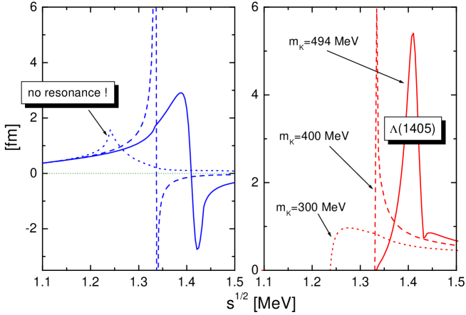
Figure 1: Real (l.h.s.) and imaginary (r.h.s.) part of the isospin zero s-wave $K^{-}$-nucleon scattering amplitude as it follows from the $SU(3)$ Weinberg-Tomozawa interaction term in a coupled channel calculation. We use $f=93$ MeV and identify the subtraction point with the $\Lambda(1116)$ mass.

In Fig. 1 we anticipate our final result for the leading interaction term of the chiral $SU(3)$ Lagrangian density suggested by Tomozawa and Weinberg. If taken as input for the multi-channel Bethe-Salpeter equation, properly furnished with a renormalization scheme leading to a subtraction point close to the baryon octet mass, a rich structure of the scattering amplitude arises. Details for the coupled channel generalization of (79) are presented in the subsequent sections. Fig. 1 shows the s-wave solution of the multi-channel Bethe-Salpeter as a function of the kaon mass. For physical kaon masses the isospin zero scattering amplitude exhibits a resonance structure at energies where one would expect the $\Lambda(1405)$ resonance. We point out that the resonance structure disappears as the kaon mass is decreased. Already at a hypothetical kaon mass of $300$ MeV the $\Lambda(1405)$ resonance is no longer formed. Fig. 1 demonstrates that the chiral $SU(3)$ Lagrangian is necessarily non-perturbative in the strangeness sector. This confirms the findings of [19, 20]. In previous works however the $\Lambda(1405)$ resonance is the result of a fine tuned cutoff parameter which gives rise to a different kaon mass dependence of the scattering amplitude [20]. In our scheme the choice of subtraction point close to the baryon octet mass follows necessarily from the compliance of the expansion scheme with approximate crossing symmetry. Moreover, the identification of the subtraction point with the $\Lambda$-mass in the isospin zero channel protects the hyperon exchange s-channel pole contribution and therefore avoids possible pathologies at subthreshold energies.

We turn to the pion-nucleon sector. The chiral $SU(2)$ Lagrangian has been successfully applied to pion-nucleon scattering in standard chiral perturbation theory [29, 30, 71]. Here the typical expansion parameter $m^{2}_{\pi}/(8\,\pi\,f^{2})\ll 1$ characterizing the unitarization is sufficiently small and one would expect good convergence properties. The application of the chiral $SU(3)$ Lagrangian to pion-nucleon scattering on the other hand is not completely worked out so far. In the SU(3) scheme the $\pi N$ channel couples for example to the $K\Sigma$ channel. Thus the slow convergence of the unitarization in the $K\Sigma$ channel suggests to expand the interaction kernel rather than the scattering amplitude also in the strangeness zero channel. This may improve the convergence properties of the chiral expansion and extend its applicability domain to larger energies. Also, if the same set of parameters are to be used in the pion-nucleon and kaon-nucleon sectors the analogous partial resummation of higher order counter terms included by solving the Bethe-Salpeter equation should be applied. We illustrate such effects for the case of the Weinberg-Tomozawa interaction. With $c^{(\frac{3}{2})}_{\pi N\to\pi N}=-1$ and $c^{(\frac{3}{2})}_{\pi N\to K\Sigma}=-1$ the isospin three half s-wave pion-nucleon scattering lengths $a_{\pi N}^{(\frac{3}{2})}$ receive the typical correction terms

$$4\,\pi\left(1+\frac{m_{\pi}}{m_{N}}\right)a_{\pi N}^{(\frac{3}{2})}=-\frac{m_{\pi}}{2\,f^{2}}\,\Bigg{(}1-\frac{m^{2}_{\pi}}{16\,\pi^{2}\,f^{2}}\left(\pi-\ln\left(\frac{m_{\pi}^{2}}{m_{N}^{2}}\right)\right)$$

$$\qquad\qquad-\frac{(m_{\pi}+m_{K})^{2}}{32\,\pi^{2}\,f^{2}}\Bigg{(}-1-\frac{1}{2}\,\ln\left(\frac{m_{K}^{2}}{m_{\Sigma}^{2}}\right)$$

$$\qquad\qquad+\pi\left(\frac{3\,m_{K}}{4\,m_{N}}-\frac{m_{\Sigma}-m_{N}}{2\,m_{K}}\right)+{\mathcal{O}}\left(Q^{2}\right)\Bigg{)}\Bigg{)}+{\mathcal{O}}\left(m_{\pi}^{2}\right)\;,$$ (81)

where we again considered exclusively the unitary correction terms. Note that the ratio $(m_{\Sigma}-m_{N})/m_{K}$ arises in (81), because we first expand in powers of $m_{\pi}$ and only then expand further with $m_{\Sigma}-m_{N}\sim Q^{2}$ and $m_{K}^{2}\sim Q^{2}$. The correction terms in (81) induced by the kaon-hyperon loop, which is subtracted at the nucleon mass, exemplify the fact that the parameter $f$ is renormalized by the strangeness sector and therefore must not be identified with the chiral limit value of $f$ as derived for the $SU(2)$ chiral Lagrangian. This is evident if one confronts the Weinberg-Tomozawa theorem of the chiral $SU(2)$ symmetry with (81). The expression (81) demonstrates further that this renormalization of $f$ appears poorly convergent in the kaon mass. Note in particular the anomalously large term $\pi\,m_{K}/m_{N}$. Hence it is advantageous to consider the partial resummation induced by a unitary coupled channel treatment of pion-nucleon scattering.

3.4 Partial-wave decomposition of the Bethe-Salpeter equation

The Bethe-Salpeter equation (49) can be solved analytically for quasi-local interaction terms which typically arise in the chiral Lagrangian. The scattering equation is decoupled by introducing relativistic projection operators ${Y}^{(\pm)}_{n}(\bar{q},q;w)$ with good total angular momentum:

$${Y}^{(\pm)}_{n}(\bar{q},q;w)=\frac{1}{2}\,\Bigg{(}\frac{w/}{\sqrt{w^{2}}}\pm 1\Bigg{)}\,\bar{Y}_{n+1}(\bar{q},q;w)$$

$$\;\;\;\;\;\;\;\;\;\;-\frac{1}{2}\,\Bigg{(}\bar{q}/-\frac{w\cdot\bar{q}}{w^{2}}\,w/\Bigg{)}\Bigg{(}\frac{w/}{\sqrt{w^{2}}}\mp 1\Bigg{)}\,\Bigg{(}q/-\frac{w\cdot q}{w^{2}}\,w/\Bigg{)}\bar{Y}_{n}(\bar{q},q;w)\;,$$

$$\bar{Y}_{n}(\bar{q},q;w)=\sum_{k=0}^{[(n-1)/2]}\,\frac{(-)^{k}\,(2\,n-2\,k)!}{2^{n}\,k!\,(n-k)!\,(n-2\,k-1)!}\,Y_{\bar{q}\bar{q}}^{k}\,Y_{\bar{q}q}^{n-2\,k-1}\,Y_{qq}^{k}\;,$$

$$Y_{\bar{q}\bar{q}}=\frac{(w\cdot\bar{q})\,(\bar{q}\cdot w)}{w^{2}}-\bar{q}\cdot\bar{q}\;,\;\;\;Y_{qq}=\frac{(w\cdot q)\,(q\cdot w)}{w^{2}}-q\cdot q\;,$$

$$Y_{\bar{q}q}=\frac{(w\cdot\bar{q})\,(q\cdot w)}{w^{2}}-\bar{q}\cdot q\;.$$ (82)

For the readers convenience we provide the leading order projectors ${Y}_{n}^{(\pm)}$ relevant for the $J={\textstyle{1\over 2}}$ and $J={\textstyle{3\over 2}}$ channels explicitly:

$${Y}_{0}^{(\pm)}(\bar{q},q;w) = \frac{1}{2}\,\left(\frac{w/}{\sqrt{w^{2}}}\pm 1\right)\;,$$

$${Y}_{1}^{(\pm)}(\bar{q},q;w) = \frac{3}{2}\,\left(\frac{w/}{\sqrt{w^{2}}}\pm 1\right)\left(\frac{(\bar{q}\cdot w)\,(w\cdot q)}{w^{2}}-\big{(}\bar{q}\cdot q\big{)}\right)$$ (83)

$$- \frac{1}{2}\,\Bigg{(}\bar{q}/-\frac{w\cdot\bar{q}}{w^{2}}\,w/\Bigg{)}\Bigg{(}\frac{w/}{\sqrt{w^{2}}}\mp 1\Bigg{)}\,\Bigg{(}q/-\frac{w\cdot q}{w^{2}}\,w/\Bigg{)}\;.$$

The objects ${Y}^{(\pm)}_{n}(\bar{q},q;w)$ are constructed to have the following convenient property: Suppose that the interaction kernel $K$ in (49) can be expressed as linear combinations of the ${Y}^{(\pm)}_{n}(\bar{q},q;w)$ with a set of coupling functions $V^{(\pm)}(\sqrt{s}\,,n)$, which may depend on the variable $s$,

$$K(\bar{k},k;w) = \sum_{n=0}^{\infty}\left(V^{(+)}(\sqrt{s};n)\,{Y}^{(+)}_{n}(\bar{q},q;w)+V^{(-)}(\sqrt{s};n)\,{Y}^{(-)}_{n}(\bar{q},q;w)\right)\,,$$ (84)

with $w=p+q$, $k=(p-q)/2$ and $\bar{k}=(\bar{p}-\bar{q})/2$. Then in a given isospin channel the unique solution reads

$$T(\bar{k},k;w)=\sum_{n=0}^{\infty}\left(M^{(+)}(\sqrt{s};n)\,{Y}^{(+)}_{n}(\bar{q},q;w)+M^{(-)}(\sqrt{s};n)\,{Y}^{(-)}_{n}(\bar{q},q;w)\right)\;,$$

$$M^{(\pm)}(\sqrt{s};n)=\frac{V^{(\pm)}(\sqrt{s};n)}{1-V^{(\pm)}(\sqrt{s};n)\,J^{(\pm)}_{\pi N}(\sqrt{s};n)}\;,$$ (85)

with a set of divergent loop functions $J^{(\pm)}_{\pi N}(\sqrt{s};n)$ defined by

$$J^{(\pm)}_{\pi N}(\sqrt{s};n)\,{Y}^{(\pm)}_{n}(\bar{q},q;w) =-i\int\frac{d^{4}l}{(2\pi)^{4}}\,{Y}^{(\pm)}_{n}(\bar{q},l;w)\,S_{N}(w-l)\,$$ (86)

$$\;\;\;\;\;\;\;\;\;\;\;\;\;\;\;\;\;\;\;\;\;\times D_{\pi}(l)\,{Y}^{(\pm)}_{n}(l,q;w)\;.$$

We underline that the definition of the loop functions in (86) is non trivial, because it assumes that $Y_{n}^{(\pm)}\cdot G\cdot Y_{n}^{(\pm)}$ is indeed proportional to $Y_{n}^{(\pm)}$. An explicit derivation of this property, which is in fact closely linked to our renormalization scheme, is given in Appendix C. We recall that the loop functions $J^{(\pm)}_{\pi N}(\sqrt{s};n)$, which are badly divergent, have a finite and well-defined imaginary part

$$\Im\,J^{(\pm)}_{\pi N}(\sqrt{s};n) = \frac{p^{2\,n+1}_{\pi N}}{8\,\pi\,\sqrt{s}}\left(\frac{\sqrt{s}}{2}+\frac{m_{N}^{2}-m_{\pi}^{2}}{2\,\sqrt{s}}\pm m_{N}\right)\;.$$ (87)

We specify how to renormalize the loop functions. In dimensional regularization the loop functions can be written as linear combinations of scalar one loop functions $I_{\pi N}(\sqrt{s}\,)$, $I_{\pi}$, $I_{N}$ and $I^{(n)}$,

$$I^{(n)}=i\,\int\frac{d^{4}l}{(2\pi)^{4}}\,\Big{(}l^{2}\Big{)}^{n}\;,$$ (88)

According to our renormalization procedure we drop $I^{(n)}$, the tadpole contributions $I_{\pi}$, $I_{N}$ and replace $I_{\pi N}(s)$ by $I_{\pi N}(\sqrt{s}\,)-I_{\pi N}(\mu_{S})$. This leads to

$$J^{(\pm)}_{\pi N}(\sqrt{s};n) = p_{\pi N}^{2\,n}(\sqrt{s}\,)\left(\frac{\sqrt{s}}{2}+\frac{m_{N}^{2}-m_{\pi}^{2}}{2\,\sqrt{s}}\pm m_{N}\right)\Delta I_{\pi N}(\sqrt{s}\,)\;,$$

$$\Delta I_{\pi N}(\sqrt{s}\,) = I_{\pi N}(\sqrt{s}\,)-I_{\pi N}(\mu_{S})\;,$$ (89)

with the master loop function $I_{\pi N}(\sqrt{s}\,)$ and $p_{\pi N}(\sqrt{s}\,)$ given in (62). In the center of mass frame $p_{\pi N}$ represents the relative momentum. We emphasize that the loop functions $J^{(\pm)}_{\pi N}(\sqrt{s};n)$ are renormalized in accordance with (76) and (75) where $\mu_{S}=m_{N}$. This leads to tadpole-free loop functions and also to $M^{(\pm)}(m_{N},n)=V^{(\pm)}(m_{N},n)$. The behavior of the loop functions $J^{(\pm)}_{\pi N}(\sqrt{s},n)$ close to threshold

$$\Im\,J^{(+)}_{\pi N}(\sqrt{s},n)\sim p_{\pi N}^{2\,n+1}\;,\qquad\Im\,J^{(-)}_{\pi N}(\sqrt{s},n)\sim p_{\pi N}^{2\,n+3}\,,$$ (90)

already tells the angular momentum, $l$, of a given channel with $l=n$ for the ${}^{\prime}+^{\prime}$ and $l=n+1$ for the ${}^{\prime}-^{\prime}$ channel.

The Bethe-Salpeter equation (85) decouples into reduced scattering amplitudes $M^{(\pm)}(\sqrt{s},n)$ with well-defined angular momentum. In order to unambiguously identify the total angular momentum $J$ we recall the partial-wave decomposition of the on-shell scattering amplitude $T$ [9]. The amplitude $T$ is decomposed into invariant amplitudes $F^{(I)}_{\pm}(s,t)$ carrying good isospin $I$

$$T = \sum_{I}\,\left(\frac{1}{2}\,\Bigg{(}\frac{w/}{\sqrt{w^{2}}}+1\Bigg{)}\,F^{(I)}_{+}(s,t)+\frac{1}{2}\,\Bigg{(}\frac{w/}{\sqrt{w^{2}}}-1\Bigg{)}\,F^{(I)}_{-}(s,t)\right)P_{I}$$ (91)

where $s=(p+q)^{2}=w^{2}$ and $t=(\bar{q}-q)^{2}$ and $P_{I}$ are the isospin projectors introduced in (52). Note that the choice of invariant amplitudes is not unique. Our choice is particularly convenient to make contact with the covariant projection operators (82). For different choices, see [9]. The amplitudes $F_{\pm}(s,t)$ are decomposed into partial-wave amplitudes $f^{(l)}_{J=l\pm\frac{1}{2}}(\sqrt{s}\,)$ [9]

$$F_{+}(s,t) = \frac{8\,\pi\,\sqrt{s}}{E+m_{N}}\,\sum_{n=1}^{\infty}\,\Big{(}f_{J=n+\frac{1}{2}}^{(n-1)}(\sqrt{s}\,)-f_{J=n-\frac{1}{2}}^{(n+1)}(\sqrt{s}\,)\Big{)}\,P^{\prime}_{n}(\cos\theta)\;,$$

$$F_{-}(s,t) = \frac{8\,\pi\,\sqrt{s}}{E-m_{N}}\,\sum_{n=1}^{\infty}\,\Big{(}f_{J=n-\frac{1}{2}}^{(n)}(\sqrt{s}\,)-f_{J=n+\frac{1}{2}}^{(n)}(\sqrt{s}\,)\Big{)}\,P^{\prime}_{n}(\cos\theta)\;,$$

$$P^{\prime}_{n}(\cos\theta) = \sum_{k=0}^{[(n-1)/2]}\,\frac{(-)^{k}\,(2\,n-2\,k)!}{2^{n}\,k!\,(n-k)!\,(n-2\,k-1)!}\,\Big{(}\cos\theta\Big{)}^{n-2\,k-1}\,,$$ (92)

where $[n/2]=(n-1)/2$ for $n$ odd and $[n/2]=n/2$ for $n$ even. $P^{\prime}_{n}(z)$ is the derivative of the Legendre polynomials. In the center of mass frame $E$ represents the nucleon energy and $\theta$ the scattering angle:

$$E=\frac{1}{2}\,\sqrt{s}+\frac{m_{N}^{2}-m_{\pi}^{2}}{2\,\sqrt{s}}\;,\;\;\;t=(\bar{q}-q)^{2}=-2\,p_{\pi N}^{2}\,\Big{(}1-\cos\theta\Big{)}\;.$$ (93)

The unitarity condition formulated for the partial-wave amplitudes $f_{J}^{(l)}$ leads to their representation in terms of the scattering phase shifts $\delta^{(l)}_{J}$

$$p_{\pi N}\,f^{(l)}_{J=l\pm\frac{1}{2}}(\sqrt{s}\,)=\frac{1}{2\,i}\left(e^{2\,i\,\delta^{(l)}_{J=l\pm\frac{1}{2}}(s)}-1\right)=\frac{1}{\cot\delta^{(l)}_{J=l\pm\frac{1}{2}}(s)-i}\;.$$ (94)

One can now match the reduced amplitudes $M^{(\pm)}_{n}(s)$ of (85) and the partial-wave amplitudes $f^{(l)}_{J=l\pm\frac{1}{2}}(s)$

$$f^{(l)}_{J=l\pm\frac{1}{2}}(\sqrt{s}\,) = \frac{p^{2\,J-1}_{\pi N}}{8\,\pi\,\sqrt{s}}\left(\frac{\sqrt{s}}{2}+\frac{m_{N}^{2}-m_{\pi}^{2}}{2\,\sqrt{s}}\pm m_{N}\right)M^{(\pm)}(\sqrt{s},J-{\textstyle{1\over 2}})\;.$$ (95)

It is instructive to consider the basic building block $\bar{Y}_{n}(\bar{q},q;w)$ of the covariant projectors ${Y}_{n}^{(\pm)}(\bar{q},q;w)$ in (82) and observe the formal similarity with $P^{\prime}_{n}(\cos\theta)$ in (92). In fact in the center of mass frame with $w_{cm}=(\sqrt{s},0)$ one finds $p_{\pi N}^{2\,n-2}\,P^{\prime}_{n}(\cos\theta)=Y_{n}(\bar{q},q;w_{cm})$. This observation leads to a straightforward proof of (85) and (86). It is sufficient to prove the orthogonality of the projectors ${Y}_{n}^{(\pm)}(\bar{q},q;w)$ in the center of mass frame, because the projectors are free from kinematical singularities. One readily finds that the imaginary part of the unitary products ${Y}^{(\pm)}_{n}\,G\,{Y}^{(\pm)}_{m}$ vanish unless both projectors are the same. It follows that the unitary product of projectors which are expected to be orthogonal can at most be a real polynomial involving the tadpole functions $I_{\pi},I_{N}$ and $I^{(n)}$. Then our renormalization procedure as described in section 3.2 leads to (85) and (86). We emphasize that our argument relies crucially on the fact that the projectors ${Y}_{n}^{(\pm)}(\bar{q},q;w)$ are free from kinematical singularities in $q$ and $\bar{q}$. This implies in particular that the object $Y_{n}(\bar{q},q;w)$ must not be identified with $p_{\pi N}^{2\,n-2}\,P^{\prime}_{n}(\cos\theta)$ as one may expect naively.

We return to the assumption made in (84) that the interaction kernel $K$ can be decomposed in terms of the projectors $Y_{n}^{(\pm)}$. Of course this is not possible for a general interaction kernel $K$. We point out, however, that the on-shell equivalent interaction kernel $V$ in (54) can be decomposed into the $Y_{n}^{(\pm)}$ if the on-shell irreducible kernel $\bar{K}$ and the on-shell reducible kernels $K_{L,R}$ and $K_{LR}$ of (53) are identified properly. The on-shell irreducible kernel $\bar{K}$ of (53) is defined by decomposing the interaction kernel according to

$$\bar{K}^{(I)}(\bar{q},q;w)=\sum_{n=0}^{\infty}\left(\bar{K}^{(I)}_{+}(\sqrt{s};n)\,{Y}_{n}^{(+)}(\bar{q},q;w)+\bar{K}^{(I)}_{-}(\sqrt{s};n)\,{Y}_{n}^{(-)}(\bar{q},q;w)\right)\;,$$

$$\bar{K}^{(I)}_{\pm}(\sqrt{s};n)=\int_{-1}^{1}\frac{dz}{2}\,\frac{K^{(I)}_{\pm}(s,t)}{\,p^{2\,n}_{\pi N}}\,P_{n}(z)$$

$$\;\;\;\;\;\;\;\;\;\;\;\;\;\;\;\;+\int_{-1}^{1}\frac{dz}{2}\,\left(\frac{1}{2}\,\sqrt{s}+\frac{m_{N}^{2}-m_{\pi}^{2}}{2\,\sqrt{s}}\mp m_{N}\right)^{2}\frac{K^{(I)}_{\mp}(s,t)}{p^{2\,n+2}_{\pi N}}\,P_{n+1}(z)\;,$$ (96)

where $t=-2\,p_{\pi N}^{2}\,(1-x)$ and $K_{\pm}^{(I)}(s,t)$ follows from the decomposition of the interaction kernel $K$:

$$K^{(I)}(\bar{q},q;w)\Big{|}_{\rm{on-shell}}=\frac{1}{2}\,\Bigg{(}\frac{w/}{\sqrt{w^{2}}}+1\Bigg{)}\,K_{+}^{(I)}(s,t)+\frac{1}{2}\,\Bigg{(}\frac{w/}{\sqrt{w^{2}}}-1\Bigg{)}\,K_{-}^{(I)}(s,t)\;.$$ (97)

Then $K-\bar{K}$ is on-shell reducible by construction and therefore can be decomposed into $K_{L},K_{R},K_{LR}$. Note that it does not yet follow that the induced effective interaction $V$ can be decomposed into the $Y_{n}^{(\pm)}$. This may need an iterative procedure in particular when the interaction kernel shows non-local structures induced for example by a $t$-channel meson-exchange. The starting point of the iteration is given with $K_{0}=K$ and $V_{0}=\bar{K}$ as defined via (96). Then $K_{n+1}=V[K_{n}]$, where $V[K_{n}]$ is defined in (55) with respect to $\bar{K}_{n}$ as given in (96). The effective interaction $V$ is then identified with $V=^{\rm\;\;\;\,lim}_{\;n\to\infty}\,\bar{K}_{n}$. In our work we will not encounter this complication, because the effective interaction kernel is treated to leading orders of chiral perturbation theory.

4 $SU(3)$ coupled-channel dynamics

The Bethe-Salpeter equation (49) is readily generalized for a coupled-channel system. The chiral $SU(3)$ Lagrangian with baryon octet and pseudo-scalar meson octet couples the $\bar{K}N$ system to five inelastic channels $\pi\Sigma$, $\pi\Lambda$, $\eta\Lambda$, $\eta\Sigma$ and $K\Xi$ and the $\pi N$ system to the three channels $K\Sigma$, $\eta N$ and $K\Lambda$. The strangeness plus one sector with the $KN$ channel is treated separately in the next section when discussing constraints from crossing symmetry. For simplicity we assume in the following discussion good isospin symmetry. Isospin symmetry breaking effects are considered in Appendix D. In order to establish our convention consider for example the two-body meson-baryon interaction terms in (24). They can be rewritten in the following form

$${\mathcal{L}}(\bar{k},k;w) = \sum_{I=0,\frac{1}{2},1,\frac{3}{2}}\,R^{(I)\,\dagger}(\bar{q},\bar{p})\,\gamma_{0}\,K^{(I)}(\bar{k},k;w)\,R^{(I)}(q,p)\,,\;\;\;\;$$

$$R^{(0)} = \left(\begin{array}[]{c}\textstyle{1\over\sqrt{2}}\,K^{\dagger}\,N\\ \textstyle{1\over\sqrt{3}}\,\vec{\pi}_{c}\;\vec{\Sigma}\\ \eta_{c}\,\Lambda\\ \textstyle{1\over\sqrt{2}}\,K^{t}\,i\,\sigma_{2}\,\Xi\end{array}\right)\;,\;\;\;\vec{R}^{(1)}=\left(\begin{array}[]{c}\textstyle{1\over\sqrt{2}}\,K^{\dagger}\,\vec{\sigma}\,N\\ \textstyle{1\over i\sqrt{2}}\,\vec{\pi}_{c}\,\times\vec{\Sigma}\\ \vec{\pi}_{c}\,\Lambda\\ \eta_{c}\,\vec{\Sigma}\\ \textstyle{1\over\sqrt{2}}\,K^{t}\,i\,\sigma_{2}\,\vec{\sigma}\,\Xi\end{array}\right)\;,$$ (107)

$$R^{(\frac{1}{2})} = \left(\begin{array}[]{c}\textstyle{1\over\sqrt{3}}\,\pi_{c}\cdot\sigma\,N\\ \textstyle{1\over\sqrt{3}}\,\Sigma\cdot\sigma\,K\\ \eta_{c}\,N\\ K\,\Lambda\end{array}\right)\;,\;\;\;\;R^{(\frac{3}{2})}=\left(\begin{array}[]{c}\pi_{c}\cdot S\,N\\ \Sigma\cdot S\,K\end{array}\right)\;,$$ (114)

where $R(q,p)$ in (114) is defined by $R(q,p)=\int d^{4}x\,d^{4}y\,e^{-i\,q\,x-i\,p\,y}\,\Phi(x)\,B(y)$, and $\Phi(x)$ and $B(y)$ denoting the meson and baryon fields respectively. In (114) we decomposed the pion field $\vec{\pi}=\vec{\pi}_{c}+\vec{\pi}_{c}^{\dagger}$ and the eta field $\eta=\eta_{c}+\eta_{c}^{\dagger}$. Also we apply the isospin decomposition of (12). The isospin $1/2$ to $3/2$ transition matrices $S_{i}$ in (114) are normalized by $S^{\dagger}_{i}\,S_{j}=\delta_{ij}-\sigma_{i}\,\sigma_{j}/3$. The Lagrangian density ${\mathcal{L}}(x)$ in coordinate space is related to its momentum space representation through

$$\int d^{4}x\,{\mathcal{L}}(x) = \int\frac{d^{4}k}{(2\,\pi)^{4}}\,\frac{d^{4}\bar{k}}{(2\,\pi)^{4}}\,\frac{d^{4}w}{(2\,\pi)^{4}}\,{\mathcal{L}}(\bar{k},k;w)\;.$$ (115)

The merit of the notation (114) is threefold. Firstly, the phase convention for the isospin states is specified. Secondly, it defines the convention for the interaction kernel $K$ in the Bethe-Salpeter equation. Last it provides also a convenient scheme to read off the isospin decomposition for the interaction kernel $K$ directly from the interaction Lagrangian (see Appendix A). The coupled channel Bethe-Salpeter matrix equation reads

$$T^{(I)}_{ab}(\bar{k},k;w) = K^{(I)}_{ab}(\bar{k},k;w)+\sum_{c,d}\int\!\!\frac{d^{4}l}{(2\pi)^{4}}\,K^{(I)}_{ac}(\bar{k},l;w)\,G^{(I)}_{cd}(l;w)\,T^{(I)}_{db}(l,k;w)\;,$$

$$G^{(I)}_{cd}(l;w) = -i\,D_{\Phi(I,d)}({\textstyle\frac{1}{2}}\,w-l)\,S_{B(I,d)}({\textstyle\frac{1}{2}}\,w+l)\,\delta_{cd}\,,$$ (116)

where $D_{\Phi(I,d)}(q)$ and $S_{B(I,d)}(p)$ denote the meson propagator and baryon propagator respectively for a given channel $d$ with isospin $I$. The matrix structure of the coupled-channel interaction kernel $K_{ab}(\bar{k},k;w)$ is defined via (114) and

$$\Phi(0,a)=(\bar{K},\pi,\eta,K)_{a}\;,\;\;\;\;\;\;\ B(0,a)=(N,\Sigma,\Lambda,\Xi)_{a}\;,$$

$$\Phi(1,a)=(\bar{K},\pi,\pi,\eta,K)_{a}\;,\;\;\ B(1,a)=(N,\Sigma,\Lambda,\Sigma,\Xi)_{a}\;,$$

$$\Phi({\textstyle{1\over 2}},a)=(\pi,K,\eta,K)_{a}\;,\;\;\;\;\;\;\ B({\textstyle{1\over 2}},a)=(N,\Sigma,N,\Lambda)_{a}\;,$$

$$\Phi({\textstyle{3\over 2}},a)=(\pi,K)_{a}\;,\;\;\qquad\quad\;\;B({\textstyle{3\over 2}},a)=(N,\Sigma)_{a}\;.$$ (117)

We proceed and identify the on-shell equivalent coupled channel interaction kernel $V$ of (55). At leading chiral orders it is legitimate to identify $V^{(I)}_{ab}$ with $\bar{K}^{(I)}_{ab}$ of (53), because the loop corrections in (55) are of minimal chiral power $Q^{3}$ (see (9)). To chiral order $Q^{3}$ the interaction kernel receives additional terms from one loop diagrams involving the on-shell reducible interaction kernels $K_{L,R}$ as well as from irreducible one-loop diagrams. In the notation of (53) one finds

$$V=\bar{K}+K_{R}\cdot G\cdot\bar{K}+\bar{K}\,\cdot G\cdot K_{L}+K_{R}\cdot G\cdot K_{L}+{\mathcal{O}}\left(Q^{4}\right)\;.$$ (118)

Typically the $Q^{3}$ terms induced by $K_{L,R}$ in (118) are tadpoles (see e.g. (60,79)). The only non-trivial contribution arise from the on-shell reducible parts of the u-channel baryon octet terms. However, by construction, those contributions have the same form as the irreducible $Q^{3}$ loop-correction terms of $\bar{K}$. In particular they do not show the typical enhancement factor of $2\pi$ associated with the s-channel unitarity cuts. In the large $N_{c}$ limit all loop correction terms to $V$ are necessarily suppressed by $1/N_{c}$. This follows, because any hadronic loop function if visualized in terms of quark-gluon diagrams involves at least one quark-loop, which in turn is $1/N_{c}$ suppressed [23, 24]. Thus it is legitimate to take $V=\bar{K}$ in this work.

We do include those correction terms of suppressed order in the $1/N_{c}$ expansion which are implied by the physical baryon octet and decuplet exchange contributions. Individually the baryon exchange diagrams are of forbidden order $N_{c}$. Only the complete large $N_{c}$ baryon ground state multiplet with $J=({\textstyle{1\over 2}},...,{\textstyle{N_{c}\over 2}})$ leads to an exact cancellation and a scattering amplitude of order $N_{c}^{0}$ [72]. However this cancellation persists only in the limit of degenerate baryon octet $m^{\!\!\!\!{}^{o}}_{[8]}$ and decuplet mass $m^{\!\!\!\!{}^{o}}_{[10]}$. With $m_{\pi}<m^{\!\!\!\!{}^{o}}_{[10]}-m^{\!\!\!\!{}^{o}}_{[8]}$ the cancellation is incomplete and thus leads to an enhanced sensitivity of the scattering amplitude to the physical baryon-exchange contributions. Therefore one should sum the $1/N_{c}$ suppressed contributions of the form $(m^{\!\!\!\!{}^{o}}_{[10]}-m^{\!\!\!\!{}^{o}}_{[8]})^{n}/m_{\pi}^{n}\sim N_{c}^{-n}$. We take this into account by evaluating the baryon-exchange contributions to subleading chiral orders but avoid the expansion in either of $(m^{\!\!\!\!{}^{o}}_{[10]}-m^{\!\!\!\!{}^{o}}_{[8]})/m_{\pi}$ or $m_{\pi}/(m^{\!\!\!\!{}^{o}}_{[10]}-m^{\!\!\!\!{}^{o}}_{[8]})$. We also include the $SU(3)$ symmetry-breaking counter terms of the 3-point meson-baryon vertices and the quasi-local two-body counter terms of chiral order $Q^{3}$ which are leading in the $1/N_{c}$ expansion. Note that the quasi-local two-body counter terms of large chiral order are not necessarily suppressed by $1/N_{c}$ relatively to the terms of low chiral order. This is plausible, because for example a t-channel vector-meson exchange, which has a definite large $N_{c}$ scaling behavior, leads to contributions in all partial waves. Thus quasi-local counter terms with different partial-wave characteristics may have identical large $N_{c}$ scaling behavior even though they carry different chiral powers. Finally we argue that it is justified to perform the partial $1/N_{c}$ resummation of all reducible diagrams implied by solving the Bethe-Salpeter equation (54). In section 3 we observed that reducible diagrams are typically enhanced close to their unitarity threshold. The typical enhancement factor of $2\pi$ per unitarity cut, measured relatively to irreducible diagrams (see (80)), is larger than the number of colors $N_{c}=3$ of our world.

By analogy with (85) the coupled-channel scattering amplitudes $T^{(I)}_{ab}$ are decomposed into their on-shell equivalent partial-wave amplitudes $M^{(I,\pm)}_{ab}$

$$\bar{T}^{(I)}_{ab}(\bar{k},k;w) = \sum_{n=0}^{\infty}\,M^{(I,+)}_{ab}(\sqrt{s};n)\,{Y}_{n}^{(+)}(\bar{q},q;w)$$ (119)

$$+ \sum_{n=0}^{\infty}\,M^{(I,-)}_{ab}(\sqrt{s};n)\,{Y}_{n}^{(-)}(\bar{q},q;w)\;,$$

where $k=\!{\textstyle{1\over 2}}\,w-q$ and $\bar{k}=\!{\textstyle{1\over 2}}\,w-\bar{q}$ and $s=w_{\mu}\,w^{\mu}$. The covariant projectors ${Y}_{n}^{(\pm)}(\bar{q},q;w)$ were defined in (82). Expressions for the differential cross sections given in terms of the partial-wave amplitudes $M_{ab}^{(\pm)}$ can be found in Appendix F. The form of the scattering amplitude (119) follows, because the effective interaction kernel $V^{(I)}_{ab}$ of (55) is decomposed accordingly

$$V^{(I)}_{ab}(\bar{k},k;w) = \sum_{n=0}^{\infty}\,V^{(I,+)}_{ab}(\sqrt{s};n)\,{Y}_{n}^{(+)}(\bar{q},q;w)$$ (120)

$$+ \sum_{n=0}^{\infty}\,V^{(I,-)}_{ab}(\sqrt{s};n)\,{Y}_{n}^{(-)}(\bar{q},q;w)\;.$$

The coupled-channel Bethe-Salpeter equation (116) reduces to a convenient matrix equation for the effective interaction kernel $V^{(I)}_{ab}$ and the invariant amplitudes $M^{(I,\pm)}_{ab}$

$$M^{(I,\pm)}_{ab}(\sqrt{s};n) = V^{(I,\pm)}_{ab}(\sqrt{s};n)$$ (121)

$$+ \sum_{c,d}V^{(I,\pm)}_{ac}(\sqrt{s};n)\,J^{(I,\pm)}_{cd}(\sqrt{s};n)\,M^{(I,\pm)}_{db}(\sqrt{s};n)\;,$$

which is readily solved with:

$$M^{(I,\pm)}_{ab}(\sqrt{s};n) = \Bigg{[}\left(1-V^{(I,\pm)}(\sqrt{s};n)\,J^{(I,\pm)}(\sqrt{s};n)\right)^{-1}V^{(I,\pm)}(\sqrt{s};n)\Bigg{]}_{ab}\,.$$ (122)

It remains to specify the coupled-channel loop matrix function $J^{(I,\pm)}_{ab}\!\!\sim\delta_{ab}$, which is diagonal in the coupled-channel space. We write

$$J^{(I,\pm)}_{aa}(\sqrt{s};n)=\left(\frac{\sqrt{s}}{2}+\frac{m_{B(I,a)}^{2}-m_{\Phi(I,a)}^{2}}{2\,\sqrt{s}}\pm m_{B(I,a)}\right)\Delta I^{(k)}_{\Phi(I,a)\,B(I,a)}(\sqrt{s}\,)$$

$$\qquad\qquad\qquad\!\times\left(\frac{s}{4}-\frac{m_{B(I,a)}^{2}+m_{\Phi(I,a)}^{2}}{2}+\frac{\big{(}m_{B(I,a)}^{2}-m_{\Phi(I,a)}^{2}\big{)}^{2}}{4\,s}\right)^{n}\;,$$

$$\Delta I^{(k)}_{\Phi(I,a)\,B(I,a)}(\sqrt{s}\,)=I_{\Phi(I,a)\,B(I,a)}(\sqrt{s}\,)$$

$$\qquad\qquad\qquad\quad-\sum_{l=0}^{k}\,\frac{1}{l}\left(\frac{\partial}{\partial\,\sqrt{s}}\right)^{l}\,\Bigg{|}_{\sqrt{s}=\mu_{S}}\,I_{\Phi(I,a)\,B(I,a)}(\sqrt{s}\,)\;.$$ (123)

The index $a$ labels a specific channel consisting of a meson-baryon pair of given isospin ($\Phi(I,a)$, $B(I,a)$). In particular $m_{\Phi(I,a)}$ and $m_{B(I,a)}$ denote the empirical isospin averaged meson and baryon octet mass respectively. The scalar master-loop integral, $I_{\Phi(I,a)\,B(I,a)}(\sqrt{s}\,)$, was introduced explicitly in (62) for the pion-nucleon channel. Note that we do not use the expanded form of (63). The subtraction point $\mu_{S}^{(I)}$ is identified with $\mu_{S}^{(0)}\!=\!m_{\Lambda}$ and $\mu_{S}^{(1)}\!=\!m_{\Sigma}$ in the isospin zero and isospin one channel respectively so as to protect the hyperon s-channel pole structures. Similarly we use $\mu_{S}^{(\frac{1}{2})}=\mu_{S}^{(\frac{3}{2})}=m_{N}$ in the pion-nucleon sector. We emphasize that in the p-wave loop functions $J^{(-)}(\sqrt{s},0)$ and $J^{(+)}(\sqrt{s},1)$ we perform a double subtraction of the internal master-loop function with $k=1$ in (123) whenever a large $N_{c}$ baryon ground state manifests itself with a s-channel pole contribution in the associated partial-wave scattering amplitude. In all remaining channels we use $k=0$ in (123). This leads to consistency with the renormalization condition (76), in particular in the large $N_{c}$ limit with $m_{[8]}=m_{[10]}$.

We proceed by identifying the on-shell irreducible interaction kernel $\bar{K}^{(I)}_{ab}$ in (118). The result (96) is generalized to the case of inelastic scattering. This leads to the matrix structure of the interaction kernel $K_{ab}$ defined in (114). In a given partial wave the effective interaction kernel $\bar{K}^{(I,\pm)}_{ab}(\sqrt{s};n)$ reads

$$\bar{K}^{(I)}_{ab}=\sum_{n=0}^{\infty}\left(\bar{K}^{(I,+)}_{ab}(\sqrt{s};n)\,{Y}_{n}^{(+)}(\bar{q},q;w)+\bar{K}^{(I,-)}_{ab}(\sqrt{s};n)\,{Y}_{n}^{(-)}(\bar{q},q;w)\right)\;,$$

$$\bar{K}^{(I,\pm)}_{ab}(\sqrt{s};n)=\int_{-1}^{1}\frac{dz}{2}\,\frac{K^{(I,\pm)}_{ab}(s,t^{(I)}_{ab})}{\big{(}p^{(I)}_{a}\,p^{(I)}_{b}\big{)}^{n}}\,P_{n}(z)$$

$$\;\;\;\;\;\;\;\;\;\;\;+\int_{-1}^{1}\frac{dz}{2}\,\,\Big{(}E^{(I)}_{a}\mp m_{B(I,a)}\Big{)}\,\Big{(}E^{(I)}_{b}\mp m_{B(I,b)}\Big{)}\frac{K^{(I,\mp)}_{ab}(s,t^{(I)}_{ab})}{\big{(}p^{(I)}_{a}\,p^{(I)}_{b}\big{)}^{n+1}}\,P_{n+1}(z)\;,$$ (124)

where $P_{n}(z)$ are the Legendre polynomials and

$$t^{(I)}_{ab}=m_{\Phi(I,a)}^{2}+m_{\Phi(I,b)}^{2}-2\,\omega^{(I)}_{a}\,\omega^{(I)}_{b}+2\,p^{(I)}_{a}\,p^{(I)}_{b}\,z\;,\;\;\;E^{(I)}_{a}=\sqrt{s}-\omega^{(I)}_{a}\;,$$

$$\omega^{(I)}_{a}=\frac{s+m^{2}_{\Phi(I,a)}-m^{2}_{B(I,a)}}{2\,\sqrt{s}}\;,\;\;\;\Big{(}p^{(I)}_{a}\Big{)}^{2}=\Big{(}\omega^{(I)}_{a}\Big{)}^{2}-m_{\Phi(I,a)}^{2}\;.$$ (125)

The construction of the on-shell irreducible interaction kernel requires the identification of the invariant amplitudes $K_{ab}^{(I,\pm)}(s,t)$ in a given channel $ab$:

$$K^{(I)}_{ab}\Big{|}_{\rm{on-sh.}}=\frac{1}{2}\,\Bigg{(}\frac{w/}{\sqrt{w^{2}}}+1\Bigg{)}\,K_{ab}^{(I,+)}(s,t)+\frac{1}{2}\,\Bigg{(}\frac{w/}{\sqrt{w^{2}}}-1\Bigg{)}\,K_{ab}^{(I,-)}(s,t)\;.$$ (126)

Isospin breaking effects are easily incorporated by constructing super matrices $V^{(I^{\prime}I)}$, $J^{(I^{\prime}I)}$ and $T^{(I^{\prime}I)}$ which couple different isospin states. We consider isospin breaking effects induced by isospin off-diagonal loop function $J^{(I^{\prime}I)}$ but impose $V^{(I^{\prime}I)}\sim\delta_{I^{\prime}I}$. For technical details we refer to Appendix D.

We underline that our approach deviates here from the common chiral expansion scheme as implied by the heavy-fermion representation of the chiral Lagrangian. A strict chiral expansion of the unitarity loop function $I_{\Phi(I,a)\,B(I,a)}(\sqrt{s}\,)$ does not reproduce the correct s-channel unitarity cut. One must perform an infinite summation of interaction terms in the heavy-fermion chiral Lagrangian to recover the correct threshold behavior. This is achieved more conveniently by working directly with the manifest relativistic scheme, where it is natural to write down the loop functions in terms of the physical masses. In this work we express results systematically in terms of physical parameters avoiding the use of bare parameters like $m^{\!\!\!\!{}^{o}}_{[8]}$ whenever possible.

4.1 Construction of effective interaction kernel

We collect all terms of the chiral Lagrangian contributing to order $Q^{3}$ to the interaction kernel $K^{(I)}_{ab}(\bar{k},k;w)$ of (116):

$$K^{(I)}(\bar{k},k;w) = K^{(I)}_{WT}(\bar{k},k;w)+K^{(I)}_{s-[8]}(\bar{k},k;w)+K^{(I)}_{u-[8]}(\bar{k},k;w)$$ (127)

$$+ K^{(I)}_{s-[10]}(\bar{k},k;w)+K^{(I)}_{u-[10]}(\bar{k},k;w)+K^{(I)}_{s-[9]}(\bar{k},k;w)$$

$$+ K^{(I)}_{u-[9]}(\bar{k},k;w)+K^{(I)}_{[8][8]}(\bar{k},k;w)+K^{(I)}_{\chi}(\bar{k},k;w)\,.$$

The various contributions to the interaction kernel will be written in a form which facilitates the derivation of $K^{(I,\pm)}_{ab}(s,t)$ in (124). It is then straightforward to derive the on-shell irreducible interaction kernel $V$.

We begin with a discussion of the Weinberg-Tomozawa interaction term $K^{(I)}_{WT}$ in (11). To chiral order $Q^{3}$ it is necessary to consider the effects of the baryon wave-function renormalization factors ${\mathcal{Z}}$ and of the further counter terms introduced in (38). We have

$$\Big{[}\,K^{(I)}_{W\,T\,}(\bar{k},k;w)\Big{]}_{ab} = \Big{[}C_{WT}^{(I)}\Big{]}_{ab}\,\Big{(}1+{\textstyle{1\over 2}}\,\Delta\zeta_{B(I,a)}+{\textstyle{1\over 2}}\,\Delta\zeta_{B(I,b)}\Big{)}\,\frac{\bar{q}/+q/}{4\,f^{2}}\;.$$ (128)

The dimensionless coefficient matrix $C_{WT}^{(I)}$ of the Weinberg-Tomozawa interaction is given in Tab. 2 for the strangeness zero channels and in the Appendix E for the strangeness minus one channels. The constants $\Delta\zeta_{B(c)}$ in (128) receive contributions from the baryon octet wave-function renormalization factors ${\mathcal{Z}}$ and the parameters $\zeta_{0},\zeta_{D}$ and $\zeta_{F}$ of (38):

$$\Delta\zeta=\zeta+{\mathcal{Z}}-1+\cdots\,,$$

$$\zeta_{N}=\big{(}\zeta_{0}+2\,\zeta_{F}\big{)}\,m_{\pi}^{2}+\big{(}2\,\zeta_{0}+2\,\zeta_{D}-2\,\zeta_{F}\big{)}\,m_{K}^{2}\;,$$

$$\zeta_{\Lambda}=\big{(}\zeta_{0}-{\textstyle{2\over 3}}\,\zeta_{D}\big{)}\,m_{\pi}^{2}+\big{(}2\,\zeta_{0}+{\textstyle{8\over 3}}\,\zeta_{D}\big{)}\,m_{K}^{2}\;,$$

$$\zeta_{\Sigma}=\big{(}\zeta_{0}+2\,\zeta_{D}\big{)}\,m_{\pi}^{2}+2\,\zeta_{0}\,m_{K}^{2}\;,$$

$$\zeta_{\Xi}=\big{(}\zeta_{0}-2\,\zeta_{F}\big{)}\,m_{\pi}^{2}+\big{(}2\,\zeta_{0}+2\,\zeta_{D}+2\,\zeta_{F}\big{)}\,m_{K}^{2}\;.$$ (129)

The dots in (129) represent corrections terms of order $Q^{3}$ and further contributions from irreducible one-loop diagrams not considered here. We point out that the coupling constants $\zeta_{0}$, $\zeta_{D}$ and $\zeta_{F}$, which appear to renormalize the strength of the Weinberg-Tomozawa interaction term, also contribute to the baryon wave-function factor ${\mathcal{Z}}$ as is evident from (33). In fact, it will be demonstrated that the explicit and implicit dependence via the wave-function renormalization factors ${\mathcal{Z}}$ cancel identically at leading order. Generalizing (74) we derive the wave-function renormalization constants for the $SU(3)$ baryon octet fields

$${\mathcal{Z}}^{-1}_{B(c)}-1=\zeta_{B(c)}-\frac{1}{4\,f^{2}}\,\sum_{a}\,\xi_{B(I,a)}\,m_{\Phi(I,a)}^{2}\left(G^{(B(c))}_{\Phi(I,a)\,B(I,a)}\right)^{2}\,,$$ (130)

$$\xi_{B(I,a)}=2\,m_{B(c)}\,\frac{\partial\,I_{\Phi(I,a)\,B(I,a)}(\sqrt{s}\,)}{\partial\sqrt{s}}\Bigg{|}_{\sqrt{s}=m_{B(c)}}-\frac{I_{\Phi(I,a)}}{m_{\Phi(I,a)}^{2}}+{\mathcal{O}}\left(Q^{4}\right)\,,$$

where the sum in (130) includes all $SU(3)$ channels as listed in (114). The result (130) is expressed in terms of the dimension less coupling constants $G_{\Phi B}^{(B)}$. For completeness we collect here all required 3-point coupling coefficients:

$$G_{\pi N}^{(N)}=\sqrt{3}\,\Big{(}F+D\Big{)}\;,\quad G_{K\,\Sigma}^{(N)}=-\sqrt{3}\,\Big{(}F-D\Big{)}\;,\quad G_{\eta\,N}^{(N)}={\textstyle{1\over\sqrt{3}}}\,\Big{(}3\,F-D\Big{)}\;,$$

$$G_{K\,\Lambda}^{(N)}=-{\textstyle{1\over\sqrt{3}}}\,\Big{(}3\,F+D\Big{)}\;,\quad G_{\bar{K}N}^{(\Lambda)}=\sqrt{2}\,G_{K\,\Lambda}^{(N)}\;,\quad G_{\pi\Sigma}^{(\Lambda)}=2\,D\;,$$

$$G_{\eta\,\Lambda}^{(\Lambda)}=-{\textstyle{2\over\sqrt{3}}}\,D\;,\quad G_{K\Xi}^{(\Lambda)}=-\sqrt{{\textstyle{2\over 3}}}\,\Big{(}3\,F-D\Big{)}\;,\quad G_{\bar{K}N}^{(\Sigma)}=\sqrt{{\textstyle{2\over 3}}}\,G_{K\Sigma}^{(N)}\;,$$

$$G_{\pi\Sigma}^{(\Sigma)}=-\sqrt{8}\,F\;,\quad G_{\pi\Lambda}^{(\Sigma)}={\textstyle{1\over\sqrt{3}}}\,G_{\pi\Sigma}^{(\Lambda)}\;,\quad G_{\eta\Sigma}^{(\Sigma)}={\textstyle{2\over\sqrt{3}}}\,D\;,$$

$$G_{K\Xi}^{(\Sigma)}=\sqrt{2}\,\Big{(}F+D\Big{)}\;,\quad G_{\bar{K}\Lambda}^{(\Xi)}=-{\textstyle{1\over\sqrt{2}}}\,G_{K\Xi}^{(\Lambda)}\;,\quad G_{\bar{K}\Sigma}^{(\Xi)}=-\sqrt{{\textstyle{3\over 2}}}\,G_{K\Xi}^{(\Sigma)}\;,$$

$$G_{\eta\,\Xi}^{(\Xi)}=-{\textstyle{1\over\sqrt{3}}}\,\Big{(}3\,F+D\Big{)}\;,\quad G_{\pi\,\Xi}^{(\Xi)}=\sqrt{3}\,\Big{(}F-D\Big{)}\;,$$ (131)

at leading chiral order $Q^{0}$. The loop function $I_{\Phi(I,a)\,B(I,a)}(\sqrt{s}\,)$ and the mesonic tadpole term $I_{\Phi(I,a)}$ are the obvious generalizations of $I_{\pi N}(\sqrt{s}\,)$ and $I_{\pi}$ introduced in (62). We emphasize that the contribution $\zeta_{B(c)}$ in (130) is identical to the corresponding contribution in $\Delta\zeta_{B(c)}$. Therefore, if all one-loop effects are dropped, one finds the result

$${\mathcal{Z}}^{-1}=1+\zeta\;,\qquad\Delta\zeta=0+{\mathcal{O}}\left(Q^{3},\frac{1}{N_{c}}\,Q^{2}\right)\;.$$ (132)

Given our renormalization condition (76) that requires the baryon s-channel pole contribution to be represented by the renormalized effective potential $V_{R}$, we conclude that (132) holds in our approximation. Note that the loop correction to ${\mathcal{Z}}$ as given in (130) must be considered as part of the renormalized effective potential $V_{R}$ and consequently should be dropped as they are suppressed by the factor $Q^{3}/N_{c}$. It is evident that the one-loop contribution to the baryon ${\mathcal{Z}}$-factor is naturally moved into $V_{R}$ by that double subtraction with $k=1$ in (123), as explained previously.

	$C_{WT}^{(\frac{1}{2})}$	$C_{N_{[8]}}^{(\frac{1}{2})}$	$C_{\Lambda_{[8]}}^{(\frac{1}{2})}$	$C_{\Sigma_{[8]}}^{(\frac{1}{2})}$	$C_{\Delta_{[10]}}^{(\frac{1}{2})}$	$C_{\Sigma_{[10]}}^{(\frac{1}{2})}$	$\widetilde{C}_{N_{[8]}}^{(\frac{1}{2})}$	$\widetilde{C}_{\Lambda_{[8]}}^{(\frac{1}{2})}$	$\widetilde{C}_{\Sigma_{[8]}}^{(\frac{1}{2})}$	$\widetilde{C}_{\Xi_{[8]}}^{(\frac{1}{2})}$	$\widetilde{C}_{\Delta_{[10]}}^{(\frac{1}{2})}$	$\widetilde{C}_{\Sigma_{[10]}}^{(\frac{1}{2})}$	$\widetilde{C}_{\Xi_{[10]}}^{(\frac{1}{2})}$
$11$	2	1	0	$0$	0	0	-$\frac{1}{3}$	0	0	0	$\frac{4}{3}$	0	0
$12$	$\frac{1}{2}$	1	0	$0$	0	0	0	$\frac{1}{\sqrt{6}}$	-1	0	0	-1	0
$13$	0	1	0	0	0	0	1	0	0	0	0	0	0
$14$	-$\frac{3}{2}$	1	0	$0$	0	0	0	0	$\sqrt{\frac{3}{2}}$	0	0	$\sqrt{\frac{3}{2}}$	0
$22$	2	1	0	$0$	0	0	0	0	0	-$\frac{1}{3}$	0	0	-$\frac{1}{3}$
$23$	-$\frac{3}{2}$	1	0	$0$	0	0	0	0	$\sqrt{\frac{3}{2}}$	0	0	$\sqrt{\frac{3}{2}}$	0
$24$	0	1	0	$0$	0	0	0	0	0	-1	0	0	-1
$33$	0	1	0	0	0	0	1	0	0	0	0	0	0
$34$	-$\frac{3}{2}$	1	0	$0$	0	0	0	$\frac{1}{\sqrt{2}}$	0	0	0	0	0
$44$	0	1	0	$0$	0	0	0	0	0	1	0	0	1
	$C_{WT}^{(\frac{3}{2})}$	$C_{N_{[8]}}^{(\frac{3}{2})}$	$C_{\Lambda_{[8]}}^{(\frac{3}{2})}$	$C_{\Sigma_{[8]}}^{(\frac{3}{2})}$	$C_{\Delta_{[10]}}^{(\frac{3}{2})}$	$C_{\Sigma_{[10]}}^{(\frac{3}{2})}$	$\widetilde{C}_{N_{[8]}}^{(\frac{3}{2})}$	$\widetilde{C}_{\Lambda_{[8]}}^{(\frac{3}{2})}$	$\widetilde{C}_{\Sigma_{[8]}}^{(\frac{3}{2})}$	$\widetilde{C}_{\Xi_{[8]}}^{(\frac{3}{2})}$	$\widetilde{C}_{\Delta_{[10]}}^{(\frac{3}{2})}$	$\widetilde{C}_{\Sigma_{[10]}}^{(\frac{3}{2})}$	$\widetilde{C}_{\Xi_{[10]}}^{(\frac{3}{2})}$
$11$	-1	0	0	0	1	0	$\frac{2}{3}$	0	0	0	$\frac{1}{3}$	0	0
$12$	-1	0	0	0	1	0	0	$\frac{1}{\sqrt{6}}$	$\frac{1}{2}$	0	0	$\frac{1}{2}$	0
$22$	-1	0	0	0	1	0	0	0	0	$\frac{2}{3}$	0	0	$\frac{2}{3}$

Table 2: Weinberg-Tomozawa interaction strengths and baryon exchange coefficients in the strangeness zero channels as defined in (143).

It is instructive to afford a short detour and explore to what extent the parameters $\zeta_{0},\zeta_{D}$ and $\zeta_{F}$ can be dialed to give ${\mathcal{Z}}=1$. In the $SU(3)$ limit with degenerate meson and also degenerate baryon masses one finds a degenerate wave-function renormalization factor ${\mathcal{Z}}$

$${\mathcal{Z}}^{-1}-1=3\,\zeta_{0}+2\,\zeta_{D}-\frac{m_{\pi}^{2}}{(4\pi\,f)^{2}}\left(\frac{5}{3}\,D^{2}+3\,F^{2}\right)\Bigg{(}-4-3\,\ln\left(\frac{m_{\pi}^{2}}{m_{N}^{2}}\right)$$

$$\qquad\qquad\qquad\qquad\qquad\qquad\qquad+3\,\pi\,\frac{m_{\pi}}{m_{N}}+{\mathcal{O}}\left(\frac{m^{2}_{\pi}}{m^{2}_{N}}\right)\Bigg{)}\;,$$ (133)

where we used the minimal chiral subtraction prescription (70). The result (133) agrees identically with the $SU(2)$-result (74) if one formally replaces $g^{2}_{A}$ by $4\,F^{2}+{\textstyle{20\over 9}}\,D^{2}$ in (74). It is clear from (133) that in the $SU(3)$ limit the counter term $3\,\zeta_{0}+2\,\zeta_{D}$ may be dialed such so as to impose ${\mathcal{Z}}=1$. This is no longer possible once the explicit $SU(3)$ symmetry-breaking effects are included. Note however that consistency of the perturbative renormalization procedure suggests that for hypothetical $SU(3)$-degenerate $\xi$-factors in (130) it should be possible to dial $\zeta_{0}$, $\zeta_{D}$ and $\zeta_{F}$ so as to find ${\mathcal{Z}}_{B}=1$ for all baryon octet fields. This is expected, because for example in the $\overline{MS}$-scheme one finds a $SU(3)$-symmetric renormalization scale dependence of $\xi_{B(c)}$ in (130) with $\xi_{B(c)}\sim\ln\mu^{2}$. Indeed in this case the choice

$$\zeta_{0}=\frac{\xi}{4\,f^{2}}\left(\frac{26}{9}\,D^{2}+2\,F^{2}\right)\,,\qquad\zeta_{D}=\frac{\xi}{4\,f^{2}}\left(-D^{2}+3\,F^{2}\right)\,,\quad$$

$$\zeta_{F}=\frac{\xi}{4\,f^{2}}\,\frac{10}{3}\,D\,F\,,$$ (134)

would lead to ${\mathcal{Z}}=1$ for all baryon octet wave functions. We will return to the $SU(3)$ symmetry-breaking effects in the baryon wave-function renormalization factors when discussing the meson-baryon 3-point vertices at subleading orders.

We proceed with the s-channel and u-channel exchange diagrams of the baryon octet. They contribute as follows

$$\Big{[}K^{(I)}_{s-[8]}(\bar{k},k;w)\Big{]}_{ab} = -\sum_{c\,=\,1}^{3}\,\Big{(}\bar{q}/-R^{(I,c)}_{L,ab}\Big{)}\,\frac{\Big{[}C^{(I,c)}_{[8]}\Big{]}_{ab}}{4\,f^{2}\,\big{(}w/+m^{(c)}_{[8]}\big{)}}\,\Big{(}q/-R^{(I,c)}_{R,ab}\Big{)}\;,$$

$$\Big{[}K^{(I)}_{u-[8]}(\bar{k},k;w)\Big{]}_{ab} = \sum_{c\,=\,1}^{4}\,\frac{\Big{[}\widetilde{C}^{(I,c)}_{[8]}\Big{]}_{ab}}{4\,f^{2}}\,\Bigg{(}w/+m^{(c)}_{\,[8]}+\tilde{R}^{(I,c)}_{L,ab}+\tilde{R}^{(I,c)}_{R,ab}$$ (135)

$$- \Big{(}\bar{p}/+m^{(c)}_{\,[8]}+\tilde{R}^{(I,c)}_{L,ab}\Big{)}\,\frac{1}{\widetilde{w}/+m^{(c)}_{\,[8]}}\,\Big{(}p/+m^{(c)}_{\,[8]}+\tilde{R}^{(I,c)}_{R,ab}\Big{)}\Bigg{)}\;,$$

where $\widetilde{w}_{\mu}=p_{\mu}-\bar{q}_{\mu}$. The index $c$ in (135) labels the baryon octet exchange with $c\to(N,\Lambda,\Sigma,\Xi)$. In particular $m^{(c)}_{[8]}$ denotes the physical baryon octet masses and $R^{(I,c)}$ and $\tilde{R}^{(I,c)}$ characterize the ratios of pseudo-vector to pseudo-scalar terms in the meson-baryon vertices. The dimensionless matrices $C_{[8]}$ and $\widetilde{C}_{[8]}$ give the renormalized strengths of the s-channel and u-channel baryon exchanges respectively. They are expressed most conveniently in terms of s-channel $C_{B(c)}$ and u-channel $\tilde{C}_{B(c)}$ coefficient matrices

$$\Big{[}C^{(I,c)}_{[8]}\Big{]}_{ab}=\Big{[}C^{(I)}_{B(c)}\Big{]}_{ab}\,\bar{A}_{\Phi(I,a)B(I,a)}^{(B(c))}\,\bar{A}_{\Phi(I,b)B(I,b)}^{(B(c))}\;,$$

$$\Big{[}\widetilde{C}^{(I,c)}_{[8]}\Big{]}_{ab}=\Big{[}\widetilde{C}^{(I)}_{B(c)}\Big{]}_{ab}\,\bar{A}_{\Phi(I,b)B(I,a)}^{(B(c))}\,\bar{A}_{\Phi(I,a)B(I,b)}^{(B(c))}\;,$$ (136)

and the renormalized three-point coupling constants $\bar{A}$. According to the LSZ-scheme the bare coupling constants, $A$, are related to the renormalized coupling constants, $\bar{A}$, by means of the baryon octet ${\mathcal{Z}}$-factors

$$\bar{A}_{\Phi(I,a)B(I,b)}^{(B(c))}={\mathcal{Z}}^{\frac{1}{2}}_{B(c)}\,A_{\Phi(I,a)B(I,b)}^{(B(c))}\,{\mathcal{Z}}_{B(I,b)}^{\frac{1}{2}}\,.$$ (137)

To leading order $Q^{0}$ the bare coupling constants $A=G(F,D)+{\mathcal{O}}\left(Q^{2}\right)$ are specified in (131). The chiral correction terms to the coupling constants $A$ and $R$ will be discussed in great detail subsequently. In our convention the s-channel coefficients $C_{B(c)}$ are either one or zero and the u-channel coefficients $\tilde{C}_{B(c)}$ represent appropriate Fierz factors resulting from the interchange of initial and final meson states. To illustrate our notation explicitly the coefficients are listed in Tab. 2 for the strangeness zero channels but relegated to Appendix E for the strangeness minus one channel. We stress that the expressions for the s- and u-channel exchange contribution (135) depend on the result (132), because there would otherwise be a factor ${\mathcal{Z}}^{-1}/(1+\zeta)$ in front of both contributions. That would necessarily lead to an asymmetry in the treatment of s- versus u-channel exchange contribution, because the s-channel contribution would be further renormalized by the unitarization. In contrast, we observe in our scheme the proper balance of s- and u-channel exchange contributions in the scattering amplitude, as is required for the realization of the large $N_{c}$ cancellation mechanism [72].

We turn to the $SU(3)$ symmetry-breaking effects in the meson-baryon coupling constants. The 3-point vertices have pseudo-vector and pseudo-scalar components determined by $F_{i}+\delta F_{i}$ and $\bar{F}_{i}$ of (39,40) respectively. We first collect the symmetry-breaking terms in the axial-vector coupling constants $A$ introduced in (137). They are of chiral order $Q^{2}$ but lead to particular $Q^{3}$-correction terms in the scattering amplitudes. One finds

$$A=G(F_{A},D_{A})-\frac{2}{\sqrt{3}}\,(m_{K}^{2}-m_{\pi}^{2})\,\Delta A\;,\quad\tilde{F}_{i}=F_{i}+\delta F_{i}\;,$$

$$\Delta A_{\pi N}^{(N)}=3\,(F_{1}+F_{3})-F_{0}-F_{2}+2\,(\tilde{F}_{4}+\tilde{F}_{5})\;,$$

$$\Delta A_{K\Sigma}^{(N)}={\textstyle{3\over 2}}\,(F_{1}-F_{3})+{\textstyle{1\over 2}}\,(F_{0}-F_{2})-\tilde{F}_{4}+\tilde{F}_{5}\;,$$

$$\Delta A_{\eta\,N}^{(N)}=-F_{1}+3\,F_{3}+{\textstyle{1\over 3}}\,F_{0}-F_{2}+{\textstyle{2\over 3}}\,\tilde{F}_{4}-2\,\tilde{F}_{5}+2\,(\tilde{F}_{6}+{\textstyle{4\over 3}}\,\tilde{F}_{4})\;,$$

$$\Delta A_{K\Lambda}^{(N)}=-{\textstyle{1\over 2}}\,F_{1}-{\textstyle{3\over 2}}\,F_{3}+{\textstyle{1\over 2}}\,F_{0}+{\textstyle{3\over 2}}\,F_{2}+{\textstyle{1\over 3}}\,\tilde{F}_{4}+\tilde{F}_{5}+(F_{7}+{\textstyle{4\over 3}}\,F_{0})\;,$$

$$\Delta A_{\bar{K}N}^{(\Lambda)}=\sqrt{2}\,\Delta A_{K\,\Lambda}^{(N)}\,,\quad$$

$$\Delta A_{\pi\Sigma}^{(\Lambda)}={\textstyle{4\over\sqrt{3}}}\,\tilde{F}_{4}+\sqrt{3}\,(F_{7}+{\textstyle{4\over 3}}\,F_{0})\;,$$

$$\Delta A_{\eta\,\Lambda}^{(\Lambda)}={\textstyle{4\over 3}}\,(F_{0}+\tilde{F}_{4})+2\,(\tilde{F}_{6}+{\textstyle{4\over 3}}\,\tilde{F}_{4})+2\,(F_{7}+{\textstyle{4\over 3}}\,F_{0})\;,$$

$$\Delta A_{K\Xi}^{(\Lambda)}=-{\textstyle{1\over\sqrt{2}}}\,(F_{0}+F_{1})+{\textstyle{3\over\sqrt{2}}}\,(F_{2}+F_{3})-{\textstyle{\sqrt{2}\over 3}}\,(\tilde{F}_{4}-3\,\tilde{F}_{5})-\sqrt{2}\,(F_{7}+{\textstyle{4\over 3}}\,F_{0})\;,$$

$$\Delta A_{\bar{K}N}^{(\Sigma)}=\sqrt{{\textstyle{2\over 3}}}\,\Delta A_{K\Sigma}^{(N)}\;,\quad\Delta A_{\pi\Sigma}^{(\Sigma)}=-4\,\sqrt{{\textstyle{2\over 3}}}\,(F_{2}+\tilde{F}_{5})\;,\quad\Delta A_{\pi\Lambda}^{(\Sigma)}={\textstyle{1\over\sqrt{3}}}\,\Delta A_{\pi\Sigma}^{(\Lambda)}\;,$$

$$\Delta A_{\eta\Sigma}^{(\Sigma)}={\textstyle{4\over 3}}\,(F_{0}-\tilde{F}_{4})+2\,(\tilde{F}_{6}+{\textstyle{4\over 3}}\,\tilde{F}_{4})\;,$$

$$\Delta A_{K\Xi}^{(\Sigma)}=-\sqrt{{\textstyle{3\over 2}}}\,(F_{1}+F_{3})+\sqrt{{\textstyle{1\over 6}}}\,(F_{0}+F_{2})-\sqrt{{\textstyle{2\over 3}}}\,(\tilde{F}_{4}+\tilde{F}_{5})\;,$$

$$\Delta A_{\bar{K}\Lambda}^{(\Xi)}=-{\textstyle{1\over\sqrt{2}}}\,\Delta A_{K\Xi}^{(\Lambda)}\;,\quad\Delta A_{\bar{K}\Sigma}^{(\Xi)}=-\sqrt{{\textstyle{3\over 2}}}\,\Delta A_{K\Xi}^{(\Sigma)}\;,$$

$$\Delta A_{\eta\,\Xi}^{(\Xi)}=F_{1}+3\,F_{3}+{\textstyle{1\over 3}}\,F_{0}+F_{2}+{\textstyle{2\over 3}}\,\tilde{F}_{4}+2\,\tilde{F}_{5}+2\,(\tilde{F}_{6}+{\textstyle{4\over 3}}\,\tilde{F}_{4})\;,$$

$$\Delta A_{\pi\Xi}^{(\Xi)}=F_{0}+3\,F_{1}-F_{2}-3\,F_{3}+2\,(\tilde{F}_{5}-\tilde{F}_{4})\;,$$ (138)

where the renormalized coupling constants $D_{A}$ and $F_{A}$ are given in (43) and $G(F,D)$ in (131). We emphasize that to order $Q^{2}$ the effect of the ${\mathcal{Z}}$-factors in (137) can be accounted for by the following redefinition of the $F_{R},D_{R}$ and $F_{i}$ parameters in (138)

$$F_{R}\to F_{R}+\,\Big{(}2\,m_{K}^{2}+m_{\pi}^{2}\Big{)}\,\Big{(}\zeta_{0}+{\textstyle{2\over 3}}\,\zeta_{D}\Big{)}\,F_{R}\;,\qquad$$

$$D_{R}\to D_{R}+\Big{(}2\,m_{K}^{2}+m_{\pi}^{2}\Big{)}\,\Big{(}\zeta_{0}+{\textstyle{2\over 3}}\,\zeta_{D}\Big{)}\,D_{R}\;,$$

$$F_{0}\to F_{0}+\zeta_{D}\,D_{R}\,,\qquad F_{1}\to F_{1}+\zeta_{F}\,F_{R}\,,\qquad F_{2}\to F_{2}+\zeta_{D}\,F_{R}\,,$$

$$F_{3}\to F_{3}+\zeta_{F}\,F_{R}\,,\qquad\,F_{7}\to F_{7}-{\textstyle{4\over 3}}\,\zeta_{D}\,\,D_{R}\,.$$ (139)

As a consequence the parameters $\zeta_{0}$, $\zeta_{D}$ and $\zeta_{F}$ are redundant in our approximation and can therefore be dropped. It is legitimate to identify the bare coupling constants $A$ with the renormalized coupling constants $\bar{A}$. Note that the same renormalization holds for matrix elements of the axial-vector current.

We recall the large $N_{c}$ result (45). The many parameters $F_{i}$ and $\delta F_{i}$ in (138) are expressed in terms of the seven parameters $c_{i}$ and $\delta c_{i}=\tilde{c}_{i}-c_{i}-\bar{c}_{i}$. For the readers convenience we provide the axial-vector coupling constants, which are most relevant for the pion-nucleon and kaon-nucleon scattering processes, in terms of those large $N_{c}$ parameters

$$A_{\pi N}^{(N)}=\sqrt{3}\,\Big{(}F_{A}+D_{A}\Big{)}+{\textstyle{5\over 3}}\,(c_{1}+\delta c_{1})+c_{2}+\delta c_{2}-a+5\,c_{3}+c_{4}\;,$$

$$A_{\bar{K}N}^{(\Lambda)}=-\sqrt{{\textstyle{2\over 3}}}\,\Big{(}3\,F_{A}+D_{A}\Big{)}+{\textstyle{1\over\sqrt{2}}}\,\Big{(}c_{1}+\delta c_{1}+c_{2}+\delta c_{2}-a-3\,c_{3}+c_{4}\Big{)}\,,$$

$$A_{\bar{K}N}^{(\Sigma)}=-\sqrt{2}\,\Big{(}F_{A}-D_{A}\Big{)}-{\textstyle{1\over\sqrt{6}}}\,\Big{(}{\textstyle{1\over 3}}\,(c_{1}+\delta c_{1})-c_{2}-\delta c_{2}+a-c_{3}+3\,c_{4}\Big{)}\,,$$

$$A_{\pi\Sigma}^{(\Lambda)}=2\,D_{A}+{\textstyle{2\over\sqrt{3}}}\,(c_{1}+\delta c_{1})\;,$$ (140)

where

$$F_{A} = F_{R}-\frac{\beta}{\sqrt{3}}\,\Big{(}{\textstyle{2\over 3}}\,\delta c_{1}+\delta c_{2}-a\Big{)}\,,\qquad\;\;D_{A}=D_{R}-\frac{\beta}{\sqrt{3}}\,\delta c_{1}\,,$$

$$\beta = \frac{m_{K}^{2}+m_{\pi}^{2}/2}{m_{K}^{2}-m_{\pi}^{2}}\,.$$ (141)

The result (140) shows that the axial-vector coupling constants $A_{\pi N}^{(N)}$, $A_{\bar{K}N}^{(\Lambda)}$, $A_{\bar{K}N}^{(\Sigma)}$ and $A_{\pi\Sigma}^{(\Lambda)}$, can be fine tuned with $c_{i}$ in (45) to be off their $SU(3)$ limit values. Moreover, the SU(3) symmetric contribution proportional to $F_{A}$ or $D_{A}$ deviate from their corresponding $F_{R}$ and $D_{R}$ values relevant for matrix elements of the axial-vector current, once non-zero values for $\delta c_{1,2}$ are established. We recall, however, that the values of $F_{R},D_{R}$ and $c_{i}$ are strongly constrained by the weak decay widths of the baryon-octet states (see Tab. 1). Thus the SU(3) symmetry-breaking pattern in the axial-vector current and the one in the meson-baryon axial-vector coupling constants are closely linked.

It is left to specify the pseudo-scalar part, $P$, of the meson-baryon vertices introduced in (40). In (135) their effect was encoded into the $R$ and $\tilde{R}$ parameters with $R,\tilde{R}\sim\bar{F}\sim\bar{c},a$. Applying the large $N_{c}$ result of (46) we obtain

$$R_{L,ab}^{(I,c)}\,A_{\Phi(I,a)\,B(I,a)}^{(B(c))}=\Big{(}m_{B(I,a)}+m_{B(c)}\Big{)}\,P_{\Phi(I,a)\,B(I,a)}^{(B(c))}\;,$$

$$R_{R,ab}^{(I,c)}\,A_{\Phi(I,b)\,B(I,b)}^{(B(c))}=\Big{(}m_{B(I,b)}+m_{B(c)}\Big{)}\,P_{\Phi(I,b)\,B(I,b)}^{(B(c))}\;,$$

$$\tilde{R}_{L,ab}^{(I,c)}\,A_{\Phi(I,b)\,B(I,a)}^{(B(c))}=\Big{(}m_{B(I,a)}+m_{B(c)}\Big{)}\,P_{\Phi(I,b)\,B(I,a)}^{(B(c))}\;,$$

$$\tilde{R}_{R,ab}^{(I,c)}\,A_{\Phi(I,a)\,B(I,b)}^{(B(c))}=\Big{(}m_{B(I,b)}+m_{B(c)}\Big{)}\,P_{\Phi(I,a)\,B(I,b)}^{(B(c))}\;,$$

$$P_{\pi N}^{(N)}=-\Big{(}{\textstyle{5\over 3}}\,\bar{c}_{1}+\bar{c}_{2}+a\Big{)}\,\Big{(}\beta-1\Big{)}\;,\quad P_{K\Sigma}^{(N)}=-\Big{(}{\textstyle{1\over 3}}\,\bar{c}_{1}-\bar{c}_{2}-a\Big{)}\,\Big{(}\beta+{\textstyle{1\over 2}}\Big{)}\;,$$

$$P_{\eta\,N}^{(N)}={\textstyle{7\over 3}}\,\bar{c}_{1}+\bar{c}_{2}+a-\beta\,\Big{(}{\textstyle{1\over 3}}\,\bar{c}_{1}+\bar{c}_{2}+a\Big{)}\;,\qquad$$

$$P_{K\Lambda}^{(N)}=\Big{(}\bar{c}_{1}+\bar{c}_{2}+a\Big{)}\,\Big{(}\beta+{\textstyle{1\over 2}}\Big{)}\;,\qquad P_{\bar{K}N}^{(\Lambda)}=\sqrt{2}\,P_{K\,\Lambda}^{(N)}\,,\qquad$$

$$P_{\pi\Sigma}^{(\Lambda)}=-{\textstyle{2\over\sqrt{3}}}\,\bar{c}_{1}\,\Big{(}\beta-1\Big{)}\;,\quad P_{\eta\,\Lambda}^{(\Lambda)}={\textstyle{2\over 3}}\,\bar{c}_{1}\,\Big{(}5+\beta\Big{)}+2\,\bar{c}_{2}+2\,a\;,\qquad$$

$$P_{K\Xi}^{(\Lambda)}={\textstyle{1\over\sqrt{2}}}\,\Big{(}{\textstyle{1\over 3}}\,\bar{c}_{1}+\bar{c}_{2}+a\Big{)}\,\Big{(}2\,\beta+1\Big{)}\;,\quad P_{\bar{K}N}^{(\Sigma)}=\sqrt{{\textstyle{2\over 3}}}\,P_{K\Sigma}^{(N)}\;,\quad\!\!$$

$$P_{\pi\Sigma}^{(\Sigma)}=\sqrt{{\textstyle{2\over 3}}}\,\Big{(}{\textstyle{4\over 3}}\,\bar{c}_{1}+2\,\bar{c}_{2}+2\,a\Big{)}\,\Big{(}\beta-1\Big{)}\;,\quad P_{\pi\Lambda}^{(\Sigma)}={\textstyle{1\over\sqrt{3}}}\,P_{\pi\Sigma}^{(\Lambda)}\;,$$

$$P_{\eta\Sigma}^{(\Sigma)}=2\,\bar{c}_{1}\,\Big{(}1-{\textstyle{1\over 3}}\,\beta\Big{)}+2\,\bar{c}_{2}+2\,a\;,\qquad$$

$$P_{K\Xi}^{(\Sigma)}=-{\textstyle{1\over\sqrt{6}}}\,\Big{(}{\textstyle{5\over 3}}\,\bar{c}_{1}+\bar{c}_{2}+a\Big{)}\,\Big{(}2\,\beta+1\Big{)}\;,\quad P_{\bar{K}\Lambda}^{(\Xi)}=-{\textstyle{1\over\sqrt{2}}}\,P_{K\Xi}^{(\Lambda)}\;,\quad$$

$$P_{\bar{K}\Sigma}^{(\Xi)}=-\sqrt{{\textstyle{3\over 2}}}\,P_{K\Xi}^{(\Sigma)}\;,\quad P_{\eta\,\Xi}^{(\Xi)}={\textstyle{11\over 3}}\,\bar{c}_{1}+3\,\bar{c}_{2}+3\,a+\beta\,\Big{(}\bar{c}_{1}+\bar{c}_{2}+a\Big{)}\;,\quad\!\!$$

$$P_{\pi\Xi}^{(\Xi)}=\Big{(}{\textstyle{1\over 3}}\,\bar{c}_{1}-\bar{c}_{2}-a\Big{)}\,\Big{(}\beta-1\Big{)}\;,$$ (142)

where $\beta\simeq 1.12$ was introduced in (141). The pseudo-scalar meson-baryon vertices show $SU(3)$ symmetric contribution linear in $\beta\,\bar{c}_{i}$ and symmetry-breaking terms proportional to $\bar{c}_{i}$. We emphasize that, even though the physical meson-baryon coupling constants, $G=A+P$, are the sum of their axial-vector and pseudo-scalar components, it is important to carefully discriminate both types of vertices, because they give rise to quite different behavior for the partial-wave amplitudes off the baryon-octet pole. We expect such effects to be particularly important in the strangeness sectors since there (142) leads to $P^{(\Lambda,\Sigma)}_{KN}\sim m_{K}^{2}$ to be compared to $P_{\pi N}^{(N)}\sim m_{\pi}^{2}$.

We turn to the decuplet exchange terms $K^{(I)}_{s-[10]}$ and $K^{(I)}_{u-[10]}$ in (127). Again we write their respective interaction kernels in a form which facilitates the identification of their on-shell irreducible parts

$$K^{(I)}_{s-[10]}(\bar{k},k;w) = \sum_{c\,=\,1}^{2}\,\frac{C^{(I,c)}_{[10]}}{4\,f^{2}}\,\Bigg{(}\frac{\bar{q}\cdot q}{w/-m_{[10]}^{(c)}}\,-\frac{(\bar{q}\cdot w)\,(w\cdot q)}{(m_{[10]}^{(c)})^{2}\,\big{(}w/-m_{[10]}^{(c)}\big{)}}$$

$$+ \frac{1}{3}\left(\bar{q}/+\frac{\bar{q}\cdot w}{m_{[10]}^{(c)}}\right)\frac{1}{w/+m_{[10]}^{(c)}}\left(q/+\frac{w\cdot q}{m_{[10]}^{(c)}}\right)-\frac{Z_{[10]}}{3\,m_{[10]}^{(c)}}\,\bar{q}/\,q/$$

$$- \frac{Z_{[10]}^{2}}{6\,(m_{[10]}^{(c)})^{2}}\,\bar{q}/\,\Big{(}w/-2\,m_{[10]}^{(c)}\Big{)}\,q/+Z_{[10]}\,\bar{q}/\,\frac{w\cdot q}{3\,(m_{[10]}^{(c)})^{2}}$$

$$+ Z_{[10]}\,\frac{\bar{q}\cdot w}{3\,(m_{[10]}^{(c)})^{2}}\,q/\Bigg{)}\;,$$

$$K^{(I)}_{u-[10]}(\bar{k},k;w) = \sum_{c\,=\,1}^{3}\,\frac{\widetilde{C}^{(I,c)}_{[10]}}{4\,f^{2}}\,\Bigg{(}\frac{\bar{q}\cdot q}{\widetilde{w}/-m_{[10]}^{(c)}}-\frac{(\bar{q}\cdot\widetilde{w})\,(\widetilde{w}\cdot q)}{(m_{[10]}^{(c)})^{2}\,\big{(}\widetilde{w}/-m_{[10]}^{(c)}\big{)}}$$ (143)

$$+ \frac{1}{3}\left(\bar{p}/+m_{[10]}^{(c)}+\frac{q\cdot\widetilde{w}}{m_{[10]}^{(c)}}\right)\frac{1}{\widetilde{w}/+m_{[10]}^{(c)}}\left(p/+m_{[10]}^{(c)}+\frac{\widetilde{w}\cdot\bar{q}}{m_{[10]}^{(c)}}\right)$$

$$- \frac{\widetilde{w}\cdot(q+\bar{q})}{3\,m_{[10]}^{(c)}}-\frac{1}{3}\,\Big{(}w/+m_{[10]}^{(c)}\Big{)}$$

$$+ \frac{Z_{[10]}}{3\,(m_{[10]}^{(c)})^{2}}\,\Big{(}\bar{q}/\,\big{(}\widetilde{w}\cdot q\big{)}+\big{(}\bar{q}\cdot\widetilde{w}\big{)}\,q/+m_{[10]}^{(c)}\,\big{(}\bar{q}/\,q/-2\,(\bar{q}\cdot q)\big{)}\Big{)}$$

$$- \frac{Z_{[10]}^{2}}{6\,(m_{[10]}^{(c)})^{2}}\,\Big{(}\bar{p}/\;\widetilde{w}/\,p/-\widetilde{w}^{2}\,w/+2\,m_{[10]}^{(c)}\,\big{(}\bar{q}/\,q/-2\,q\cdot q\big{)}\Big{)}\Bigg{)}\;.$$

The index $c$ in (143) labels the decuplet exchange with $c\to(\Delta_{[10]},\Sigma_{[10]},\Xi_{[10]})$. The dimensionless matrices $C^{(I,c)}_{[10]}$ and $\widetilde{C}^{(I,c)}_{[10]}$ characterize the strength of the s-channel and u-channel resonance exchanges respectively. Here we apply the notation introduced in (136) also for the resonance-exchange contributions. In particular the decuplet coefficients $C^{(I,c)}_{[10]}$ and $\tilde{C}^{(I,c)}_{[10]}$ are determined by

$$A=G(C_{A})-\frac{2}{\sqrt{3}}\,(m_{K}^{2}-m_{\pi}^{2})\,\Delta A\;,\qquad\tilde{C}_{0}=C_{0}+\delta C_{0}\;,$$

$$\Delta A_{\pi N}^{(\Delta_{[10]})}=\sqrt{2}\,\big{(}-{\textstyle{1\over\sqrt{3}}}\,C_{2}+\sqrt{3}\,C_{3}+{\textstyle{2\over\sqrt{3}}}\,\tilde{C}_{0}\big{)}\;,\quad$$

$$\Delta A_{K\,\Sigma}^{(\Delta_{[10]})}=-\sqrt{2}\,\big{(}{\textstyle{2\over\sqrt{3}}}\,C_{2}-{\textstyle{1\over\sqrt{3}}}\,\tilde{C}_{0}+\sqrt{3}\,C_{1}\big{)}\;,\quad$$

$$\Delta A_{\bar{K}N}^{(\Sigma_{[10]})}=\sqrt{{\textstyle{2\over 3}}}\,\big{(}-{\textstyle{1\over\sqrt{3}}}\,C_{2}+\sqrt{3}\,C_{3}-{\textstyle{1\over\sqrt{3}}}\,\tilde{C}_{0}-\sqrt{3}\,C_{1}\big{)}-\sqrt{2}\,C_{4}\;,\quad$$

$$\Delta A_{\pi\Sigma}^{(\Sigma_{[10]})}=-\sqrt{{\textstyle{2\over 3}}}\,\big{(}{\textstyle{2\over\sqrt{3}}}\,C_{2}+{\textstyle{2\over\sqrt{3}}}\,\tilde{C}_{0}\big{)}-2\,\sqrt{2}\,C_{4}\;,\qquad$$

$$\Delta A_{\pi\Lambda}^{(\Sigma_{[10]})}={\textstyle{2\over\sqrt{3}}}\,(C_{2}-\tilde{C}_{0})\;,\qquad\Delta A_{\eta\Sigma}^{(\Sigma_{[10]})}={\textstyle{2\over\sqrt{3}}}\,C_{2}-{\textstyle{2\over\sqrt{3}}}\,\tilde{C}_{0}\;,\quad$$

$$\Delta A_{K\Xi}^{(\Sigma_{[10]})}=-\sqrt{{\textstyle{2\over 3}}}\,\big{(}-{\textstyle{1\over\sqrt{3}}}\,C_{2}-\sqrt{3}\,C_{3}-{\textstyle{1\over\sqrt{3}}}\,\tilde{C}_{0}+\sqrt{3}\,C_{1}\big{)}+\sqrt{2}\,C_{4}\;,$$

$$\Delta A_{\bar{K}\Lambda}^{(\Xi_{[10]})}=-{\textstyle{1\over\sqrt{3}}}\,\tilde{C}_{0}-\sqrt{3}\,C_{1}-{\textstyle{1\over\sqrt{3}}}\,(3\,C_{4}+2\,C_{2})\;,\quad$$

$$\Delta A_{\bar{K}\,\Sigma}^{(\Xi_{[10]})}={\textstyle{2\over\sqrt{3}}}\,C_{2}-{\textstyle{1\over\sqrt{3}}}\,\tilde{C}_{0}-\sqrt{3}\,C_{1}+\sqrt{3}\,C_{4}\;,\quad$$

$$\Delta A_{\eta\,\Xi}^{(\Xi_{[10]})}={\textstyle{1\over\sqrt{3}}}\,C_{2}+\sqrt{3}\,C_{3}+{\textstyle{2\over\sqrt{3}}}\,\tilde{C}_{0}+\sqrt{3}\,C_{4}\;,\quad$$

$$\Delta A_{\pi\,\Xi}^{(\Xi_{[10]})}={\textstyle{1\over\sqrt{3}}}\,C_{2}+\sqrt{3}\,C_{3}-{\textstyle{2\over\sqrt{3}}}\,\tilde{C}_{0}-\sqrt{3}\,C_{4}\;,$$ (144)

where the $SU(3)$ symmetric contributions $G(C)$ are

$$G_{\pi N}^{(\Delta_{[10]})}=\sqrt{2}\,C\;,\quad G_{K\,\Sigma}^{(\Delta_{[10]})}=-\sqrt{2}\,C\;,\quad G_{\bar{K}N}^{(\Sigma_{[10]})}=\sqrt{{\textstyle{2\over 3}}}\,C\;,$$

$$G_{\pi\Sigma}^{(\Sigma_{[10]})}=-\sqrt{{\textstyle{2\over 3}}}\,C\;,\quad G_{\pi\Lambda}^{(\Sigma_{[10]})}=-C\;,\quad G_{\eta\Sigma}^{(\Sigma_{[10]})}=C\;,\quad G_{K\Xi}^{(\Sigma_{[10]})}=-\sqrt{{\textstyle{2\over 3}}}\,C\;,$$

$$G_{\bar{K}\Lambda}^{(\Xi_{[10]})}=C\;,\quad G_{\bar{K}\,\Sigma}^{(\Xi_{[10]})}=C\;,\quad G_{\eta\,\Xi}^{(\Xi_{[10]})}=-C\;,\quad G_{\pi\,\Xi}^{(\Xi_{[10]})}=-C\;.$$ (145)

We recall that at leading order in the $1/N_{c}$ expansion the five symmetry-breaking parameters $C_{i}$ introduced in (39) are all given in terms of the $c_{i}$ parameters (45). The parameter $\delta C_{0}\sim\tilde{c}_{1}-c_{1}$ and also implicitly $\tilde{C}_{R}$ (see (43)) probe the $\tilde{c}_{1}$ parameter introduced in (44). We emphasize that all $c_{i}$ parameters but $c_{5}$ are determined to a large extent by the decay widths of the baryon octet states and also $\tilde{c}_{1}$ is constrained strongly by the $SU(3)$ symmetry-breaking pattern of the meson-baryon-octet coupling constants (44).

The baryon octet resonance contributions $K^{(I)}_{s-[9]}$ and $K^{(I)}_{u-[9]}$ require special attention, because the way how to incorporate systematically these resonances in a chiral SU(3) scheme is not clear. We present first the s-channel and u-channel contributions as they follow from (11) at tree-level

$$K^{(I)}_{s-[9]}(\bar{k},k;w) = \sum_{c\,=\,0}^{4}\,\frac{C^{(I,c)}_{[9]}}{4\,f^{2}}\,\Bigg{(}-\frac{\bar{q}\cdot q}{w/+m_{[9]}^{(c)}}\,+\frac{(\bar{q}\cdot w)\,(w\cdot q)}{(m_{[9]}^{(c)})^{2}\,\big{(}w/+m_{[9]}^{(c)}\big{)}}$$

$$- \frac{1}{3}\left(\bar{q}/-\frac{\bar{q}\cdot w}{m_{[9]}^{(c)}}\right)\frac{1}{w/-m_{[9]}^{(c)}}\left(q/-\frac{w\cdot q}{m_{[10]}^{(c)}}\right)\Bigg{)}\;,$$

$$K^{(I)}_{u-[9]}(\bar{k},k;w) = \sum_{c\,=\,0}^{4}\,\frac{\widetilde{C}^{(I,c)}_{[9]}}{4\,f^{2}}\,\Bigg{(}-\frac{\bar{q}\cdot q}{\widetilde{w}/+m_{[9]}^{(c)}}+\frac{(\bar{q}\cdot\widetilde{w})\,(\widetilde{w}\cdot q)}{(m_{[9]}^{(c)})^{2}\,\big{(}\widetilde{w}/+m_{[9]}^{(c)}\big{)}}$$ (146)

$$- \frac{1}{3}\left(\bar{p}/-m_{[9]}^{(c)}-\frac{q\cdot\widetilde{w}}{m_{[9]}^{(c)}}\right)\frac{1}{\widetilde{w}/-m_{[9]}^{(c)}}\left(p/-m_{[9]}^{(c)}-\frac{\widetilde{w}\cdot\bar{q}}{m_{[9]}^{(c)}}\right)$$

$$- \frac{\widetilde{w}\cdot(q+\bar{q})}{3\,m_{[9]}^{(c)}}+\frac{1}{3}\,\Big{(}w/-m_{[9]}^{(c)}\Big{)}\Bigg{)}$$

$$- \frac{Z_{[9]}}{3\,(m_{[9]}^{(c)})^{2}}\,\Big{(}\bar{q}/\,\big{(}\widetilde{w}\cdot q\big{)}+\big{(}\bar{q}\cdot\widetilde{w}\big{)}\,q/-m_{[9]}^{(c)}\,\big{(}\bar{q}/\,q/-2\,(\bar{q}\cdot q)\big{)}\Big{)}$$

$$+ \frac{(Z_{[9]})^{2}}{6\,(m_{[9]}^{(c)})^{2}}\,\Big{(}\bar{p}/\;\widetilde{w}/\,p/-\widetilde{w}^{2}\,w/-2\,m_{[9]}^{(c)}\,\big{(}\bar{q}/\,q/-2\,q\cdot q\big{)}\Big{)}\Bigg{)}$$

where the index $c\to(\Lambda(1520),N(1520),\Lambda(1690),\Sigma(1680),\Xi(1820))$ extends over the nonet resonance states. The coefficient matrices $C^{(I,c)}_{[9]}$ and $\widetilde{C}^{(I,c)}_{[9]}$ are constructed by analogy with those of the octet and decuplet contributions (see (131,136)). In particular one has $C_{B^{*}(c)}^{(I)}=C_{B(c)}^{(I)}$ and $\tilde{C}_{B^{*}(c)}^{(I)}=\tilde{C}_{B(c)}^{(I)}$. The coupling constants $A^{(B^{*})}_{\Phi B}=G^{(B)}_{\Phi B}(F_{[9]},D_{[9]})$ are given in terms of the $F_{[9]}$ and $D_{[9]}$ parameters introduced in (11) for all contributions except those for the $\Lambda(1520)$ and $\Lambda(1690)$ resonances

$$G_{\bar{K}N}^{(\Lambda(1520))}=\sqrt{{\textstyle{2\over 3}}}\,\Big{(}3\,F_{[9]}+D_{[9]}\Big{)}\,\sin\vartheta+\sqrt{3}\,C_{[9]}\,\cos\vartheta\;,\quad$$

$$G_{\pi\Sigma}^{(\Lambda(1520))}=-2\,D_{[9]}\,\sin\vartheta+{\textstyle{3\over\sqrt{2}}}\,C_{[9]}\,\cos\vartheta\;,\quad$$

$$G_{\eta\,\Lambda}^{(\Lambda(1520))}={\textstyle{2\over\sqrt{3}}}\,D_{[9]}\,\sin\vartheta+\sqrt{{\textstyle{3\over 2}}}\,C_{[9]}\,\cos\vartheta\;,\quad$$

$$G_{K\Xi}^{(\Lambda(1520))}=\sqrt{{\textstyle{2\over 3}}}\,\Big{(}3\,F_{[9]}-D_{[9]}\Big{)}\,\sin\vartheta-\sqrt{3}\,C_{[9]}\,\cos\vartheta\;$$ (147)

and

$$G_{\bar{K}N}^{(\Lambda(1690))}=-\sqrt{{\textstyle{2\over 3}}}\,\Big{(}3\,F_{[9]}+D_{[9]}\Big{)}\,\cos\vartheta+\sqrt{3}\,C_{[9]}\,\sin\vartheta\;,\quad$$

$$G_{\pi\Sigma}^{(\Lambda(1690))}=2\,D_{[9]}\,\cos\vartheta+{\textstyle{3\over\sqrt{2}}}\,C_{[9]}\,\sin\vartheta\;,\quad$$

$$G_{\eta\,\Lambda}^{(\Lambda(1690))}=-{\textstyle{2\over\sqrt{3}}}\,D_{[9]}\,\cos\vartheta+\sqrt{{\textstyle{3\over 2}}}\,C_{[9]}\,\sin\vartheta\;,\quad$$

$$G_{K\Xi}^{(\Lambda(1690))}=-\sqrt{{\textstyle{2\over 3}}}\,\Big{(}3\,F_{[9]}-D_{[9]}\Big{)}\,\cos\vartheta-\sqrt{3}\,C_{[9]}\,\sin\vartheta\;.$$ (148)

The baryon octet field $B^{*}_{\mu}$ asks for special considerations in a chiral SU(3) scheme as there is no straightforward systematic approximation strategy. Given that the baryon octet and decuplet states are degenerate in the large $N_{c}$ limit, it is natural to impose $m_{[10]}-m_{[8]}\sim Q$. In contrast with that there is no fundamental reason to insist on $m_{N(1520)}-m_{N}\sim Q$, for example. But, only with $m_{[9]}-m_{[8]}\sim Q$ is it feasible to establish consistent power counting rules needed for the systematic evaluation of the chiral Lagrangian. Note that the presence of the baryon octet resonance states in the large $N_{c}$ limit of QCD is far from abvious. Our opinion differs here from the one expressed in [73, 74] where the d-wave baryon octet resonance states are considered as part of an excited large $N_{c}$ ${\bf 70}$-plet. Recall that reducible diagrams summed by the Bethe-Salpeter equation are typically enhanced by a factor of $2\pi$ relatively to irreducible diagrams. We conclude that there are a priori two possibilities: the baryon resonances are a consequence of important coupled-channel dynamics or they are already present in the interaction kernel. An expansion in $2\pi/N_{c}$, in our world with $N_{c}=3$, does not appear useful. The fact that baryon resonances exhibit large hadronic decay widths may be taken as an indication that the coupled-channel dynamics is the driving mechanism for the creation of baryon resonances. Related arguments have been put forward in [75, 76]. Indeed, for instance the $N(1520)$ resonance, was successfully described in terms of coupled channel dynamics, including the vector-meson nucleon channels as an important ingredient [77], but without assuming a preformed resonance structure in the interaction kernel. The successful description of the $\Lambda(1405)$ resonance in our scheme (see Fig. 1) supports the above arguments. For a recent discussion of the competing picture in which the $\Lambda(1405)$ resonance is considered as a quark-model state we refer to [78].

The description of resonances has a subtle consequence for the treatment of the u-channel baryon resonance exchange contribution. If a resonance is formed primarily by the coupled channel dynamics one should not include an explicit bare u-channel resonance contribution in the interaction kernel. The then necessarily strong energy dependence of the resonance self-energy would invalidate the use of (146), because for physical energies $\sqrt{s}>m_{N}+m_{\pi}$ the resonance self-energy is probed far off the resonance pole. Our discussion has non-trivial implications for the chiral SU(3) dynamics. Naively one may object that the effect of the u-channel baryon resonance exchange contribution in (146) can be absorbed to good accuracy into chiral two-body interaction terms in any case. However, while this is true in a chiral $SU(2)$ scheme, this is no longer possible in a chiral $SU(3)$ approach. This follows because chiral symmetry selects a specific subset of all possible $SU(3)$-symmetric two-body interaction terms at given chiral order. In particular one finds that the effect of the $Z_{[9]}$ parameter in (146) can not be absorbed into the chiral two-body parameters $g^{(S)},g^{(V)}$ or $g^{(T)}$ of (24). For that reason we discriminate two possible scenarios. In scenario I we conjecture that the baryon octet resonance states are primarily generated by the coupled channel dynamics of the vector-meson baryon-octet channels. Therefore in this scenario the u-channel resonance exchange contribution of (146) is neglected and only its s-channel contribution is included as a reminiscence of the neglected vector meson channels. Note that this is analogous to the treatment of the $\Lambda(1405)$ resonance, which is generated dynamically in the chiral $SU(3)$ scheme (see Fig. 1). Here a s-channel pole term is generated by the coupled channel dynamics but the associated u-channel term is effectively left out as a much suppressed contribution. In scenario II we explicitly include the s- and the u-channel resonance exchange contributions as given in (146), thereby assuming that the resonance was preformed already in the large $N_{c}$ limit of QCD and only slightly affected by the coupled channel dynamics. Our detailed analyses of the data set clearly favor scenario I. The inclusion of the u-channel resonance exchange contributions appears to destroy the subtle balance of chiral s-wave range terms and makes it impossible to obtain a reasonable fit to the data set. Thus all results presented in this work will be based on scenario I. Note that in that scenario the background parameter $Z_{[9]}$ drops out completely (see (152)).

	$C_{\pi,0}^{(\frac{1}{2})}$	$C_{\pi,D}^{(\frac{1}{2})}$	$C_{\pi,F}^{(\frac{1}{2})}$	$C_{K,0}^{(\frac{1}{2})}$	${C}_{K,D}^{(\frac{1}{2})}$	${C}_{K,F}^{(\frac{1}{2})}$	${C}_{0}^{(\frac{1}{2})}$	${C}_{1}^{(\frac{1}{2})}$	${C}_{D}^{(\frac{1}{2})}$	${C}_{F}^{(\frac{1}{2})}$	$\bar{C}_{1}^{(\frac{1}{2})}$	$\bar{C}_{D}^{(\frac{1}{2})}$	$\bar{C}_{F}^{(\frac{1}{2})}$
$11$	-4	-2	-2	0	0	0	2	0	1	1	0	2	2
$12$	0	$\frac{1}{2}$	-$\frac{1}{2}$	0	$\frac{1}{2}$	-$\frac{1}{2}$	0	1	-$\frac{1}{2}$	$\frac{1}{2}$	-1	-$\frac{1}{2}$	$\frac{1}{2}$
$13$	0	-2	-2	0	0	0	0	0	1	1	0	0	0
$14$	0	$\frac{1}{2}$	$\frac{3}{2}$	0	$\frac{1}{2}$	$\frac{3}{2}$	0	0	-$\frac{1}{2}$	-$\frac{3}{2}$	0	-$\frac{1}{2}$	-$\frac{3}{2}$
$22$	0	0	0	-4	-2	4	2	0	1	-2	0	-1	2
$23$	0	-$\frac{3}{2}$	$\frac{3}{2}$	0	$\frac{5}{2}$	-$\frac{5}{2}$	0	0	-$\frac{1}{2}$	$\frac{1}{2}$	0	$\frac{3}{2}$	-$\frac{3}{2}$
$24$	0	0	0	0	-2	0	0	0	1	0	0	-1	0
$33$	$\frac{4}{3}$	2	-$\frac{10}{3}$	-$\frac{16}{3}$	-$\frac{16}{3}$	$\frac{16}{3}$	2	0	$\frac{5}{3}$	-1	0	0	0
$34$	0	$\frac{1}{2}$	$\frac{3}{2}$	0	-$\frac{5}{6}$	-$\frac{5}{2}$	0	1	$\frac{1}{6}$	$\frac{1}{2}$	-1	-$\frac{1}{2}$	-$\frac{3}{2}$
$44$	0	0	0	-4	-$\frac{10}{3}$	0	2	0	$\frac{5}{3}$	0	0	1	0
	$C_{\pi,0}^{(\frac{3}{2})}$	$C_{\pi,D}^{(\frac{3}{2})}$	$C_{\pi,F}^{(\frac{3}{2})}$	$C_{K,0}^{(\frac{3}{2})}$	${C}_{K,D}^{(\frac{3}{2})}$	${C}_{K,F}^{(\frac{3}{2})}$	${C}_{0}^{(\frac{3}{2})}$	${C}_{1}^{(\frac{3}{2})}$	${C}_{D}^{(\frac{3}{2})}$	${C}_{F}^{(\frac{3}{2})}$	$\bar{C}_{1}^{(\frac{3}{2})}$	$\bar{C}_{D}^{(\frac{3}{2})}$	$\bar{C}_{F}^{(\frac{3}{2})}$
$11$	-4	-2	-2	0	0	0	2	0	1	1	0	-1	-1
$12$	0	-1	1	0	-1	1	0	1	1	-1	-1	1	-1
$22$	0	0	0	-4	-2	-2	2	0	1	1	0	-1	-1

Table 3: Coefficients of quasi-local interaction terms in the strangeness zero channels as defined in (149).

We turn to the quasi-local two-body interaction terms $K_{[8][8]}^{(I)}$ and $K_{\chi}^{(I)}$ in (127). It is convenient to represent the strength of an interaction term in a given channel $(I,a)\to(I,b)$ by means of the dimensionless coupling coefficients $\big{[}C^{(I)}_{..}\big{]}_{ab}$. The $SU(3)$ structure of the interaction terms ${\mathcal{L}}^{(S)}$ and ${\mathcal{L}}^{(V)}$ in (24) are characterized by the coefficients $C^{(I)}_{0}$, $C^{(I)}_{1}$, $C^{(I)}_{D}$, $C^{(I)}_{F}$ and ${\mathcal{L}}^{(T)}$ by $\bar{C}^{(I)}_{1}$, $\bar{C}^{(I)}_{D}$ and $\bar{C}^{(I)}_{F}$. Similarly the interaction terms (33) which break chiral symmetry explicitly are written in terms of the coefficients $C^{(I)}_{\pi,0}$, $C^{(I)}_{\pi,D}$, $C^{(I)}_{\pi,F}$ and $C^{(I)}_{K,0}$, $C^{(I)}_{K,D}$, $C^{(I)}_{K,F}$. We have

$$K^{(I)}_{[8][8]}(\bar{k},k;w) = \frac{\bar{q}\cdot q}{4f^{2}}\,\Big{(}g^{(S)}_{0}\,C^{(I)}_{0}+g^{(S)}_{1}\,C^{(I)}_{1}+g^{(S)}_{D}\,C^{(I)}_{D}+g^{(S)}_{F}\,C^{(I)}_{F}\Big{)}$$

$$+ \frac{1}{16f^{2}}\,\Big{(}q/\,\big{(}p+\bar{p}\big{)}\cdot\bar{q}+\bar{q}/\,\big{(}p+\bar{p}\big{)}\cdot q\Big{)}\,\Big{(}g^{(V)}_{0}\,C^{(I)}_{0}+g^{(V)}_{1}\,C^{(I)}_{1}\Big{)}$$

$$+ \frac{1}{16f^{2}}\,\Big{(}q/\,\big{(}p+\bar{p}\big{)}\cdot\bar{q}+\bar{q}/\,\big{(}p+\bar{p}\big{)}\cdot q\Big{)}\,\Big{(}g^{(V)}_{D}\,C^{(I)}_{D}+g^{(V)}_{F}\,C^{(I)}_{F}\Big{)}$$

$$+ \frac{i}{4f^{2}}\,\Big{(}\bar{q}^{\mu}\,\sigma_{\mu\nu}\,q^{\nu}\Big{)}\,\Big{(}g^{(T)}_{1}\,\bar{C}^{(I)}_{1}+g^{(T)}_{D}\,\bar{C}^{(I)}_{D}+g^{(T)}_{F}\,\bar{C}^{(I)}_{F}\Big{)}\;,$$

$$K^{(I)}_{\chi}(\bar{k},k;w) = \frac{b_{0}}{f^{2}}\,\Big{(}m_{\pi}^{2}\,C^{(I)}_{\pi,0}+m_{K}^{2}\,C^{(I)}_{K,0}\Big{)}+\frac{b_{D}}{f^{2}}\,\Big{(}m_{\pi}^{2}\,C^{(I)}_{\pi,D}+m_{K}^{2}\,C^{(I)}_{K,D}\Big{)}$$ (149)

$$+ \frac{b_{F}}{f^{2}}\,\Big{(}m_{\pi}^{2}\,C^{(I)}_{\pi,F}+m_{K}^{2}\,C^{(I)}_{K,F}\Big{)}\;,$$

where the coefficients $C^{(I)}_{..,ab}$ are listed in Tab. 3 for the strangeness zero channel and shown in Appendix E for the strangeness minus one channel. A complete listing of the $Q^{3}$ quasi-local two-body interaction terms can be found in Appendix B.

4.2 Chiral expansion and covariance

We proceed and detail the chiral expansion strategy for the interaction kernel in which we wish to keep covariance manifestly. Here it is instructive to rewrite first the meson energy $\omega^{(I)}_{a}$ and the baryon energy $E_{a}^{(I)}$ in (124)

$$\omega^{(I)}_{a}(\sqrt{s})=\sqrt{s}-m^{(I)}_{B(I,a)}-\frac{\phi^{(I)}_{a}(\sqrt{s})}{2\,\sqrt{s}}\,,\;\;\;E_{a}^{(I)}(\sqrt{s})=m_{B(I,a)}+\frac{\phi^{(I)}_{a}(\sqrt{s})}{2\,\sqrt{s}}\;,$$

$$\phi^{(I)}_{a}(\sqrt{s})=\Big{(}\sqrt{s}-m_{B(I,a)}\Big{)}^{2}-m_{\Phi(I,a)}^{2}\,,$$ (150)

in terms of the approximate phase-space factor $\phi^{(I)}_{a}(\sqrt{s}\,)$. We assign $\sqrt{s}\sim Q^{0}$ and $\phi^{(I)}_{a}/\sqrt{s}\sim Q^{2}$. This implies a unique decomposition of the meson energy $\omega^{(I)}_{a}$ in the leading term $\sqrt{s}-m_{B(I,a)}\sim Q$ and the subleading term $-\phi_{a}^{(I)}/(2\sqrt{s})\sim Q^{2}$. We stress that our assignment leads to $m_{B(I,a)}$ as the leading chiral moment of the baryon energy $E_{a}^{(I)}$. We differ here from the conventional heavy-baryon formalism which assigns the chiral power $Q$ to the full meson energy $\omega_{a}^{(I)}$. Consistency with (150), in particular with $E_{a}^{(I)}=\sqrt{s}-\omega_{a}^{(I)}$, then results in either a leading chiral moment of the baryon energy $E_{a}^{(I)}$ not equal to the baryon mass or an assignment $\sqrt{s}\;\sim/\;Q^{0}$.

The implications of our relativistic power counting assignment are first exemplified for the case of the quasi-local two-body interaction terms. We derive the effective interaction kernel relevant for the s- and p-wave channels

$$V^{(I,+)}_{[8][8]}(\sqrt{s};0) = \frac{1}{4f^{2}}\,\Big{(}g^{(S)}_{0}+\sqrt{s}\,g_{0}^{(V)}\Big{)}\,\Big{(}\sqrt{s}-M^{(I)}\Big{)}\,C_{0}^{(I)}\,\Big{(}\sqrt{s}-M^{(I)}\Big{)}$$

$$+ \frac{1}{4f^{2}}\,\Big{(}g^{(S)}_{1}+\sqrt{s}\,g_{1}^{(V)}\Big{)}\,\Big{(}\sqrt{s}-M^{(I)}\Big{)}\,C_{1}^{(I)}\,\Big{(}\sqrt{s}-M^{(I)}\Big{)}$$

$$+ \frac{1}{4f^{2}}\,\Big{(}g^{(S)}_{D}+\sqrt{s}\,g_{D}^{(V)}\Big{)}\,\Big{(}\sqrt{s}-M^{(I)}\Big{)}\,C_{D}^{(I)}\,\Big{(}\sqrt{s}-M^{(I)}\Big{)}$$

$$+ \frac{1}{4f^{2}}\,\Big{(}g^{(S)}_{F}+\sqrt{s}\,g_{F}^{(V)}\Big{)}\,\Big{(}\sqrt{s}-M^{(I)}\Big{)}\,C_{F}^{(I)}\,\Big{(}\sqrt{s}-M^{(I)}\Big{)}$$

$$+ {\mathcal{O}}\left(Q^{3}\right)\;,$$

$$V^{(I,-)}_{[8][8]}(\sqrt{s};0) = -\frac{1}{3f^{2}}\,M^{(I)}\,\Big{(}g^{(S)}_{0}\,C_{0}^{(I)}+g^{(S)}_{1}\,C_{1}^{(I)}\Big{)}\,M^{(I)}$$

$$- \frac{1}{3f^{2}}\,M^{(I)}\,\Big{(}g^{(S)}_{D}\,C_{D}^{(I)}+g^{(S)}_{F}\,C_{F}^{(I)}\Big{)}\,M^{(I)}$$

$$+ \frac{1}{4f^{2}}\left(\sqrt{s}+M^{(I)}\right)\Big{(}g^{(T)}_{1}\,\bar{C}_{1}^{(I)}+g^{(T)}_{D}\,\bar{C}_{D}^{(I)}\Big{)}\left(\sqrt{s}+M^{(I)}\right)$$

$$+ \frac{1}{4f^{2}}\left(\sqrt{s}+M^{(I)}\right)g^{(T)}_{F}\,\bar{C}_{F}^{(I)}\left(\sqrt{s}+M^{(I)}\right)$$

$$- \frac{1}{3f^{2}}\,M^{(I)}\,\Big{(}g^{(T)}_{1}\,\bar{C}_{1}^{(I)}+g^{(T)}_{D}\,\bar{C}_{D}^{(I)}+g^{(T)}_{F}\,\bar{C}_{F}^{(I)}\Big{)}\,M^{(I)}+{\mathcal{O}}\left(Q\right)\;,$$

$$V^{(I,+)}_{[8][8]}(\sqrt{s};1) = -\frac{1}{12f^{2}}\,\Big{(}g^{(S)}_{0}\,C_{0}^{(I)}+g^{(S)}_{1}\,C_{1}^{(I)}+g^{(S)}_{D}\,C_{D}^{(I)}+g^{(S)}_{F}\,C_{F}^{(I)}\Big{)}$$

$$- \frac{1}{12f^{2}}\,\Big{(}g^{(T)}_{1}\,\bar{C}_{1}^{(I)}+g^{(T)}_{D}\,\bar{C}_{D}^{(I)}+g^{(T)}_{T}\,\bar{C}_{F}^{(I)}\Big{)}+{\mathcal{O}}\left(Q\right)\;.$$

$$V^{(I,+)}_{\chi}(\sqrt{s},0) = \frac{b_{0}}{f^{2}}\,\Big{(}m_{\pi}^{2}\,C^{(I)}_{\pi,0}+m_{K}^{2}\,C^{(I)}_{K,0}\Big{)}+\frac{b_{D}}{f^{2}}\,\Big{(}m_{\pi}^{2}\,C^{(I)}_{\pi,D}+m_{K}^{2}\,C^{(I)}_{K,D}\Big{)}$$ (151)

$$+ \frac{b_{F}}{f^{2}}\,\Big{(}m_{\pi}^{2}\,C^{(I)}_{\pi,F}+m_{K}^{2}\,C^{(I)}_{K,F}\Big{)}+{\mathcal{O}}\left(Q^{3}\right)\;,$$

where we introduced the diagonal baryon mass matrix $M^{(I)}_{ab}=\delta_{ab}\,m_{B(I,a)}$. Our notation in (151) implies a matrix multiplication of the mass matrix $M^{(I)}$ by the coefficient matrices $C^{(I)}$ in the ’$ab$’ channel-space. Recall that the d-wave interaction kernel $V^{(I,-)}_{[8][8]}(\sqrt{s},1)$ does not receive any contribution from quasi-local counter terms to chiral order $Q^{3}$. Similarly the chiral symmetry-breaking interaction kernel $V_{\chi}$ can only contribute to s-wave scattering to this order. We point out that the result (151) is uniquely determined by expanding the meson energy according to (150). In particular we keep in $V^{(I,+)}_{\Phi B}(\sqrt{s},0)$ the $\sqrt{s}$ factor in front of $g^{(V)}$. We refrain from any further expansion in $\sqrt{s}-\Lambda$ with some scale $\Lambda\simeq m_{N}$. The relativistic chiral Lagrangian supplied with (150) leads to well defined kinematical factors included in (151). These kinematical factors, which are natural ingredients of the relativistic chiral Lagrangian, can be generated also in the heavy-baryon formalism by a proper regrouping of interaction terms. The $Q^{3}$-terms induced by the interaction kernel (149) are shown in Appendix B as part of a complete collection of relevant $Q^{3}$-terms.

Next we consider the Weinberg-Tomozawa term and the baryon octet and decuplet s-channel pole contributions

$$V^{(I,\pm)}_{WT}(\sqrt{s};0) = \frac{1}{2\,f^{2}}\,\left(\sqrt{s}\,C^{(I)}_{WT}\mp\frac{1}{2}\,\Big{[}M^{(I)}\,,C^{(I)}_{WT}\Big{]}_{+}\right)\;,$$

$$V^{(I,\pm)}_{s-[8]}(\sqrt{s};0) = -\sum_{c=1}^{3}\,\Big{(}\sqrt{s}\mp M^{(I,c)}_{5}\Big{)}\,\frac{C^{(I,c)}_{[8]}}{4\,f^{2}\,\big{(}\sqrt{s}\pm m^{(c)}_{[8]}\big{)}}\,\Big{(}\sqrt{s}\mp M^{(I,c)}_{5}\Big{)}\,,$$

$$V^{(I,+)}_{s-[10]}(\sqrt{s};0) = -\frac{2}{3}\,\sum_{c=1}^{2}\,\frac{\sqrt{s}+m^{(c)}_{[10]}}{(m^{(c)}_{[10]})^{2}}\,\Big{(}\sqrt{s}-M^{(I)}\Big{)}\,\frac{C^{(I,c)}_{[10]}}{4\,f^{2}}\,\Big{(}\sqrt{s}-M^{(I)}\Big{)}$$

$$+ \sum_{c=1}^{2}\,Z_{[10]}\,\frac{2\,\sqrt{s}-m^{(c)}_{[10]}}{3\,(m^{(c)}_{[10]})^{2}}\,\Big{(}\sqrt{s}-M^{(I)}\Big{)}\,\frac{C^{(I,c)}_{[10]}}{4\,f^{2}}\,\Big{(}\sqrt{s}-M^{(I)}\Big{)}$$

$$+ \sum_{c=1}^{2}\,Z_{[10]}^{2}\,\frac{2\,m^{(c)}_{[10]}-\sqrt{s}}{6\,(m^{(c)}_{[10]})^{2}}\,\Big{(}\sqrt{s}-M^{(I)}\Big{)}\,\frac{C^{(I,c)}_{[10]}}{4\,f^{2}}\,\Big{(}\sqrt{s}-M^{(I)}\Big{)}$$

$$+ {\mathcal{O}}\left(Q^{3}\right)\;,$$

$$V^{(I,-)}_{s-[10]}(\sqrt{s};0) = \sum_{c=1}^{2}\,\frac{Z_{[10]}}{3\,m^{(c)}_{[10]}}\,\Big{(}\sqrt{s}+M^{(I)}\Big{)}\,\frac{C^{(I,c)}_{[10]}}{4\,f^{2}}\,\Big{(}\sqrt{s}+M^{(I)}\Big{)}$$

$$- \sum_{c=1}^{2}\,Z_{[10]}^{2}\,\frac{\sqrt{s}+2\,m^{(c)}_{[10]}}{6\,(m^{(c)}_{[10]})^{2}}\,\Big{(}\sqrt{s}+M^{(I)}\Big{)}\,\frac{C^{(I,c)}_{[10]}}{4\,f^{2}}\,\Big{(}\sqrt{s}+M^{(I)}\Big{)}$$

$$+ {\mathcal{O}}\left(Q\right)\;,$$

$$V^{(I,+)}_{s-[10]}(\sqrt{s};+1) = -\frac{1}{3}\,\sum_{c=1}^{2}\,\frac{C^{(I,c)}_{[10]}}{4\,f^{2}\,(\sqrt{s}-m^{(c)}_{[10]})}+{\mathcal{O}}\left(Q\right)\;,$$

$$V^{(I,-)}_{s-[9]}(\sqrt{s};-1) = -\frac{1}{3}\,\sum_{c=1}^{2}\,\frac{C^{(I,c)}_{[9]}}{4\,f^{2}\,(\sqrt{s}-m^{(c)}_{[9]})}+{\mathcal{O}}\left(Q^{0}\right)\;$$ (152)

where we suppressed terms of order $Q^{3}$ and introduced:

$$\Big{[}M^{(I,c)}_{5}\Big{]}_{ab}=\delta_{ab}\,\Big{(}m_{B(I,a)}+R^{(I,c)}_{L,aa}\Big{)}\;.$$ (153)

The Weinberg-Tomozawa interaction term $V_{WT}$ contributes to the s-wave and p-wave interaction kernels with $J=\frac{1}{2}$ to chiral order $Q$ and $Q^{2}$ respectively but not in the $J=\frac{3}{2}$ channels. Similarly the baryon octet s-channel exchange $V_{s-[8]}$ contributes only in the $J=\frac{1}{2}$ channels and the baryon decuplet s-channel exchange $V_{s-[10]}$ to all considered channels but the d-wave channel. The $Q^{3}$-terms not shown in (152) are given in Appendix B. In (152) we expanded also the baryon-nonet resonance contribution applying in particular the questionable formal rule $\sqrt{s}-m_{[9]}\sim Q$. To order $Q^{3}$ one then finds that only the d-wave interaction kernels are affected. In fact, the vanishing of all contributions except the one in the d-wave channel does not depend on the assumption $\sqrt{s}-m_{[9]}\sim Q$. It merely reflects the phase space properties of the resonance field. We observe that our strategy preserves the correct pole contribution in $V^{(I,-)}_{s-[9]}(\sqrt{s};-1)$ but discards smooth background terms in all partial-wave interaction kernels. That is consistent with our discussion of section 4.1 which implies that those background terms are not controlled in any case. We emphasize that we keep the physical mass matrix $M^{(I)}$ rather than the chiral $SU(3)$ limit value in the interaction kernel. Since the mass matrix follows from the on-shell reduction of the interaction kernel it necessarily involves the physical mass matrix $M^{(I)}$. Similarly we keep $M^{(I)}_{5}$ unexpanded since only that leads to the proper meson-baryon coupling strengths. This procedure is analogous to keeping the physical masses in the unitarity loop functions $J_{MB}(w)$ in (86).

We proceed with the baryon octet and baryon decuplet u-channel contributions. After performing their proper angular average as implied by the partial-wave projection in (124) their contributions to the scattering kernels are written in terms of matrix valued functions ${h}^{(I)}_{n\pm}(\sqrt{s},m),{q}^{(I)}_{n\pm}(\sqrt{s},m)$ and ${p}^{(I)}_{n\pm}(\sqrt{s},m)$ as

$$\Big{[}V^{(I,\pm)}_{u-[8]}(\sqrt{s};n)\Big{]}_{ab} = \sum_{c=1}^{4}\,\frac{1}{4\,f^{2}}\,\Big{[}\widetilde{C}^{(I,c)}_{[8]}\Big{]}_{ab}\,\Big{[}{h}^{(I)}_{n\pm}(\sqrt{s},m^{(c)}_{[8]})\Big{]}_{ab}\;,$$

$$\Big{[}V^{(I,\pm)}_{u-[10]}(\sqrt{s};n)\Big{]}_{ab} = \sum_{c=1}^{3}\,\frac{1}{4\,f^{2}}\,\Big{[}\widetilde{C}^{(I,c)}_{[10]}\Big{]}_{ab}\,\Big{[}{p}^{(I)}_{n\pm}(\sqrt{s},m_{[10]}^{(c)})\Big{]}_{ab}\;,$$

$$\Big{[}V^{(I,\pm)}_{u-[9]}(\sqrt{s};n)\Big{]}_{ab} = \sum_{c=1}^{4}\,\frac{1}{4\,f^{2}}\,\Big{[}\widetilde{C}^{(I,c)}_{[9]}\Big{]}_{ab}\,\Big{[}{q}^{(I)}_{n\pm}(\sqrt{s},m^{(c)}_{[9]})\Big{]}_{ab}\;.$$ (154)

The functions ${h}^{(I)}_{n\pm}(\sqrt{s},m),{q}^{(I)}_{n\pm}(\sqrt{s},m)$ and ${p}^{(I)}_{n\pm}(\sqrt{s},m)$ can be expanded in chiral powers once we assign formal powers to the typical building blocks

$$\mu_{\pm,ab}^{(I)}({s},m)=m_{B(I,a)}+m_{B(I,b)}-\sqrt{s}\pm m\;.$$ (155)

We count $\mu_{-}\sim Q$ and $\mu_{+}\sim Q^{0}$ but refrain from any further expansion. Then the baryon octet functions ${h}^{(I)}_{n\pm}(\sqrt{s},m)$ to order $Q^{3}$ read

$$\Big{[}{h}_{0+}^{(I)}(\sqrt{s},m)\Big{]}_{ab}=\sqrt{s}+m+\tilde{R}^{(I,c)}_{L,ab}+\tilde{R}^{(I,c)}_{R,ab}-\frac{m+M_{ab}^{(L)}}{\mu_{+,ab}^{(I)}({s},m)}\,\Bigg{(}\sqrt{s}+$$

$$\qquad\qquad+\frac{\phi^{(I)}_{a}({s})\,(\sqrt{s}-m_{B(I,b)})}{\mu_{+,ab}^{(I)}({s},m)\,\mu_{-,ab}^{(I)}({s},m)}+\frac{(\sqrt{s}-m_{B(I,a)})\,\phi^{(I)}_{b}({s})}{\mu_{+,ab}^{(I)}({s},m)\,\mu_{-,ab}^{(I)}({s},m)}$$

$$\qquad\qquad+\frac{1}{3}\,\frac{\phi^{(I)}_{a}({s})\,(4\,\sqrt{s}-\mu_{+,ab}^{(I)}({s},m))\,\phi^{(I)}_{b}({s})}{\big{(}\mu_{+,ab}^{(I)}({s},m)\big{)}^{2}\,\big{(}\mu_{-,ab}^{(I)}({s},m)\big{)}^{2}}\Bigg{)}\,\frac{m+M_{ab}^{(R)}}{\sqrt{s}}+{\mathcal{O}}\left(Q^{3}\right)\,,$$

$$\Big{[}{h}_{0-}^{(I)}(\sqrt{s},m)\Big{]}_{ab}=\frac{m+M_{ab}^{(L)}}{\mu_{-,ab}^{(I)}({s},m)}\,\Bigg{(}2\,\sqrt{s}+\mu_{-,ab}^{(I)}({s},m)$$

$$\qquad\qquad-\frac{8}{3}\,\frac{m_{B(I,a)}\,m_{B(I,b)}}{\mu_{+,ab}^{(I)}({s},m)}\Bigg{)}\,\frac{m+M_{ab}^{(R)}}{\mu_{+,ab}^{(I)}({s},m)}+{\mathcal{O}}\left(Q\right)\,,$$

$$\Big{[}{h}_{1+}^{(I)}(\sqrt{s},m)\Big{]}_{ab}=-\frac{2}{3}\,\frac{(m+M_{ab}^{(L)})\,(m+M_{ab}^{(R)})}{\mu_{-,ab}^{(I)}({s},m)\,\big{(}\mu_{+,ab}^{(I)}({s},m)\big{)}^{2}}+{\mathcal{O}}\left(Q\right)$$

$$\Big{[}{h}_{1-}^{(I)}(\sqrt{s},m)\Big{]}_{ab}=-\frac{32}{15}\,\frac{(m+M_{ab}^{(L)})\,m_{B(I,a)}\,m_{B(I,b)}\,(m+M_{ab}^{(R)})}{\big{(}\mu_{-,ab}^{(I)}({s},m)\big{)}^{2}\,\big{(}\mu_{+,ab}^{(I)}({s},m)\big{)}^{3}}$$

$$\qquad\qquad+\frac{4}{3}\,\frac{(m+M_{ab}^{(L)})\,\sqrt{s}\,(m+M_{ab}^{(R)})}{\big{(}\mu_{-,ab}^{(I)}({s},m)\big{)}^{2}\,\big{(}\mu_{+,ab}^{(I)}({s},m)\big{)}^{2}}+{\mathcal{O}}\left(Q^{-1}\right)\;,$$ (156)

where we introduced $M_{ab}^{(L)}=m_{B(I,a)}+\tilde{R}^{(I,c)}_{L,ab}$ and $M_{ab}^{(R)}=m_{B(I,b)}+\tilde{R}^{(I,c)}_{R,ab}$. The terms of order $Q^{3}$ can be found in Appendix G where we present also the analogous expressions for the decuplet and baryon-octet resonance exchanges. We emphasize two important points related to the expansion in (156). First, it leads to a separable interaction kernel. Thus the induced Bethe-Salpeter equation is solved conveniently by the covariant projector method of section 3.4. Secondly, such an expansion is only meaningful in conjunction with the renormalization procedure outlined in section 3.2. The expansion leads necessarily to further divergencies which require careful attention.

We close this section with a more detailed discussion of the u-channel exchange. Its non-local nature necessarily leads to singularities in the partial-wave scattering amplitudes at subthreshold energies. For instance, the expressions (156) as they stand turn useless at energies $\sqrt{s}\simeq m_{B(I,a)}+m_{B(I,b)}-m$ due to unphysical multiple poles at $\mu_{-}=0$. One needs to address this problem, because the subthreshold amplitudes are an important input for the many-body treatment of the nuclear meson dynamics. We stress that a singular behavior in the vicinity of $\mu_{-}\sim 0$ is a rather general property of any u-channel exchange contribution. It is not an artifact induced by the chiral expansion. The partial-wave decomposition of a u-channel exchange contribution represents the pole term only for sufficiently large or small $\sqrt{s}$. To be explicit we consider the u-channel nucleon pole term contribution of elastic $\pi N$ scattering

$$\sum_{n=0}^{\infty}\,\int_{-1}^{1}\frac{dx}{2}\,\frac{P_{n}(x)}{\mu_{\pi N}^{(+)}\,\mu_{\pi N}^{(-)}-2\,\phi_{\pi N}\,x+{\mathcal{O}}\left(Q^{3}\right)}\;,$$ (157)

where $\mu^{(\pm)}_{\pi N}=2\,m_{N}-\sqrt{s}\pm m_{N}$. Upon inspecting the branch points induced by the angular average one concludes that the partial wave decomposition (157) is valid only if $\sqrt{s}>\Lambda_{+}$ or $\sqrt{s}<\Lambda_{-}$ with $\Lambda_{\pm}=m_{N}\pm m^{2}_{\pi}/m_{N}+{\mathcal{O}}(Q^{3})$. For any value in between, $\Lambda_{-}<\sqrt{s}<\Lambda_{+}$, the partial-wave decomposition is not converging. We therefore adopt the following prescription for the $u$-channel contributions. The unphysical pole terms in (156) are systematically replaced by

$$m\,\Lambda^{(\pm)}_{ab}(m)=m\,(m_{B(I,a)}+m_{B(I,b)})-m^{2}$$

$$\qquad\qquad\pm\left(\Big{(}(m-m_{B(I,b)})^{2}-m_{\Phi(I,a)}^{2}\Big{)}\,\Big{(}(m-m_{B(I,a)})^{2}-m_{\Phi(I,b)}^{2}\Big{)}\right)^{1/2}\;,$$

$$\left(\mu^{-1}_{-,ab}(\sqrt{s},m)\right)^{n}\rightarrow\left(\mu^{-1}_{-,ab}(\Lambda_{ab}^{(-)},m)\right)^{n}\,\frac{\sqrt{s}-\Lambda_{ab}^{(+)}}{\Lambda_{ab}^{(-)}-\Lambda_{ab}^{(+)}}$$

$$\qquad\qquad\qquad\quad\;+\,\left(\mu^{-1}_{-,ab}(\Lambda_{ab}^{(+)},m)\right)^{n}\,\frac{\sqrt{s}-\Lambda_{ab}^{(-)}}{\Lambda_{ab}^{(+)}-\Lambda_{ab}^{(-)}}\;,$$ (158)

for $\Lambda_{ab}^{(-)}<\sqrt{s}<\Lambda_{ab}^{(+)}$ but kept unchanged for $\sqrt{s}>\Lambda^{(+)}_{ab}$ or $\sqrt{s}<\Lambda^{(-)}_{ab}$ in a given channel (a,b). The prescription (158) properly generalizes the $SU(2)$ sector result $\Lambda_{\pm}\simeq m_{N}\pm m^{2}_{\pi}/m_{N}$ to the $SU(3)$ sector. We underline that (158) leads to regular expressions for $h_{\pm n}(\sqrt{s},m)$ but leaves the u-channel pole contributions unchanged above threshold. The reader may ask why we impose such a prescription at all. Outside the convergence radius of the partial-wave expansion the amplitudes do not make much sense in any case. Our prescription is nevertheless required due to a coupled-channel effect. To be specific, consider for example elastic kaon-nucleon scattering in the strangeness minus one channel. Since there are no u-channel exchange contributions in this channel the physical partial-wave amplitudes do not show any induced singularity structures. For instance in the $\pi\Sigma\to\pi\Sigma$ channel, on the other hand, the u-channel hyperon exchange does contribute and therefore leads through the coupling of the $\bar{K}N$ and $\pi\Sigma$ channels to a singularity also in the $\bar{K}N$ amplitude. Such induced singularities are an immediate consequence of the approximate treatment of the u-channel exchange contribution and must be absent in an exact treatment. As a measure for the quality of our prescription we propose the accuracy to which the resulting subthreshold forward kaon-nucleon scattering amplitudes satisfies a dispersion integral. We return to this issue in the result section.

4.3 $SU(3)$ dynamics in the $S=1$ channels

We turn to the $K^{+}$-nucleon scattering process which is related to the $K^{-}$-nucleon scattering process by crossing symmetry. The scattering amplitudes $T^{(I)}_{KN\rightarrow KN}$ follow from the $K^{-}$-nucleon scattering amplitudes $T^{(I)}_{\bar{K}N\rightarrow\bar{K}N}$ via the transformation

$$T^{(0)}_{KN\rightarrow KN}(\bar{q},q;w)=-\frac{1}{2}\,T^{(0)}_{\bar{K}N\rightarrow\bar{K}N}(-q,-\bar{q};w-\bar{q}-q)$$

$$\quad\quad\quad\quad\quad+\frac{3}{2}\,T^{(1)}_{\bar{K}N\rightarrow\bar{K}N}(-q,-\bar{q};w-\bar{q}-q)\;,$$

$$T^{(1)}_{KN\rightarrow KN}(\bar{q},q;w)=+\frac{1}{2}\,T^{(0)}_{\bar{K}N\rightarrow\bar{K}N}(-q,-\bar{q};w-\bar{q}-q)$$

$$\quad\quad\quad\quad\quad+\frac{1}{2}\,T^{(1)}_{\bar{K}N\rightarrow\bar{K}N}(-q,-\bar{q};w-\bar{q}-q)\;.$$ (159)

It is instructive to work out the implication of crossing symmetry for the kaon-nucleon scattering amplitudes in more detail. We decompose the on-shell scattering amplitudes into their partial-wave amplitudes:

$$T^{(I)}_{KN\rightarrow KN}(\bar{q},q;w)=\frac{1}{2}\,\Bigg{(}\frac{w/}{\sqrt{w^{2}}}+1\Bigg{)}\,F^{(I,+)}_{KN}(s,t)+\frac{1}{2}\,\Bigg{(}\frac{w/}{\sqrt{w^{2}}}-1\Bigg{)}\,F^{(I,-)}_{KN}(s,t)$$

$$\quad\quad\quad=\sum_{n=0}^{\infty}\,\Big{(}M^{(I,+)}_{KN}(\sqrt{s};n)\,{Y}^{(+)}_{n}(\bar{q},q;w)+M^{(I,-)}_{KN}(\sqrt{s};n)\,{Y}^{(-)}_{n}(\bar{q},q;w)\Big{)}\;,$$

$$T^{(I)}_{\bar{K}N\rightarrow\bar{K}N}(\bar{q},q;w)=\frac{1}{2}\,\Bigg{(}\frac{w/}{\sqrt{w^{2}}}+1\Bigg{)}\,F^{(I,+)}_{\bar{K}N}(s,t)+\frac{1}{2}\,\Bigg{(}\frac{w/}{\sqrt{w^{2}}}-1\Bigg{)}\,F^{(I,-)}_{\bar{K}N}(s,t)$$

$$\quad\quad\quad=\sum_{n=0}^{\infty}\,\Big{(}M^{(I,+)}_{\bar{K}N}(\sqrt{s};n)\,{Y}^{(+)}_{n}(\bar{q},q;w)+M^{(I,-)}_{\bar{K}N}(\sqrt{s};n)\,{Y}^{(-)}_{n}(\bar{q},q;w)\Big{)}$$ (160)

where we suppressed the on-shell nucleon spinors. The crossing identity (159) leads to

$$F^{(I,\pm)}_{KN}(s,u)=\sum_{n=0}^{\infty}\,\Bigg{(}\pm\,\frac{1}{2}\left(\frac{2\,m_{N}\mp\sqrt{s}}{\sqrt{u}}+1\right)\,\bar{Y}^{(c)}_{n+1}(\bar{q},q;w)$$

$$\quad\quad\quad\mp\frac{1}{2}\left(\frac{2\,m_{N}\mp\sqrt{s}}{\sqrt{u}}-1\right)\left(\bar{E}+m_{N}\right)^{2}\,\bar{Y}^{(c)}_{n}(\bar{q},q;w)\Bigg{)}\,\bar{M}^{(I,+)}_{\bar{K}N}(\sqrt{u};n)$$

$$\quad\quad\quad\quad\quad+\sum_{n=0}^{\infty}\,\Bigg{(}\pm\,\frac{1}{2}\left(\frac{2\,m_{N}\mp\sqrt{s}}{\sqrt{u}}-1\right)\,\bar{Y}^{(c)}_{n+1}(\bar{q},q;w)$$

$$\quad\quad\quad\mp\,\frac{1}{2}\left(\frac{2\,m_{N}\mp\sqrt{s}}{\sqrt{u}}+1\right)\left(\bar{E}-m_{N}\right)^{2}\,\bar{Y}^{(c)}_{n}(\bar{q},q;w)\Bigg{)}\,\bar{M}^{(I,-)}_{\bar{K}N}(\sqrt{u};n)\,,$$

$$\bar{E}=\frac{1}{2}\,\sqrt{u}+\frac{m_{N}^{2}-m_{K}^{2}}{2\,\sqrt{u}}\;,\quad u=2\,m_{N}^{2}+2\,m_{K}^{2}-s+2\,p_{KN}^{2}\,(1-\cos\theta)\;,$$ (161)

where

$$\bar{M}^{(0,\pm)}_{\bar{K}N}(\sqrt{u};n)=-\frac{1}{2}\,M^{(0,\pm)}_{\bar{K}N}(\sqrt{u};n)+\frac{3}{2}\,M^{(1,\pm)}_{\bar{K}N}(\sqrt{u};n)\;,\quad\quad$$

$$\bar{M}^{(1,\pm)}_{\bar{K}N}(\sqrt{u};n)=+\frac{1}{2}\,M^{(0,\pm)}_{\bar{K}N}(\sqrt{u};n)+\frac{1}{2}\,M^{(1,\pm)}_{\bar{K}N}(\sqrt{u};n)\;.$$ (162)

Note that $\bar{Y}^{(c)}_{n}(\bar{q},q;w)=\bar{Y}_{n}(-q,-\bar{q};w-q-\bar{q})$ was introduced already in (82). The partial-wave amplitudes of the $K^{+}$-nucleon system can now be deduced from (161) using (124).

We proceed with two important remarks. First, if the solution of the coupled-channel Bethe-Salpeter equation of the $K^{-}$-nucleon system of the previous sections is used to construct the $K^{+}$-nucleon scattering amplitudes via (161) one finds real partial-wave amplitudes in conflict with unitarity. And secondly, in any case our $K^{-}$-nucleon scattering amplitudes must not be applied far below the $K^{-}$-nucleon threshold. The first point is obvious because in the $K^{+}$-nucleon channel only two-particle irreducible diagrams are summed. Note that the reducible diagrams in the $KN$ sector correspond to irreducible contributions in the $\bar{K}N$ sector and vice versa. Since the interaction kernel of the $\bar{K}N$ sector is evaluated perturbatively it is clear that the scattering amplitude does not include that infinite sum of reducible diagrams required for unitarity in the crossed channel. The second point follows, because the chiral $SU(3)$ Lagrangian is an effective field theory where the heavy-meson exchange contributions are integrated out. It is important to identify the applicability domain correctly. Inspecting the singularity structure induced by the light t-channel vector meson exchange contributions one observes that they, besides restricting the applicability domain with $\sqrt{s}<\sqrt{m_{N}^{2}+m_{\rho}^{2}/4}+\sqrt{m_{K}^{2}+m_{\rho}^{2}/4}\simeq 1640$ MeV from above, induce cut-structures in between the $K^{+}$ and $K^{-}$-nucleon thresholds. This will be discussed in more detail below. Though close to the $K^{+}$ and $K^{-}$-nucleon thresholds the tree-level contributions of the vector meson exchange are successfully represented by quasi-local interaction vertices, basically the Weinberg-Tomozawa interaction term, it is not justified to extrapolate a loop evaluated with the effective $K^{-}$-nucleon vertex down to the $K^{+}$- nucleon threshold. We conclude that one should not identify our $K^{-}$-nucleon scattering amplitudes with the Bethe-Salpeter kernel of the $K^{+}$-nucleon system. This would lead to a manifestly crossing symmetric approach, a so-called ’parquet’ approximation, if set up in a self consistent manner. We reiterate the fatal drawback of a parquet type of approach within our present chiral framework: the $K^{-}$-nucleon amplitudes would be probed far below the $\bar{K}N$ threshold at $\sqrt{s}\simeq m_{N}-m_{K}$ outside their validity domain. A clear signal for the unreliability of the $K^{-}$-nucleon scattering amplitudes at $\sqrt{s}\simeq m_{N}-m_{K}$ is the presence of unphysical pole structures which typically arise at $\sqrt{s}<700$ MeV. For example, the Fig. 1 of section 4.3 would show unphysical pole structures if extended for $\sqrt{s}<1$ GeV.

	$C_{WT}^{(I)}$	$C_{N_{[8]}}^{(I)}$	$C_{\Lambda_{[8]}}^{(I)}$	$C_{\Sigma_{[8]}}^{(I)}$	$C_{\Delta_{[10]}}^{(I)}$	$C_{\Sigma_{[10]}}^{(I)}$	$\widetilde{C}_{N_{[8]}}^{(I)}$	$\widetilde{C}_{\Lambda_{[8]}}^{(I)}$	$\widetilde{C}_{\Sigma_{[8]}}^{(I)}$	$\widetilde{C}_{\Xi_{[8]}}^{(I)}$	$\widetilde{C}_{\Delta_{[10]}}^{(I)}$	$\widetilde{C}_{\Sigma_{[10]}}^{(I)}$	$\widetilde{C}_{\Xi_{[10]}}^{(I)}$
$I=0$	0	0	0	0	0	0	0	-$\frac{1}{2}$	$\frac{3}{2}$	0	0	$\frac{3}{2}$	0
$I=1$	-2	0	0	0	0	0	0	$\frac{1}{2}$	$\frac{1}{2}$	0	0	$\frac{1}{2}$	0

Table 4: Weinberg-Tomozawa interaction strengths and baryon exchange coefficients in the strangeness plus one channels as defined in (143).

For the above reasons we evaluate the $K^{+}$-nucleon interaction kernel perturbatively from the chiral Lagrangian. Equivalently the interaction kernels, $V_{KN}$, could be derived from the $K^{-}$-nucleon interaction kernels $V_{\bar{K}N}$ by applying the crossing identities (159). The interaction kernels $V_{KN}(\sqrt{s};n)$ in the $K^{+}$-nucleon channel are given by (151,152,154) with the required coefficients listed in Tab. 4 and Tab. 5. By analogy with the treatment of the $K^{-}$-nucleon scattering process we take the $K^{+}$-nucleon interaction evaluated to chiral order $Q^{3}$ as input for the Bethe-Salpeter equation. Again we consider only those $Q^{3}$-correction terms which are leading in the $1/N_{c}$ expansion. The partial-wave scattering amplitudes $M_{KN}^{(I,\pm)}(\sqrt{s};n)$ then follow

$$M_{KN}^{(I,\pm)}(\sqrt{s};n) = \frac{V_{KN}^{(I,\pm)}(\sqrt{s};n)}{1-V_{KN}^{(I,\pm)}(\sqrt{s};n)\,J^{(\pm)}_{KN}(\sqrt{s};n)}\;$$ (163)

where the loop functions $J^{(\pm)}_{KN}(\sqrt{s};n)$ are given in (123) with $m_{B(I,a)}=m_{N}$ and $m_{\Phi(I,a)}=m_{K}$. The subtraction point $\mu^{(I)}$ is identified with the averaged hyperon mass $\mu^{(I)}=(m_{\Lambda}+m_{\Sigma})/2$.

	$C_{\pi,0}^{(I)}$	$C_{\pi,D}^{(I)}$	$C_{\pi,F}^{(I)}$	$C_{K,0}^{(I)}$	${C}_{K,D}^{(I)}$	${C}_{K,F}^{(I)}$	${C}_{0}^{(I)}$	${C}_{1}^{(I)}$	${C}_{D}^{(I)}$	${C}_{F}^{(I)}$	$\bar{C}_{1}^{(I)}$	$\bar{C}_{D}^{(I)}$	$\bar{C}_{F}^{(I)}$
$I=0$	0	0	0	-4	0	4	2	-1	0	-2	1	2	0
$I=1$	0	0	0	-4	-4	0	2	1	2	0	-1	0	-2

Table 5: Coefficients of quasi-local interaction terms in the strangeness plus one channels as defined in (149).

We point out that in our scheme we arrive at a crossing symmetric amplitude by matching the amplitudes $M^{(I,\pm)}_{KN}(\sqrt{s},n)$ and $M^{(I,\pm)}_{\bar{K}N}(\sqrt{s},n)$ at subthreshold energies. The matching interval must be chosen so that both the $K^{+}$ and $K^{-}$ amplitudes are still within their validity domains. A complication arises due to the light vector meson exchange contributions in the t-channel, which we already identified above to restrict the validity domain of the present chiral approach. To be explicit consider the t-channel $\omega$ exchange. It leads to a branch point at $\sqrt{s}=\Lambda_{\omega}$ with $\Lambda_{\omega}=(m_{N}^{2}-m_{\omega}^{2}/4)^{1/2}+(m_{K}^{2}-m_{\omega}^{2}/4)^{1/2}\simeq$ 1138 MeV. Consequently, one expects the partial-wave $K^{+}$ and $K^{-}$-amplitudes to be reliable for $\sqrt{s}>\Lambda_{\omega}$ only. That implies, however, that in the crossed channel the amplitude is needed for $\sqrt{s}>(2\,m_{N}^{2}-\Lambda^{2}_{\omega}+2\,m_{K}^{2})^{1/2}\simeq$ 978 MeV $<\Lambda_{\omega}$. One may naively conclude that crossing symmetry appears outside the scope of our scheme, because the matching window is closed. Note that the minimal critical point $\Lambda_{\rm opt}$ needed to open the matching window is

$$\Lambda_{\rm opt.}\simeq\sqrt{m_{N}^{2}+m_{K}^{2}}\simeq 1061{\rm MeV}\;.$$ (164)

It is determined by the condition $s=u$ at $\cos\theta=1$. We conclude that matching the $K^{+}$ and $K^{-}$ amplitudes requires that both amplitudes are within their applicability domain at $\sqrt{s}=\Lambda_{\rm opt.}$. The point $\sqrt{s}=\Lambda_{\rm opt.}$ is optimal, because it identifies the minimal reliability domain required for the matching of the subthreshold amplitudes. We note that the complication implied by the t-channel vector meson exchanges could be circumvented by reconstructing that troublesome branch point explicitly; after all it is determined by a tree-level diagram. On the other hand, it is clear that one may avoid this complication altogether if one considers the forward scattering amplitudes only. For the latter amplitudes the branch cut at $\sqrt{s}=\Lambda_{\omega}$ cancels identically and consequently the forward scattering amplitudes should be reliable for energies smaller than $\Lambda_{\omega}$ also. For that reason, we demonstrate the matching for our forward scattering amplitudes only. We reconstruct the approximate forward scattering amplitudes $T^{(I)}_{KN}(s)$ in terms the partial-wave amplitudes included in our work

$$T^{(I)}_{KN}(s) = \frac{1}{2\,\sqrt{s}}\left(\frac{s+m_{N}^{2}-m_{K}^{2}}{2\,m_{N}}+\sqrt{s}\right)M^{(I,+)}_{KN}(\sqrt{s};0)$$ (165)

$$+ \frac{1}{2\,\sqrt{s}}\left(\frac{s+m_{N}^{2}-m_{K}^{2}}{2\,m_{N}}-\sqrt{s}\right)M^{(I,-)}_{KN}(\sqrt{s};0)$$

$$+ \frac{1}{\sqrt{s}}\left(\frac{s+m_{N}^{2}-m_{K}^{2}}{2\,m_{N}}+\sqrt{s}\right)\,p^{2}_{KN}\,M^{(I,+)}_{KN}(\sqrt{s};1)$$

$$+ \frac{1}{\sqrt{s}}\left(\frac{s+m_{N}^{2}-m_{K}^{2}}{2\,m_{N}}-\sqrt{s}\right)\,p^{2}_{KN}\,M^{(I,-)}_{KN}(\sqrt{s};1)+\cdots\,,$$

where $\sqrt{s}=\sqrt{m_{N}^{2}+p_{KN}^{2}}+\sqrt{m_{K}^{2}+p_{KN}^{2}}$. The analogous expression holds for $T^{(I)}_{\bar{K}N}(s)$. The crossing identities for the forward scattering amplitudes

$$T^{(0)}_{KN}(s) = -\frac{1}{2}\,T^{(0)}_{\bar{K}N}(2\,m_{N}^{2}+2\,m_{K}^{2}-s)+\frac{3}{2}\,T^{(1)}_{\bar{K}N}(2\,m_{N}^{2}+2\,m_{K}^{2}-s)\;,$$

$$T^{(1)}_{KN}(s) = +\frac{1}{2}\,T^{(0)}_{\bar{K}N}(2\,m_{N}^{2}+2\,m_{K}^{2}-s)+\frac{1}{2}\,T^{(1)}_{\bar{K}N}(2\,m_{N}^{2}+2\,m_{K}^{2}-s)\;$$ (166)

are expected to hold approximatively within some matching window centered around $\sqrt{s}\simeq\Lambda_{\rm opt}$. A further complication arises due to the approximate treatment of the u-channel exchange contribution in the $K^{+}N$-channel. Since the optimal matching point $\Lambda_{\rm opt.}$ is not too far away from the hyperon poles with $\Lambda_{\rm opt.}\sim m_{\Lambda},m_{\Sigma}$ it is advantageous to investigate approximate crossing symmetry for the hyperon-pole term subtracted scattering amplitudes.

We would like to stress that the expected approximate crossing symmetry is closely linked to our renormalization condition (76). Since all loop functions $J^{(\pm)}(\sqrt{s},n)$ vanish close to $\sqrt{s}=(m_{\Lambda}+m_{\Sigma})/2$ by construction, the $K^{+}$ and $K^{-}$ amplitudes turn perturbative sufficiently close to the optimal matching point $\Lambda_{\rm opt.}$. Therefore the approximate crossing symmetry of our scheme follows directly from the crossing symmetry of the interaction kernel. In the result section our final $K^{\pm}N$ amplitudes are confronted with the expected approximate crossing symmetry.

Finally we observe that for pion-nucleon scattering the situation is rather different. Given the rather small pion mass, the t-channel vector meson exchange contributions do not induce singularities in between the $\pi^{+}$ and $\pi^{-}$-nucleon thresholds but restrict the applicability domain of the chiral Lagrangian to $\sqrt{s}<\sqrt{m_{N}^{2}+m_{\rho}^{2}/4}+\sqrt{m_{\pi}^{2}+m_{\rho}^{2}/4}\simeq 1420$ MeV. The approximate crossing symmetry follows directly from the perturbative character of the pion-nucleon sector.

5 Results

In this section we present the many results of our detailed chiral $SU(3)$ analysis of the low-energy meson-baryon scattering data. We refer to our theory as the $\chi$-BS(3) approach for chiral Bethe-Salpeter dynamics of the flavor $SU(3)$ symmetry. Before delving into details we briefly summarize the main features and crucial arguments of our approach. We consider the number of colors ($N_{c}$) in QCD as a large parameter relying on a systematic expansion of the interaction kernel in powers of $1/N_{c}$. The coupled-channel Bethe-Salpeter kernel is evaluated in a combined chiral and $1/N_{c}$ expansion including terms of chiral order $Q^{3}$. We include contributions of s and u-channel baryon octet and decuplet states explicitly but only the s-channel contributions of the d-wave $J^{P}={\textstyle{3\over 2}}^{-}$ baryon nonet resonance states. Therewith we consider the s-channel baryon nonet contributions to the interaction kernel as a reminiscence of further inelastic channels not included in the present scheme like for example the $K\,\Delta_{\mu}$ or $K_{\mu}\,N$ channel. We expect all baryon resonances, with the important exception of those resonances which belong to the large $N_{c}$ baryon ground states, to be generated by coupled channel dynamics. Our conjecture is based on the observation that unitary (reducible) loop diagrams are typically enhanced by a factor of $2\pi$ close to threshold relatively to irreducible diagrams. That factor invalidates the perturbative evaluation of the scattering amplitudes and leads necessarily to a non-perturbative scheme with reducible diagrams summed to all orders.

We are painfully aware of the fact that in our present scheme the explicit inclusion of the baryon resonance nonet states is somewhat leaving the systematic chiral framework, in the absence of a controlled approximation scheme. An explicit baryon resonance contribution is needed because there exist no reliable phase shift analyses of the antikaon-nucleon scattering process so far, in particular at low energies. Part of the empirical information on the p-wave amplitudes stems from the interference effects of the p-wave amplitudes with the $\Lambda(1520)$ resonance amplitude. The $\Lambda(1520)$ resonance is interpreted as a $SU(3)$ singlet state with a small admixture of a resonance octet state. We stress that the s- and p-wave channels are not affected by the baryon nonet states directly, because we discard the nonet u-channel contributions in accordance with our arguments concerning resonance generation. As a consequence all s- and p-channels are treated consistently within the chiral framework. We do not include further resonance fields in the p-wave channels, because those are not required at low energies and also because they would destroy the fundamental chiral properties of our scheme. Ultimately we expect those resonances to be generated by an extended coupled channel theory also.

The scattering amplitudes for the meson-baryon scattering processes are obtained from the solution of the coupled channel Bethe-Salpeter scattering equation. Approximate crossing symmetry of the amplitudes is guaranteed by a renormalization program which leads to the matching of subthreshold amplitudes. We first present a complete collection of the parameters as they are adjusted to the data set. In the subsequent sections we report on details of the fit strategy and confront our results with the empirical data. The result section is closed with a detailed analysis of our scattering amplitudes, demonstrating their good analyticity properties as well as their compliance with crossing symmetry.

5.1 Parameters

The set of parameters is well determined by the available scattering data and weak decay widths of the baryon octet states. Typically a data point is included in the analysis if $p_{\rm lab}<350$ MeV. There exist low-energy elastic and inelastic $K^{-}p$ cross section data including in part angular distributions and polarizations. We include also the low-energy differential $K^{+}p\to K^{+}p$ cross sections in our global fit. The empirical constraints set by the $K^{+}$-deuteron scattering data above $p_{\rm lab}>350$ MeV are considered by requiring a reasonable matching to the single energy $S_{01}$ and $P_{03}$ phase shifts of [79]. That resolves an ambiguity in the parameter set. Finally, in order to avoid the various multi-energy $\pi N$ phase shifts imperspicuous close to threshold, we fit to the single-energy phase shifts of [80]. This will be discussed in more detail below. We aim at a uniform quality of the data description. Therefore we form the $\chi^{2}$ per data point in each sector and add those up to the total $\chi^{2}$ which is minimized by the search algorithms of Minuit [81]. In cases where the empirical error bars are much smaller than the accuracy to which we expect the $\chi$-BS(3) to work to the given order, we artificially increase those error bars in our global fit. In Tab. 6-9 we present the parameter set of our best fit to the data. Note that part of the parameters are predetermined to a large extent and therefore fine tuned in a small interval only.

$f$ [MeV]	$C_{R}$	$F_{R}$	$D_{R}$
90.04	1.734	0.418	0.748

Table 6: Leading chiral parameters which contribute to meson-baryon scattering at order $Q$.

A qualitative understanding of the typical strength in the various channels can be obtained already at leading chiral order $Q$. In particular the $\Lambda(1405)$ resonance is formed as a result of the coupled-channel dynamics defined by the Weinberg-Tomozawa interaction vertices (see Fig. 1). There are four parameters relevant at that order $f$, $C_{R}$, $F_{R}$ and $D_{R}$. Their respective values as given in Tab. 6 are the result of our global fit to the data set including all parameters of the $\chi$-BS(3) approach. At leading chiral order the parameter $f$ determines the weak pion- and kaon-decay processes and at the same time the strength of the Weinberg-Tomozawa interaction vertices. To subleading order $Q^{2}$ the Weinberg-Tomozawa terms and the weak-decay constants of the pseudo-scalar meson octet receive independent correction terms. The result $f\simeq 90$ MeV is sufficiently close to the empirical decay parameters $f_{\pi}\simeq 92.4$ MeV and $f_{K}\simeq 113.0$ MeV to expect that the $Q^{2}$ correction terms lead indeed to values rather close to the empirical decay constants. Our value for $f$ is consistent with the estimate of [40] which lead to $f_{\pi}/f=1.07\pm 0.12$. The baryon octet and decuplet s- and u-channel exchange contributions to the interaction kernels are determined by the $F_{R},D_{R}$ and $C_{R}$ parameters at leading order. Note that $F_{R}$ and $D_{R}$ predict the baryon octet weak-decay processes and $C_{R}$ the strong decay widths of the baryon decuplet states to this order also.

A quantitative description of the data set requires the inclusion of higher order terms. Initially we tried to establish a consistent picture of the existing low-energy meson-baryon scattering data based on a truncation of the interaction kernels to chiral order $Q^{2}$. This attempt failed due to the insufficient quality of the kaon-nucleon scattering data at low energies. In particular some of the inelastic $K^{-}$-proton differential cross sections are strongly influenced by the d-wave $\Lambda(1520)$ resonance at energies where the data points start to show smaller error bars. We conclude that, on the one hand, one must include an effective baryon-nonet resonance field and, on the other hand, perform minimally a chiral $Q^{3}$ analysis to extend the applicability domain to somewhat higher energies. Since the effect of the d-wave resonances is only necessary in the strangeness minus one sector, they are only considered in that channel. The resonance parameters will be presented when discussing the strangeness minus one sector.

$g_{F}^{(V)}$[GeV-2]	0.293	$g_{F}^{(S)}$[GeV-1]	-0.198	$g_{F}^{(T)}$[GeV-1]	1.106	$Z_{[10]}$	0.719
$g_{D}^{(V)}$[GeV-2]	1.240	$g_{D}^{(S)}$[GeV-1]	-0.853	$g_{D}^{(T)}$[GeV-1]	1.607	-	-

Table 7: Chiral $Q^{2}$-parameters resulting from a fit to low-energy meson-baryon scattering data. Further parameters at this order are determined by the large $N_{c}$ sum rules.

At subleading order $Q^{2}$ the chiral $SU(3)$ Lagrangian predicts the relevance of 12 basically unknown parameters, $g^{(S)},g^{(V)}$, $g^{(T)}$ and $Z_{[10]}$, which all need to be adjusted to the empirical scattering data. It is important to realize that chiral symmetry is largely predictive in the $SU(3)$ sector in the sense that it reduces the number of parameters beyond the static $SU(3)$ symmetry. For example one should compare the six tensors which result from decomposing $8\otimes 8=1\oplus 8_{S}\oplus 8_{A}\oplus 10\oplus\overline{10}\oplus 27$ into its irreducible components with the subset of SU(3) structures selected by chiral symmetry in a given partial wave. Thus static $SU(3)$ symmetry alone would predict 18 independent terms for the s-wave and two p-wave channels rather than the 11 chiral $Q^{2}$ background parameters, $g^{(S)},g^{(V)}$ and $g^{(T)}$. In our work the number of parameters was further reduced significantly by insisting on the large $N_{c}$ sum rules

$$g_{1}^{(S)}=2\,g_{0}^{(S)}=4\,g_{D}^{(S)}/3\,,\qquad g_{1}^{(V)}=2\,g_{0}^{(V)}=4\,g_{D}^{(V)}/3\,,\qquad g_{1}^{(T)}=0\,,$$

for the symmetry conserving quasi-local two body interaction terms (see (27)). In Tab. 7 we collect the values of all free parameters as they result from our best global fit. All parameters are found to have natural size. This is an important result, because only then is the application of the chiral power counting rule (9) justified. We point out that the large $N_{c}$ sum rules derived in section 2 implicitly assume that other inelastic channels like $K\,\Delta_{\mu}$ or $K_{\mu}\,N$ are not too important. The effect of such channels can be absorbed to some extent into the quasi-local counter terms, however possibly at the prize that their large $N_{c}$ sum rules are violated. It is therefore a highly non-trivial result that we obtain a successful fit imposing (7). Note that the only previous analysis [19], which truncated the interaction kernel to chiral order $Q^{2}$ but did not include p-waves, found values for the s-wave range parameters largely inconsistent with the large $N_{c}$ sum rules. This may be due in part to the use of channel dependent cutoff parameters and the fact that that analysis missed octet and decuplet exchange contributions, which are important for the s-wave interaction kernel already to chiral order $Q^{2}$.

The parameters $b_{0},b_{D}$ and $b_{F}$ to this order characterize the explicit chiral symmetry-breaking effects of QCD via the finite current quark masses. The parameters $b_{D}$ and $b_{F}$ are well estimated from the baryon octet mass splitting (see (34)) whereas $b_{0}$ must be extracted directly from the meson-baryon scattering data. It drives the size of the pion-nucleon sigma term for which conflicting values are still being discussed in the literature [53]. Our values

$$b_{0}=-0.346\,{\rm GeV}^{-1}\,,\quad b_{D}=0.061\,{\rm GeV}^{-1}\,,\quad b_{F}=-0.195\,{\rm GeV}^{-1}\,,$$ (167)

are rather close to values expected from the baryon octet mass splitting (34). The pion-nucleon sigma term $\sigma_{\pi N}$ if evaluated at leading chiral order $Q^{2}$ (see (37)) would be $\sigma_{\pi N}\simeq 32$ MeV. That value should not be compared directly with $\sigma_{\pi N}$ as extracted usually from pion-nucleon scattering data at the Cheng-Dashen point. The required subthreshold extrapolation involves further poorly convergent expansions [53]. Here we do not attempt to add anything new to this ongoing debate. We turn to the analogous symmetry-breaking parameters $d_{0}$ and $d_{D}$ for the baryon decuplet states. Like for the baryon octet states we use the isospin averaged empirical values for the baryon masses in any u-channel exchange contribution. That means we use $m^{(\Delta)}_{[10]}=1232.0$ MeV, $m^{(\Sigma)}_{[10]}=1384.5$ MeV and $m^{(\Xi)}_{10}=1533.5$ MeV in the decuplet exchange expressions. In the s-channel decuplet expressions we use the slightly different values $m^{(\Delta)}_{10}=1223.2$ MeV and $m^{(\Sigma)}_{10}=1374.4$ MeV to compensate for a small mass renormalization induced by the unitarization. Those values are rather consistent with $d_{D}\simeq-0.49$ GeV^-1 (see (34)). Moreover note that all values used are quite compatible with the large $N_{c}$ sum rule

$$b_{D}+b_{F}=d_{D}/3\,.$$

The parameter $d_{0}$ is not determined by our analysis. Its determination required the study of the meson baryon-decuplet scattering processes.

$h_{F}^{(1)}$[GeV-3]

-0.129

$h_{D}^{(1)}$[GeV-3]

-0.548

$h_{F}^{(2)}$[GeV-2]

0.174

$h_{F}^{(3)}$[GeV-2]

-0.221

Table 8: Chiral $Q^{3}$-parameters resulting from a fit to low-energy meson-baryon scattering data. Further parameters at this order are determined by the large $N_{c}$ sum rules.

At chiral order $Q^{3}$ the number of parameters increases significantly unless further constraints from QCD are imposed. Recall for example that [82] presents a large collection of already 102 chiral $Q^{3}$ interaction terms. A systematic expansion of the interaction kernel in powers of $1/N_{c}$ leads to a much reduced parameter set. For example the $1/N_{c}$ expansion leads to only four further parameters $h^{(1)}_{F}$, $h^{(1)}_{D}$, $h^{(2)}_{F}$ and $h^{(3)}_{F}$ describing the refined symmetry-conserving two-body interaction vertices. This is to be compared with the ten parameters established in Appendix B, which were found to be relevant at order $Q^{3}$ if large $N_{c}$ sum rules are not imposed. In our global fit we insist on the large $N_{c}$ sum rules

$$h_{1}^{(1)}=2\,h_{0}^{(1)}=4\,h_{D}^{(1)}/3\;,\quad h^{(2)}_{1}=h^{(2)}_{D}=0\;,\quad h^{(3)}_{1}=h^{(3)}_{D}=0\,.$$

Note that at order $Q^{3}$ there are no symmetry-breaking 2-body interaction vertices. To that order the only symmetry-breaking effects result from the refined 3-point vertices. Here a particularly rich picture emerges. At order $Q^{3}$ we established 23 parameters describing symmetry-breaking effects in the 3-point meson-baryon vertices. For instance, to that order the baryon-octet states may couple to the pseudo-scalar mesons also via pseudo-scalar vertices rather than only via the leading axial-vector vertices. Out of those 23 parameters 16 contribute at the same time to matrix elements of the axial-vector current. Thus in order to control the symmetry breaking effects, it is mandatory to include constraints from the weak decay widths of the baryon octet states also. A detailed analysis of the 3-point vertices in the $1/N_{c}$ expansion of QCD reveals that in fact only ten parameters $c_{1,2,3,4,5}$, $\delta c_{1,2}$ and $\bar{c}_{1,2}$ and $a$, rather than the 23 parameters, are needed at leading order in that expansion. Since the leading parameters $F_{R},D_{R}$ together with the symmetry-breaking parameters $c_{i}$ describe at the same time the weak decay widths of the baryon octet and decuplet ground states (see Tab. 1,10), the number of free parameters does not increase significantly at the $Q^{3}$ level if the large $N_{c}$ limit is applied.

$c_{1}$	-0.0707	$c_{2}$	-0.0443	$c_{3}$	0.0624	$c_{4}$	0.0119	$c_{5}$	-0.0434
$\bar{c}_{1}$	0.0754	$\bar{c}_{2}$	0.1533	$\delta c_{1}$	0.0328	$\delta c_{2}$	-0.0043	$a$	-0.2099

Table 9: Chiral $Q^{3}$-parameters, which break the $SU(3)$ symmetry explicitly, resulting from a fit to low-energy meson-baryon scattering data.

We conclude that the parameter reduction achieved in this work by insisting on chiral and large $N_{c}$ sum rules is significant. It is instructive to recall that for instance the analysis by Kim [12], rather close in spirit to modern effective field theories, required already 44 parameters in the strangeness minus one sector only. As was pointed out in [83] that analysis, even though troubled with severe shortcomings [84], was the only one so far which included s- and p-waves and still reproduced the most relevant features of the subthreshold $\bar{K}N$ amplitudes. We summarize that a combined chiral and large $N_{c}$ analysis leads to a scheme with a reasonably small number of parameters at the $Q^{3}$ level.

5.2 Axial-vector coupling constants

The result of our global fit for the axial-vector coupling constants of the baryon octet states are presented in Tab. 1. The six data points, which strongly constrain the parameters $F_{R},D_{R}$ and $c_{1,2,3,4}$, are well reproduced. Note that the recent measurement of the decay process $\Xi^{0}\to\Sigma^{+}\,e^{-}\,\bar{\nu}_{e}$ by the KTeV experiment does not provide a further stringent constraint so far [85, 86]. The axial-vector coupling constant of that decay $g_{A}(\Xi^{0}\to\Sigma^{+}\,e^{-}\,\bar{\nu}_{e})=\sqrt{2}\,g_{A}(\Xi^{-}\to\Sigma^{0}\,e^{-}\,\bar{\nu}_{e})$ is related to the decay process $\Xi^{-}\to\Sigma^{0}\,e^{-}\,\bar{\nu}_{e}$ included in Tab. 10 by isospin symmetry. The value given in [86] is $g_{A}(\Xi^{0}\to\Sigma^{+}\,e^{-}\,\bar{\nu}_{e})=1.23\pm 0.44$. As emphasized in [86] it would be important to reduce the uncertainties by more data taking. We confirm the result of [57] which favors values for $g_{A}(\Xi^{-}\to\Sigma^{0}\,e^{-}\,\bar{\nu}_{e})$ and $g_{A}(\Xi^{-}\to\Lambda\,e^{-}\,\bar{\nu}_{e})$ which are somewhat smaller than the central values given in Tab. 1. This is a non-trivial result because in our approach the parameters $c_{1,2,3,4}$ are constrained not only by the weak decay processes of the baryon octet states but also by the meson-baryon scattering data.

	$g_{A}$ (Exp.)	$\chi$-BS(3)	SU(3)
$n\to p\,e^{-}\,\bar{\nu}_{e}$	$1.267\pm 0.004$	1.26	1.26
$\Sigma^{-}\to\Lambda\,e^{-}\,\bar{\nu}_{e}$	$0.601\pm 0.015$	0.58	0.65
$\Lambda\to p\,e^{-}\,\bar{\nu}_{e}$	$-0.889\pm 0.015$	-0.92	-0.90
$\Sigma^{-}\to n\,e^{-}\,\bar{\nu}_{e}$	$0.342\pm 0.015$	0.33	0.32
$\Xi^{-}\to\Lambda\,e^{-}\,\bar{\nu}_{e}$	$0.306\pm 0.061$	0.19	0.25
$\Xi^{-}\to\Sigma^{0}\,e^{-}\,\bar{\nu}_{e}$	$0.929\pm 0.112$	0.79	0.89

Table 10: Axial-vector coupling constants for the weak decay processes of the baryon octet states. The empirical values for $g_{A}$ are taken from [57]. Here we do not consider small $SU(3)$ symmetry-breaking effects of the vector current. The column labelled by SU(3) shows the axial-vector coupling constants as they follow from $F_{R}=0.47$ and $D_{R}=0.79$ and $c_{i}=0$.

5.3 Meson-baryon coupling constants

We turn to the meson-baryon coupling constants. To subleading order the Goldstone bosons couple to the baryon octet states via axial-vector but also via suppressed pseudo-scalar vertices (see (40)). In Tab. 11 we collect the results for all the axial-vector meson-baryon coupling constants, $A^{(B)}_{\Phi B}$, and their respective pseudo-scalar parts $P^{(B)}_{\Phi B}$. The $SU(3)$ symmetric part of the axial-vector vertices is characterized by parameters $F_{A}$ and $D_{A}$

$$F_{A} = F_{R}-\frac{\beta}{\sqrt{3}}\,\Big{(}{\textstyle{2\over 3}}\,\delta c_{1}+\delta c_{2}-a\Big{)}=0.270\,,\quad\!$$

$$D_{A} = D_{R}-\frac{\beta}{\sqrt{3}}\,\delta c_{1}=0.726\,,$$ (168)

where $\beta\simeq 1.12$. To subleading order the parameters $F_{A}$ and $D_{A}$ differ from the corresponding parameters $F_{R}=0.418$ and $D_{R}=0.748$ relevant for matrix elements of the axial-vector current (see Tab. 1) by a sizeable amount. The $SU(3)$ symmetry-breaking effects in the axial-vector coupling constants $A$ are determined by the parameters $c_{i}$, which are already tightly constrained by the weak decay widths of the baryon octet states, $\delta c_{1,2}$ and $a$. Similarly the four parameters $\bar{c}_{1,2}$ and $a$ characterize the pseudo-scalar meson-baryon 3-point vertices. Their symmetric contributions are determined by $F_{P}$ and $D_{P}$

$$F_{P}=-\frac{\beta}{\sqrt{3}}\,\Big{(}{\textstyle{2\over 3}}\,\bar{c}_{1}+\bar{c}_{2}+a\Big{)}=0.004\,,\quad\!D_{P}=-\frac{\beta}{\sqrt{3}}\,\bar{c}_{1}=-0.049\,.$$ (169)

Note that in the on-shell coupling constants $G=A+P$ the parameter $a$ drops out. In that sense that parameter should be viewed as representing an effective quasi-local 2-body interaction term, which breaks the $SU(3)$ symmetry explicitly.

	$A^{(N)}_{\pi N}$	$A^{(N)}_{\eta N}$	$A^{(\Lambda)}_{\bar{K}N}$	$A^{(\Lambda)}_{\pi\Sigma}$	$A^{(\Lambda)}_{\eta\Lambda}$	$A^{(\Lambda)}_{K\Xi}$	$A^{(\Sigma)}_{\bar{K}N}$	$A^{(\Sigma)}_{\pi\Sigma}$	$A^{(\Sigma)}_{\eta\Sigma}$	$A^{(\Sigma)}_{K\Xi}$	$A^{(\Xi)}_{\pi\Xi}$	$A^{(\Xi)}_{\eta\Xi}$
$\chi$-BS(3)	2.15	0.20	-1.29	1.41	-0.64	0.12	0.73	-1.02	1.09	1.24	-0.59	-0.32
SU(3)	1.73	0.05	-1.25	1.45	-0.84	-0.07	0.65	-0.76	0.84	1.41	-0.79	-0.89
	$P^{(N)}_{\pi N}$	$P^{(N)}_{\eta N}$	$P^{(\Lambda)}_{\bar{K}N}$	$P^{(\Lambda)}_{\pi\Sigma}$	$P^{(\Lambda)}_{\eta\Lambda}$	$P^{(\Lambda)}_{K\Xi}$	$P^{(\Sigma)}_{\bar{K}N}$	$P^{(\Sigma)}_{\pi\Sigma}$	$P^{(\Sigma)}_{\eta\Sigma}$	$P^{(\Sigma)}_{K\Xi}$	$P^{(\Xi)}_{\pi\Xi}$	$P^{(\Xi)}_{\eta\Xi}$
$\chi$-BS(3)	-0.01	0.16	0.04	-0.01	0.20	-0.07	-0.11	-0.00	-0.02	-0.09	0.01	0.13

Table 11: Axial-vector (A) and pseudo-scalar (P) meson-baryon coupling constants for the baryon octet states. The row labelled by SU(3) gives results excluding SU(3) symmetry-breaking effects with $F_{A}=0.270$ and $D_{A}=0.726$. The total strength of the on-shell meson-baryon vertex is determined by $G=A+P$.

We emphasize that our meson-baryon coupling constants are strongly constrained by the axial-vector coupling constants. In particular we reproduce a sum rule derived first by Dashen and Weinstein [87]

$$G_{\pi N}^{(N)}-\sqrt{3}\,g_{A}(n\to p\,e^{-}\,\bar{\nu}_{e}) = -\frac{m_{\pi}^{2}}{\sqrt{6}\,m_{K}^{2}}\,\Big{(}G_{\bar{K}N}^{(\Sigma)}-g_{A}(\Sigma^{-}\!\to n\,e^{-}\,\bar{\nu}_{e})\Big{)}$$ (170)

$$- \frac{m_{\pi}^{2}}{\sqrt{2}\,m_{K}^{2}}\,\Big{(}G_{\bar{K}N}^{(\Lambda)}-2\,g_{A}(\Lambda\to p\,e^{-}\,\bar{\nu}_{e})\Big{)}\;.$$

We observe that, given the expected range of values for $g_{\pi NN}$, $g_{\bar{K}N\Lambda}$ and $g_{\bar{K}N\Sigma}$ together with the empirical axial-vector coupling constants, the Dashen-Weinstein relation strongly favors a small $f$ parameter value close to $f_{\pi}$.

	$\chi$-BS(3)	[88]	[16, 89, 90]	[18]	[6]	[91]
$|g_{\pi NN}|$	12.9	13.0	13.5	13.1	-	-
$|g_{\bar{K}N\Lambda}|$	10.1	13.5	14.0	10.1	13.2	16.1
$|g_{\pi\Sigma\,\Lambda}|$	10.4	11.9	9.3	6.4	-	-
$|g_{\bar{K}N\Sigma}|$	5.2	4.1	2.7	2.4	6.4	3.5
$|g_{\pi\Sigma\,\Sigma}|$	9.6	11.8	10.8	0.7	-	-

Table 12: On-shell meson-baryon coupling constants for the baryon octet states (see (171)). We give the central values only because reliable error analyses are not available in most cases.

In Tab. 12 we confront our results with a representative selection of published meson-baryon coupling constants. For the clarity of this comparison we recall here the connection with our convention

$$g_{\pi NN}=\frac{m_{N}}{\sqrt{3}\,f}\,G^{(N)}_{\pi N}\,,\!\quad g_{\bar{K}N\Lambda}=\frac{m_{N}+m_{\Lambda}}{\sqrt{8}\,f}\,G^{(\Lambda)}_{\bar{K}N}\,,\!\quad g_{\pi\Lambda\Sigma}=\frac{m_{\Lambda}+m_{\Sigma}}{\sqrt{12}\,f}\,G^{(\Lambda)}_{\pi\Sigma}\,,$$

$$g_{\bar{K}N\Sigma}=\frac{m_{N}+m_{\Sigma}}{\sqrt{8}\,f}\,G^{(\Sigma)}_{\bar{K}N}\,,\!\quad g_{\pi\Sigma\Sigma}=\frac{m_{\Sigma}}{\sqrt{2}\,f}\,G^{(\Sigma)}_{\pi\Sigma}\,.$$ (171)

Further values from previous analyses can be found in [3]. Note also the interesting recent results within the QCD sum rule approach [92, 93] and also [94]. We do not confront our values with those of [92, 93] and [94] because the $SU(3)$ symmetry-breaking effects are not yet fully under control in these works. The analysis [88] is based on nucleon-nucleon and hyperon-nucleon scattering data where $SU(3)$ symmetry breaking effects in the meson-baryon coupling constants are parameterized according to the model of [95]. The values given in [16, 89, 90] do not allow for $SU(3)$ symmetry-breaking effects and moreover rely on $SU(6)$ quark-model relations. Particularly striking are the extreme $SU(3)$ symmetry-breaking effects claimed in [18]. The parameters result from a K-matrix fit to the phase shifts of $K^{-}N$ scattering as given in [14]. We do not confirm these results. Note also the recent analysis [96] which deduces the value $g_{\pi\Lambda\Sigma}=12.9\pm 1.2$ from hyperonic atom data, a value somewhat larger than our result of $10.4$. For the most recent and accurate pion-nucleon coupling constant $g_{\pi NN}=13.34\pm 0.09$ we refer to [97]. We do not compete with the high precision and elaborate analyses of this work.

In Tab. 13 we collect our results for the meson-baron coupling constants of the decuplet states. Again we find only moderate $SU(3)$ symmetry-breaking effects in the coupling constants. This is demonstrated by comparing the two rows of Tab. 13. The SU(3) symmetric part is determined by the parameter $C_{A}$

$$C_{A}=C_{R}-2\,\frac{\beta}{\sqrt{3}}\,\Big{(}\bar{c}_{1}+\delta c_{1}\Big{)}=1.593\,.$$ (172)

We find that the coupling constants given in (13) should not be used in the simple expressions (47) for the decuplet widths. For example with $A_{\pi N}^{(\Delta)}\simeq 2.62$ one would estimate $\Gamma_{\Delta}\simeq$ 102 MeV not too close to the empirical value of $\Gamma_{\Delta}\simeq$ 120 MeV [39]. It will be demonstrated below, that nevertheless the $P_{33}$ phase shift of the pion-nucleon scattering process, which probes the $\Delta$ resonance width, is reproduced accurately. This reflects an important energy dependence in the decuplet self energy.

	$A^{(\Delta)}_{\,\pi\,N}$	$A^{(\Delta)}_{\,K\,\Sigma}$	$A^{(\Sigma)}_{\,\bar{K}\,N}$	$A^{(\Sigma)}_{\,\pi\,\Sigma}$	$A^{(\Sigma)}_{\,\pi\,\Lambda}$	$A^{(\Sigma)}_{\,\eta\,\Sigma}$	$A^{(\Sigma)}_{\,K\,\Xi}$	$A^{(\Xi)}_{\,\bar{K}\,\Lambda}$	$A^{(\Xi)}_{\,\bar{K}\,\Sigma}$	$A^{(\Xi)}_{\,\eta\,\Xi}$	$A^{(\Xi)}_{\,\pi\,\Xi}$
$\chi$-BS(3)	2.62	-2.03	1.54	-1.40	-1.64	1.55	-0.96	1.67	1.75	-1.29	-1.46
SU(3)	2.25	-2.25	1.30	-1.30	-1.59	1.59	-1.30	1.59	1.59	-1.59	-1.59

Table 13: Meson-baryon coupling constants for the baryon decuplet states. The row labelled by SU(3) gives results obtained with $C_{A}=1.593$ excluding all symmetry-breaking effects.

We summarize the main findings of this section. All established parameters prove the $SU(3)$ flavor symmetry to be an extremely useful and accurate tool. Explicit symmetry breaking effects are quantitatively important but sufficiently small to permit an evaluation within the $\chi$-BS(3) approach. This confirms a beautiful analysis by Hamilton and Oades [98] who strongly supported the $SU(3)$ flavor symmetry by a discrepancy analysis of kaon-nucleon scattering data.

5.4 Pion-nucleon scattering

We begin with a detailed account of the strangeness zero sector. For a review of pion-nucleon scattering within the conventional meson-exchange picture we refer to [99]. The various chiral approaches will be discussed more explicitly below. Naively one may want to include the pion-nucleon threshold parameters in a global $SU(3)$ fit. In conventional chiral perturbation theory the latter are evaluated perturbatively to subleading orders in the chiral expansion [29, 71]. The small pion mass justifies the perturbative treatment. Explicit expressions for the threshold parameters are given in Appendix H and confirm the results [29]. Unfortunately there is no unique set of threshold parameters available. This is due to difficulties in extrapolating the empirical data set down to threshold, subtle electromagnetic effects and also some inconsistencies in the data set itself [100]. A collection of mutually contradicting threshold parameters is collected in Tab. 8. In order to obtain an estimate of systematic errors in the various analyses we confront the threshold values with the chiral sum rules:

$$4\,\pi\left(1+\frac{m_{\pi}}{m_{N}}\right)a^{(\pi N)}_{[S_{-}]}=\frac{m_{\pi}}{2\,f^{2}}+{\mathcal{O}}\left(Q^{3}\right)\;,$$

$$4\,\pi\left(1+\frac{m_{\pi}}{m_{N}}\right)b^{(\pi N)}_{[S_{-}]}=\frac{1}{4\,f^{2}\,m_{\pi}}-\frac{2\,g_{A}^{2}+1}{4\,f^{2}\,m_{N}}$$

$$\quad\quad\quad\quad\quad\quad\quad\quad+\frac{C^{2}}{18\,f^{2}}\,\frac{m_{\pi}}{m_{N}\,(\mu_{\Delta}+m_{\pi})}+{\mathcal{O}}\left(Q\right)$$

$$4\,\pi\left(1+\frac{m_{\pi}}{m_{N}}\right)\Big{(}a^{(\pi N)}_{[P_{13}]}-a^{(\pi N)}_{[P_{31}]}\Big{)}=\frac{1}{4\,f^{2}\,m_{N}}+{\mathcal{O}}\left(Q\right)\;,$$

$$4\,\pi\,\left(1+\frac{m_{\pi}}{m_{N}}\right)\,a^{(\pi N)}_{SF}=-\frac{3\,g_{A}^{2}}{2\,f^{2}\,m_{\pi}}\,\left(1+\frac{m_{\pi}}{m_{N}}\right)$$

$$\quad\quad\quad\quad\quad\quad\quad\quad-\frac{2}{3}\,\frac{C^{2}}{f^{2}}\,\frac{m_{\pi}\,m_{N}}{m_{\Delta}\,(\mu_{\Delta}^{2}-m_{\pi}^{2})}+{\mathcal{O}}\left(Q\right)\;,$$ (173)

where $\mu_{\Delta}=m_{\Delta}-m_{N}$. We confirm the result of [29] that the spin-flip scattering volume $a_{SF}^{(\pi N)}=a^{(\pi N)}_{[P_{11}]}+2\,a^{(\pi N)}_{[P_{31}]}-a^{(\pi N)}_{[P_{13}]}-2\,a^{(\pi N)}_{[P_{33}]}$ and the combination $a^{(\pi N)}_{[P_{13}]}-a^{(\pi N)}_{[P_{31}]}$ in (173) are independent of the quasi-local 4-point interaction strengths at leading order. Confronting the analyses in Tab. 14 with the chiral sum rules quickly reveals that only the EM98 analysis [102] appears consistent with the sum rules within 20 $\%$. The analysis [100] and [103] badly contradict the chiral sum rules (173), valid at leading chiral orders, and therefore would require unnaturally large correction terms, possibly discrediting the convergence of the chiral expansion in the pion-nucleon sector. The KA86 analysis [101] is consistent with the two p-wave sum rules but appears inconsistent with the s-wave range parameter $b_{[S_{-}]}$. The recent $\pi^{-}$ hydrogen atom experiment [104] gives rather precise values for the $\pi^{-}$-proton scattering lengths

$$a_{\pi^{-}p\to\pi^{-}p}=a_{S_{-}}^{(\pi N)}+a_{S_{+}}^{(\pi N)}=(0.124\pm 0.001)\;{\rm fm}\;,\qquad$$

$$a_{\pi^{-}p\to\pi^{0}n}=-\sqrt{2}\,a_{S_{-}}^{(\pi N)}=(-0.180\pm 0.008)\;{\rm fm}\;.$$ (174)

These values are in conflict with the s-wave scattering lengths of the EM98 analysis. For a comprehensive discussion of further constraints from the pion-deuteron scattering lengths as derived from recent pionic atom data we refer to [97]. All together the emerging picture is complicated and inconclusive at present. Related arguments are presented by Fettes and Meißner in their work [71] which considers low-energy pion-nucleon phase shifts at chiral order $Q^{4}$. The resolution of this mystery may be found in the most recent work of Fettes and Meißner [105] where they consider the electromagnetic correction terms within the $\chi$PT scheme to order $Q^{3}$.

	$\chi$-BS(3)	KA86[101]	EM98[102]	SP98[103]	GMORW[100]
$a_{[S_{-}]}^{(\pi N)}$ [fm]	0.124	0.130	0.109$\pm$ 0.001	0.125$\pm$ 0.001	0.116$\pm$ 0.004
$a_{[S_{+}]}^{(\pi N)}$ [fm]	-0.014	-0.012	0.006$\pm$ 0.001	0.000$\pm$ 0.001	0.005$\pm$ 0.006
$b_{[S_{-}]}^{(\pi N)}$ [$m_{\pi}^{-3}]$	-0.007	0.008	0.016	0.001$\pm$ 0.001	-0.009$\pm$ 0.012
$b_{[S_{+}]}^{(\pi N)}$ [$m_{\pi}^{-3}]$	-0.028	-0.044	-0.045	-0.048$\pm$ 0.001	-0.050$\pm$ 0.016
$a_{[P_{11}]}^{(\pi N)}$ [$m_{\pi}^{-3}$]	-0.083	-0.078	-0.078$\pm$ 0.003	-0.073$\pm$ 0.004	-0.098$\pm$ 0.005
$a_{[P_{31}]}^{(\pi N)}$ [$m_{\pi}^{-3}$]	-0.045	-0.044	-0.043$\pm$ 0.002	-0.043$\pm$ 0.002	-0.046$\pm$ 0.004
$a_{[P_{13}]}^{(\pi N)}$ [$m_{\pi}^{-3}$]	-0.038	-0.030	-0.033$\pm$ 0.003	-0.013$\pm$ 0.004	0.000$\pm$ 0.004
$a_{[P_{33}]}^{(\pi N)}$ [$m_{\pi}^{-3}$]	0.198	0.214	0.214$\pm$ 0.002	0.211$\pm$ 0.002	0.203 $\pm$ 0.002

Table 14: Pion-nucleon threshold parameters. The reader not familiar with the common definition of the various threshold parameters is referred to Appendix H.

We turn to another important aspect to be discussed. Even though the EM98 analysis is rather consistent with the chiral sum rules (173), does it imply background terms of natural size? This can be addressed by considering a further combination of p-wave scattering volumes

$$4\,\pi\left(1+\frac{m_{\pi}}{m_{N}}\right)\left(a^{(\pi N)}_{[P_{11}]}-4\,a^{(\pi N)}_{[P_{31}]}\right)=\frac{3}{2\,f^{2}\,m_{N}}+B+{\mathcal{O}}\left(Q\right)\;,$$

$$B=-\frac{5}{12f^{2}}\,\Big{(}2\,\tilde{g}_{0}^{(S)}+\tilde{g}_{D}^{(S)}+\tilde{g}_{F}^{(S)}\Big{)}-\frac{1}{3f^{2}}\,\Big{(}\tilde{g}_{D}^{(T)}+\tilde{g}_{F}^{(T)}\Big{)}\,,$$ (175)

where we absorbed the Z-dependence into the tilde couplings for simplicity (see (246)). The naturalness assumption would lead to $B\sim 1/(f^{2}\,m_{\rho})$, a typical size which is compatible with the background term $B\simeq 0.92\,m_{\pi}^{-3}$ of the EM98 solution.

In order to avoid the ambiguities of the threshold parameters we decided to include the single energy pion-nucleon phase shifts of [103] in our global fit. The phase shifts are evaluated in the $\chi$-BS(3) approach including all channels suggested by the $SU(3)$ flavor symmetry. The single energy phase shifts are fitted up to $\sqrt{s}\simeq 1200$ MeV. In Fig. 2 we confront the result of our fit with the empirical phase shifts. All s- and p-wave phase shifts are well reproduced up to $\sqrt{s}\simeq 1300$ MeV with the exception of the $S_{11}$ phase for which our result agrees with the partial-wave analysis less accurately. We emphasize that one should not expect quantitative agreement for $\sqrt{s}>m_{N}+2\,m_{\pi}\simeq 1215$ MeV where the inelastic pion production process, not included in this work, starts. The missing higher order range terms in the $S_{11}$ phase are expected to be induced by additional inelastic channels or by the nucleon resonances $N(1520)$ and $N(1650)$. We confirm the findings of [19, 106] that the coupled $SU(3)$ channels, if truncated at the Weinberg-Tomozawa level, predict considerable strength in the $S_{11}$ channel around $\sqrt{s}\simeq 1500$ MeV where the phase shift shows a resonance-like structure. Note, however that it is expected that the nucleon resonances $N(1520)$ and $N(1650)$ couple strongly to each other [107] and therefore one should not expect a quantitative description of the $S_{11}$ phase too far away from threshold. Similarly we observe considerable strength in the $P_{11}$ channel leading to a resonance-like structure around $\sqrt{s}\simeq 1500$ MeV. We interpret this phenomenon as a precursor effect of the p-wave $N(1440)$ resonance. We stress that our approach differs significantly from the recent work [106] in which the coupled SU(3) channels are applied to pion induced $\eta$ and kaon production which require much larger energies $\sqrt{s}\simeq m_{\eta}+m_{N}\simeq$ 1486 MeV or $\sqrt{s}\simeq m_{K}+m_{\Sigma}\simeq$ 1695 MeV. We believe that such high energies can be accessed reliably only by including more inelastic channels. It may be worth mentioning that the inclusion of the inelastic channels as required by the $SU(3)$ symmetry leaves the $\pi N$ phase shifts basically unchanged for $\sqrt{s}<1200$ MeV. Our discussion of the pion-nucleon sector is closed by returning to the threshold parameters. In Tab. 14 our extracted threshold parameters are presented in the second row. We conclude that all threshold parameters are within the range suggested by the various analyses.

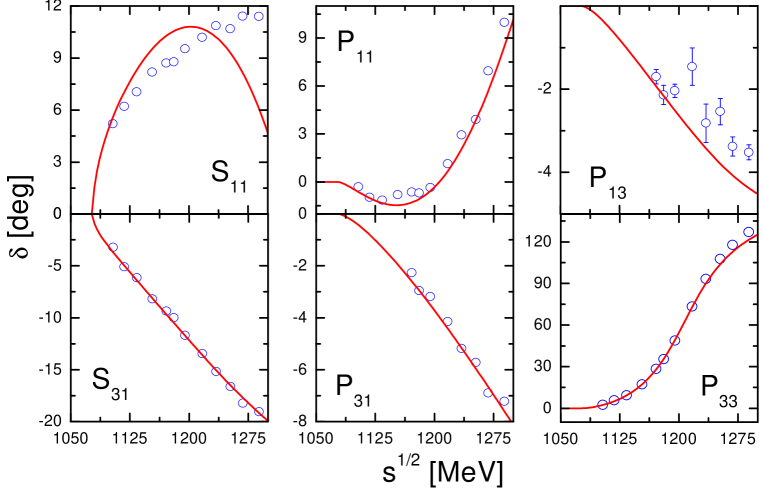
Figure 2: S- and p-wave pion-nucleon phase shifts. The single energy phase shifts are taken from [80].

5.5 $K^{+}$-nucleon scattering

We turn to the strangeness plus one channel. Since it is impossible to give here a comprehensive discussion of the many works dealing with kaon-nucleon scattering we refer to the review article by Dover and Walker [2] which is still up-to-date in many respects. The data situation can be summarized as follows: there exist precise low-energy differential cross sections for $K^{+}p$ scattering but no scattering data for the $K^{+}$-deuteron scattering process at low energies. Thus all low-energy results in the isospin zero channel necessarily follow from model-dependent extrapolations. We include the available differential cross section in our global fit. They are nicely reproduced as shown in Fig. 3. We include Coulomb interactions which are sizeable in the forward direction with $\cos\theta>0$.

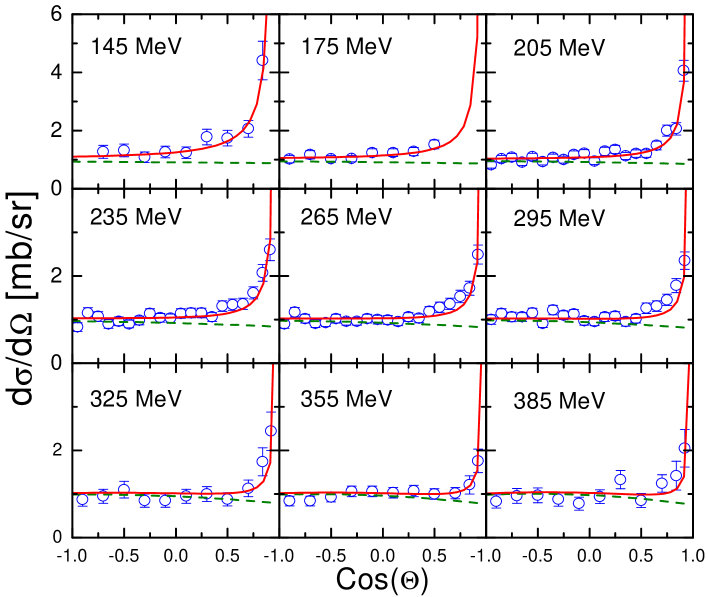
Figure 3: Differential cross section of $K^{+}$-proton scattering. The data points are taken from [108]. The solid lines give the result of the $\chi$-BS(3) analysis including Coulomb effects. The dashed lines follow for switched off Coulomb interaction.

It is instructive to consider the threshold amplitudes in detail. In the $\chi$-BS(3) approach the threshold parameters are determined by the threshold values of the effective interaction kernel $V^{(\pm)}_{KN}(m_{N}\!+\!m_{K};n)$ and the partial-wave loop function $J^{(\pm)}_{KN}(m_{N}\!+\!m_{K};n)$ (see (123,163)). Since all loop functions vanish at threshold but the one for the s-wave channel, all p-wave scattering volumes remain unchanged by the unitarization and are directly given by the threshold values of the appropriate effective interaction kernel $V_{KN}$. The explicit expressions for the scattering volumes to leading order can be found in Appendix H. In contrast the s-wave scattering lengths are renormalized strongly by the loop function $J^{(+)}_{KN}(m_{N}\!+\!m_{K};0)\neq 0$. At leading order the s-wave scattering lengths are

$$4\,\pi\left(1+\frac{m_{K}}{m_{N}}\right)a^{(KN)}_{S_{21}} = -m_{K}\left(f^{2}+\frac{m^{2}_{K}}{8\,\pi}\left(1-\frac{1}{\pi}\,\ln\frac{m_{K}^{2}}{m_{N}^{2}}\right)\right)^{-1}\;,$$

$$4\,\pi\left(1+\frac{m_{K}}{m_{N}}\right)a^{(KN)}_{S_{01}} = 0\;,$$ (176)

which lead to $a^{(KN)}_{S_{21}}\simeq-0.22$ fm and $a^{(KN)}_{S01}=0$ fm, close to our final values to subleading orders given in Tab. 15. In Tab. 15 we collected typical results for the p-wave scattering volumes also. The large differences in the isospin zero channel reflect the fact that this channel is not constrained by scattering data directly [2]. We find that some of our p-wave scattering volumes, also shown in Tab. 15, differ significantly from the values obtained by previous analyses. Such discrepancies may be explained in part by important cancellation mechanisms among the u-channel baryon octet and decuplet contributions (see Appendix H). An accurate description of the scattering volumes requires a precise input for the meson-baryon 3-point vertices. Since the $\chi$-BS(3) approach describes the 3-point vertices in accordance with all chiral constraints and large $N_{c}$ sum rules of QCD we believe our values for the scattering volumes to be rather reliable.

	$a^{(KN)}_{S_{01}}$ [fm]	$a^{(KN)}_{S_{21}}$ [fm]	$a^{(KN)}_{P_{01}}$ $[m_{\pi}^{-3}]$	$a^{(KN)}_{P_{21}}$ $[m_{\pi}^{-3}]$	$a^{(KN)}_{P_{03}}$ $[m_{\pi}^{-3}]$	$a^{(KN)}_{P_{23}}$ $[m_{\pi}^{-3}]$
$\chi$-BS(3)	0.06	-0.30	0.033	-0.017	-0.003	0.012
[109]	0.0	-0.33	0.028	-0.056	-0.046	0.025
[110]	-0.04	-0.32	0.030	-0.011	-0.007	0.007

Table 15: $K^{+}$-nucleon threshold parameters. The values of the $\chi$-BS(3) analysis are given in the first row. The last two rows recall the threshold parameters as given in [109] and [110].

In Fig. 4 we confront our s- and p-wave $K^{+}$-nucleon phase shifts with the most recent analyses by Hyslop et al. [109] and Hashimoto [79]. We find that our partial-wave phase shifts are reasonably close to the single energy phase shifts of [109] and [79] except the $P_{03}$ phase for which we obtain much smaller strength. Note however, that at higher energies we smoothly reach the single energy phase shifts of Hashimoto [79]. A possible ambiguity in that phase shift is already suggested by the conflicting scattering volumes found in that channel by earlier works (see Tab. 15). The isospin one channel, on the other hand, seems well-established even though the data set does not include polarization measurements close to threshold, which are needed to unambiguously determine the p-wave scattering volumes.

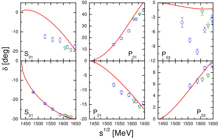
Figure 4: S- and p-wave $K^{+}$-nucleon phase shifts. The solid lines represent the results of the $\chi$-BS(3) approach. The open circles are from the Hyslop analysis [109] and the open triangles from the Hashimoto analysis [79].

5.6 $K^{-}$-nucleon scattering

We now turn to our results in the strangeness minus one sector. The antikaon-nucleon scattering process shows a large variety of intriguing phenomena. Inelastic channels are already open at threshold leading to a rich coupled-channel dynamics. Also the $\bar{K}N$ state couples to many of the observed hyperon resonances for which competing dynamical scenarios are conceivable. We fit directly the available data set rather than any partial wave analysis. Comparing for instance the energy dependent analyses [14] and [111] one finds large uncertainties in the s- and p-waves in particular at low energies. This reflects on the one hand a model dependence of the analysis and on the other hand an insufficient data set. A partial wave analysis of elastic and inelastic antikaon-nucleon scattering data without further constraints from theory is inconclusive at present [2, 112]. For a detailed overview of former theoretical analyses, we refer to the review article by Dover and Walker [2].

As motivated above we include the d-wave baryon resonance nonet field. An update of the analysis [38] leads to the estimates $F_{[9]}\simeq 1.8$, $D_{[9]}\simeq 0.84$ and $C_{[9]}\simeq 2.5$ for the resonance parameters. The singlet-octet mixing angle $\vartheta\simeq 28^{\circ}$ confirms the finding of [37], that the $\Lambda(1520)$ resonance is predominantly a flavor singlet state. By analogy with the expressions for the decuplet decay widths (47) of section 2 we apply the simple expressions

$$\Gamma_{N(1520)}=\frac{E_{N}-m_{N}}{16\,\pi\,f^{2}}\,\frac{p_{\pi N}^{3}}{m_{N(1520)}}\,\Big{(}F_{[9]}+D_{[9]}\Big{)}^{2}$$

$$\qquad\quad\;\,+\frac{E_{N}-m_{N}}{16\,\pi\,f^{2}}\,\frac{p_{\eta N}^{3}}{m_{N(1520)}}\,\Big{(}F_{[9]}-{\textstyle{1\over\sqrt{3}}}\,D_{[9]}\Big{)}^{2}\,,$$

$$\Gamma_{\Sigma(1680)}=\frac{E_{N}-m_{N}}{24\,\pi\,f^{2}}\,\frac{p_{\bar{K}N}^{3}}{m_{\Sigma(1680)}}\,\Big{(}F_{[9]}-D_{[9]}\Big{)}^{2}+\frac{E_{\Sigma}-m_{\Sigma}}{6\,\pi\,f^{2}}\,\frac{p_{\pi\Sigma}^{3}}{m_{\Sigma(1680)}}\,F_{[9]}^{2}$$

$$\qquad\quad\;\,+\frac{E_{\Lambda}-m_{\Lambda}}{36\,\pi\,f^{2}}\,\frac{p_{\pi\Lambda}^{3}}{m_{\Sigma(1680)}}\,D_{[9]}^{2}\,,$$

$$\Gamma_{\Xi(1820)}=\frac{E_{\Lambda}-m_{\Lambda}}{16\,\pi\,f^{2}}\,\frac{p_{\bar{K}\Lambda}^{3}}{m_{\Xi(1820)}}\,\Big{(}F_{[9]}-{\textstyle{1\over\sqrt{3}}}\,D_{[9]}\Big{)}^{2}$$

$$\qquad\quad\;\,+\frac{E_{\Sigma}-m_{\Sigma}}{16\,\pi\,f^{2}}\,\frac{p_{\bar{K}\Sigma}^{3}}{m_{\Xi(1820)}}\,\Big{(}F_{[9]}+D_{[9]}\Big{)}^{2}$$

$$\qquad\quad\;\,+\frac{E_{\Xi}-m_{\Xi}}{16\,\pi\,f^{2}}\,\frac{p_{\pi\Xi}^{3}}{m_{\Xi(1820)}}\,\Big{(}F_{[9]}-D_{[9]}\Big{)}^{2}\,,$$ (177)

where for example $E_{N}=\sqrt{m_{N}^{2}+p_{\pi N}^{2}}$ with the relative momentum $p_{\pi N}$ defined in the rest frame of the resonance. Our values for $F_{[9]}$ and $D_{[9]}$ describe the decay widths and branching ratios of the $\Sigma(1670)$ and $\Xi(1820)$ reasonably well within their large empirical uncertainties. Note that we put less emphasis on the properties of the $N(1520)$ resonance since that resonance is strongly influenced by the $\pi\Delta_{\mu}$ channel not considered here. In our global fit we take $F_{[9]}$ and $D_{[9]}$ fixed as given above but fine-tune the mixing angle $\vartheta=27.74^{\circ}$ and $C_{[9]}=2.509$. To account for further small inelastic three-body channels we assign the ’bare’ $\Lambda(1520)$ resonance an energy independent decay width of $\Gamma_{\Lambda(1520)}^{(3-{\rm body})}\simeq$ 1.4 MeV. The total cross sections are included in the fit for $p_{{\rm lab.}}<$ 500 MeV. For the bare masses of the d-wave resonances we use the values $m_{\Lambda(1520)}\simeq 1528.2$ MeV, $m_{\Lambda(1690)}\simeq 1705.3$ MeV and $m_{\Sigma(1680)}\simeq 1690.7$ MeV.

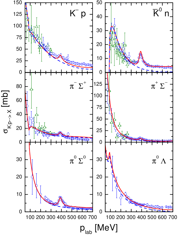
Figure 5: $K^{-}$-proton elastic and inelastic cross sections. The data are taken from [11, 13, 114, 115, 116, 117, 118, 119]. The solid lines show the results of our $\chi$-BS(3) theory including all effects of s-, p- and d-waves. The dashed lines represent the s-wave contributions only. We fitted the data points given by open circles [11, 13, 114, 115, 116, 117, 118]. Further data points represented by open triangles [119] were not considered in the global fit.

In Fig. 5 we present the result of our fit for the elastic and inelastic $K^{-}p$ cross sections. The data set is nicely reproduced including the rather precise data points for laboratory momenta 250 MeV$<p_{\rm lab}<$ 500 MeV. In Fig. 5 the s-wave contribution to the total cross section is shown with a dashed line. Important p-wave contributions are found at low energies only in the $\Lambda\pi^{0}$ production cross section. Note that the $\Lambda\pi^{0}$ channel carries isospin one and therefore provides valuable constraints on the poorly known $K^{-}$-neutron interaction. The deviation of our result from the empirical cross sections above $p_{\rm lab}\simeq 500$ MeV in some channels may be due in part to the fact that we do not consider the p-wave $\Lambda(1600)$ and $\Sigma(1660)$ resonances quantitatively in this work. As will be demonstrated below when presenting the partial-wave amplitudes, there is, however, a strong tendency that those resonances are generated in the $\chi$-BS(3) scheme. We checked that, by giving up some of the large $N_{c}$ sum rules and thereby increasing the number of free parameters we can easily obtain a fit with much improved quality beyond $p_{lab}=500$ MeV. We refrained from presenting those results because it is not clear that this procedure leads to the correct partial wave interpretation of the total cross sections. Note that the inelastic channel $K^{-}p\to\Lambda\pi\pi$, not included in this work, is no longer negligible at a quantitative level for $p_{\rm lab}>300$ MeV [113].

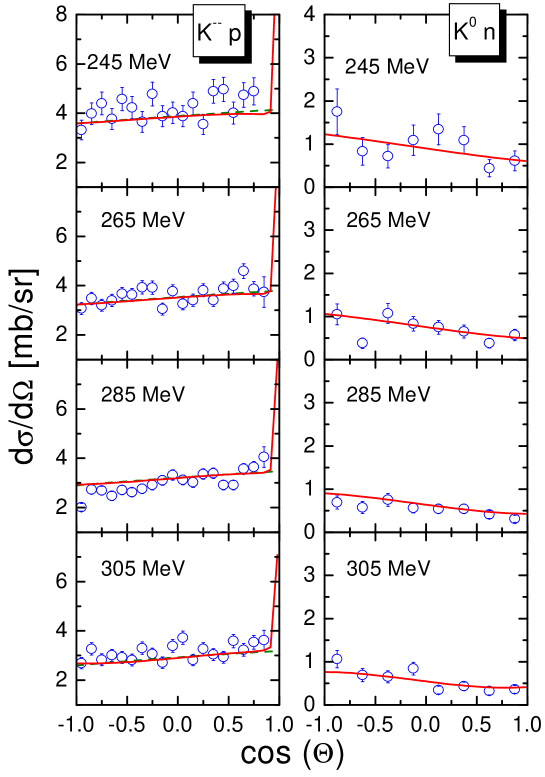
Figure 6: $K^{-}p\to K^{-}p,\,\bar{K}^{0}\,n$ differential cross sections at $p_{\rm lab}=245$ MeV, $265$ MeV, $285$ MeV and $305$ MeV. The data are taken form [116]. The solid lines represent our $\chi$-BS(3) theory including s-, p- and d-waves as well as Coulomb effects. The dashed lines follow if Coulomb interactions are switched off.

In Fig. 6 we confront our result with a selection of differential cross sections from elastic $K^{-}$-proton scattering [116]. The angular distribution patterns are consistent with weak p-wave interactions. The almost linear slope in $\cos\theta$ reflects the interference of the p-wave contribution with a strong s-wave. Coulomb effects are small in these channels. The differential cross sections provide valuable constraints on the p-wave interaction strengths.

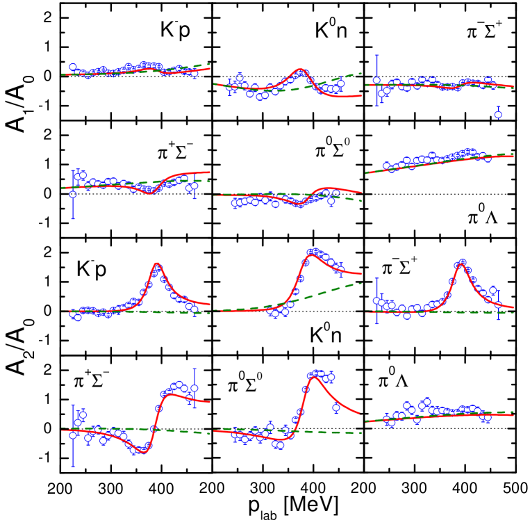
Figure 7: Coefficients $A_{1}$ and $A_{2}$ for the $K^{-}p\to\pi^{0}\Lambda$, $K^{-}p\to\pi^{\mp}\Sigma^{\pm}$ and $K^{-}p\to\pi^{0}\Sigma$ differential cross sections. The data are taken from [11, 117]. The solid lines are the result of the $\chi$-BS(3) approach with inclusion of the d-wave resonances. The dashed lines show the effect of switching off d-wave contributions.

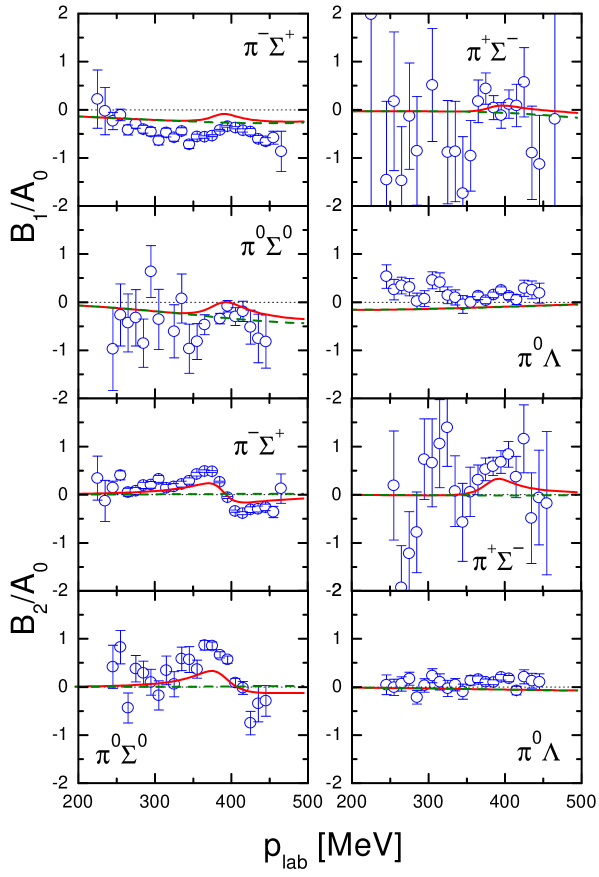
Figure 8: Coefficients $B_{1}$ and $B_{2}$ for the $K^{-}p\to\pi^{\mp}\Sigma^{\pm}$, $K^{-}p\to\pi^{0}\Sigma$ and $K^{-}p\to\pi^{0}\Lambda$ differential cross sections. The data are taken from [11, 117]. The solid lines are the result of the $\chi$-BS(3) approach with inclusion of the d-wave resonances. The dashed lines show the effect of switching off d-wave contributions.

Further important information on the p-wave dynamics is provided by angular distributions for the inelastic $K^{-}p$ reactions. The available data are represented in terms of coefficients $A_{n}$ and $B_{n}$ characterizing the differential cross section $d\sigma(\cos\theta,\sqrt{s}\,)$ and the polarization $P(\cos\theta,\sqrt{s}\,)$ as functions of the center of mass scattering angle $\theta$ and the total energy $\sqrt{s}$:

$$\frac{d\sigma(\sqrt{s},\cos\theta)}{d\cos\theta} = \sum_{n=0}^{\infty}A_{n}(\sqrt{s}\,)\,P_{n}(\cos\theta)\,,$$

$$\frac{d\sigma(\sqrt{s},\cos\theta)}{d\cos\theta}\,P(\sqrt{s},\cos\theta) = \sum_{n=1}^{\infty}B_{l}(\sqrt{s}\,)\,P^{1}_{n}(\cos\theta)\;.$$ (178)

In Fig. 7 we compare the empirical ratios $A_{1}/A_{0}$ and $A_{2}/A_{0}$ with the results of the $\chi$-BS(3) approach. Note that for $p_{\rm lab}<300$ MeV the empirical ratios with $n\geq 3$ are compatible with zero within their given errors. A large $A_{1}/A_{0}$ ratio is found only in the $K^{-}p\to\pi^{0}\Lambda$ channel demonstrating again the importance of p-wave effects in the isospin one channel. The dashed lines of Fig. 7, which are obtained when switching off d-wave contributions, confirm the importance of this resonance for the angular distributions in the isospin zero channel. The fact that the $\Lambda(1520)$ resonance appears more important in the differential cross sections than in the total cross sections follows simply because the tail of the resonance is enhanced if probed via an interference term. In the differential cross section the $\Lambda(1520)$ propagator enters linearly whereas the total cross section probes the squared propagator only. Note also the sizeable p-wave contributions at somewhat larger momenta seen in the charge-exchange reaction of Fig. 7 and also in Fig. 5.

The constraint from the ratios $B_{1}/A_{0}$ and $B_{2}/A_{0}$, presented in Fig. 8, is weak due to rather large empirical errors. New polarization data, possibly with polarized hydrogen targets, would be highly desirable.

	$a_{K^{-}p}$ [fm]	$a_{K^{-}n}$ [fm]	$\gamma$	$R_{c}$	$R_{n}$
Exp.	-0.78$\pm$0.18	-	2.36$\pm$ 0.04	0.664$\pm$0.011	0.189$\pm$0.015
	+$i$ (0.49$\pm$0.37)
$\chi$-BS(3)	-1.09+$i$ 0.82	0.29+$i$ 0.54	2.42	0.65	0.19
SU(2)	-0.79+$i$ 0.95	0.30+$i$ 0.49	4.58	0.63	0.32
	$a^{(\bar{K}N)}_{P_{01}}$ $[m_{\pi}^{-3}]$	$a^{(\bar{K}N)}_{P_{03}}$ $[m_{\pi}^{-3}]$		$a^{(\bar{K}N)}_{P_{21}}$ $[m_{\pi}^{-3}]$	$a^{(\bar{K}N)}_{P_{23}}$ $[m_{\pi}^{-3}]$
$\chi$-BS(3)	0.025+$i$ 0.001	0.002+$i$ 0.001		-0.004+$i$ 0.001	-0.055+$i$ 0.021

Table 16: $K^{-}$-nucleon threshold parameters. The row labelled by $SU(2)$ gives the results in the isospin limit with $m_{K^{-}}=m_{\bar{K}^{0}}=493.7$ MeV and $m_{p}=m_{n}=938.9$ MeV.

We turn to the threshold characteristics of the $K^{-}p$ reaction which is constrained by experimental data for the threshold branching ratios $\gamma,R_{c}$ and $R_{n}$ where

$$\gamma = \frac{\sigma(K^{-}\,p\rightarrow\pi^{+}\,\Sigma^{-})}{\sigma(K^{-}\,p\rightarrow\pi^{-}\,\Sigma^{+})}\;,\quad R_{c}=\frac{\sigma(K^{-}\,p\rightarrow\mbox{charged\,particles })}{\sigma(K^{-}\,p\rightarrow\mbox{all})}\;,$$

$$R_{n} = \frac{\sigma(K^{-}\,p\rightarrow\pi^{0}\,\Lambda)}{\sigma(K^{-}\,p\rightarrow\mbox{all\,neutral \,channels})}\;.$$ (179)

A further important piece of information is provided by the recent measurement of the $K^{-}$ hydrogen atom state which leads to a value for the $K^{-}p$ scattering length [5]. In Tab. 16 we confront the empirical numbers with our analysis. All threshold parameters are well described within the $\chi$-BS(3) approach. We confirm the result of [19, 20] that the branching ratios are rather sensitive to isospin breaking effects. However, note that it is sufficient to include isospin breaking effects only in the $\bar{K}N$ channel to good accuracy. The empirical branching ratios are taken from [10]. The real part of our $K^{-}n$ scattering length with $\Re\,a_{K^{-}n\to K^{-}n}\simeq 0.29$ fm turns out considerably smaller than the value of $0.53$ fm found in the recent analysis [20]. In Tab. 16 we present also our results for the p-wave scattering volumes. Here isospin breaking effects are negligible. All scattering volumes but the one in the $P_{23}$ channel are found to be small. The not too small and repulsive scattering volume $a_{P_{23}}\simeq(-0.16+i\,0.06)$ fm³ reflects the presence of the $\Sigma(1385)$ resonance just below the $\bar{K}N$ threshold. The precise values of the threshold parameters are of crucial importance when describing $K^{-}$-atom data which constitute a rather sensitive test of the in-medium dynamics of antikaons. In particular one expects a strong sensitivity of the level shifts to the s-wave scattering lengths.

In Fig. 9 we show the $\Lambda(1405)$ and $\Sigma(1385)$ spectral functions measured in the reactions $K^{-}p\rightarrow\Sigma^{+}\pi^{-}\pi^{+}\pi^{-}$ [120] and $K^{-}p\rightarrow\Lambda\pi^{+}\pi^{-}$ [121] respectively. We did not include the $\Lambda(1405)$ spectrum of [120] in our global fit. Since the $\Lambda(1405)$-spectrum shows a strong energy dependence, incompatible with a Breit-Wigner resonance shape, the spectral form depends rather strongly on the initial and final states through which it is measured. The empirical spectrum of [120] describes the reaction $\Sigma^{+}(1600)\,\pi^{-}\to\Lambda(1405)\to\Sigma^{+}\,\pi^{-}$ rather than the reactions $\Sigma^{\pm}\,\pi^{\mp}\to\Lambda(1405)\to\Sigma^{+}\,\pi^{-}$ accessible in our present scheme. In Fig. 6 the spectral form of the $\Lambda(1405)$ resulting from two different initial states $\Sigma^{\pm}\,\pi^{\mp}$ are confronted with the empirical spectrum of [120]. While the spectrum defined with respect to the initial state $\Sigma^{+}\,\pi^{-}$ represents the empirical spectrum reasonably well the other choice of initial state $\Sigma^{+}\,\pi^{-}$ leads to a significantly altered spectral form. We therefore conclude that in a scheme not including the $\Sigma(1600)\pi$ state explicitly it is not justified to use the $\Lambda(1405)$ spectrum of [120] as a quantitative constraint for the kaon-nucleon dynamics.

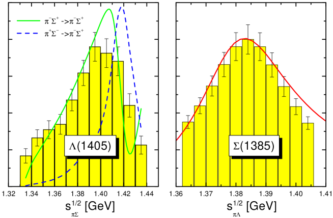
Figure 9: $\Lambda(1405)$ and $\Sigma(1385)$ resonance mass distributions in arbitrary units.

We turn to the mass spectrum of the decuplet $\Sigma(1385)$ state. The spectral form, to good accuracy of Breit-Wigner form, is reproduced reasonably well. Our result for the ratio of $\Sigma(1385)\to\pi\Lambda$ over $\Sigma(1385)\to\pi\Sigma$ of about $17\,\%$ compares well with the most recent empirical determination. In [122] that branching ratio was extracted from the $K^{-}p\to\Sigma(1385)\,K\,\bar{K}$ reaction and found to be $20\pm 6\,\%$. Note that we obtained our ratio from the two reaction amplitudes $\pi\Lambda\to\pi\Lambda$ and $\pi\Lambda\to\pi\Sigma$ evaluated at the $\Sigma(1385)$ pole. The schematic expression (47) would give a smaller value of about $15\,\%$. Finally we mention that the value for our $\Xi(1530)$ total width of $10.8$ MeV comfortably meets the empirical value of $9.9^{+1.7}_{-1.9}$ MeV given in [39].

5.7 Analyticity and crossing symmetry

It is important to investigate to what extent our multi-channel scattering amplitudes are consistent with the expectations from analyticity and crossing symmetry. As discussed in detail in section 4.3 the crossing symmetry constraints should not be considered in terms of partial-wave amplitudes, but rather in terms of the forward scattering amplitudes only. We expect crossing symmetry to be particularly important in the strangeness sector, because that sector has a large subthreshold region not directly accessible and constrained by data. In the following we reconstruct the forward $\bar{K}N$ and $KN$ scattering amplitudes in terms of their imaginary parts by means of dispersion integrals. We then confront the reconstructed scattering amplitudes with the original ones. It is non-trivial that those amplitudes match even though our loop functions and effective interaction kernels are analytic functions. One can not exclude that the coupled channel dynamics generates unphysical singularities off the real axis which would then spoil the representation of the scattering amplitudes in terms of dispersion integrals. Note that within effective field theory unphysical singularities are acceptable, however, only far outside the applicability domain of the approach.

Our analysis is analogous to that of Martin [6]. However, we consider the dispersion integral as a consistency check of our theory rather than as a predictive tool to derive the low-energy kaon-nucleon scattering amplitudes in terms of the more accurate scattering data at $E_{\rm lab}>300$ MeV [123]. This way we avoid any subtle assumptions on the number of required subtractions in the dispersion integral. Obviously the dispersion integral, if evaluated for small energies, must be dominated by the low-energy total cross sections which are not known empirically too well. We write a subtracted dispersion integral

$$\!\!T^{(0)}_{\bar{K}N}(s)=\frac{f^{2}_{KN\Lambda}}{s-m^{2}_{\Lambda}}+\sum_{k=1}^{n}\,c_{\bar{K}N}^{(0,k)}\,(s-s_{0})^{k}+\!\!\!\int_{(m_{\Sigma}+m_{\pi})^{2}}^{\infty}\!\!\!\!\frac{d\,s^{\prime}}{\pi}\,\frac{(s-s_{0})^{n}}{(s^{\prime}-s_{0})^{n}}\,\frac{\Im\,T^{(0)}_{\bar{K}N}(s^{\prime})}{s^{\prime}-s-i\,\epsilon}\;,$$

$$\!\!T^{(1)}_{\bar{K}N}(s)=\frac{f_{KN\Sigma}^{2}}{s-m^{2}_{\Sigma}}+\sum_{k=1}^{n}\,c_{\bar{K}N}^{(1,k)}\,(s-s_{0})^{k}+\!\!\!\int_{(m_{\Lambda}+m_{\pi})^{2}}^{\infty}\!\!\!\!\frac{d\,s^{\prime}}{\pi}\,\frac{(s-s_{0})^{n}}{(s^{\prime}-s_{0})^{n}}\,\frac{\Im\,T^{(1)}_{\bar{K}N}(s^{\prime})}{s^{\prime}-s-i\,\epsilon}\;,$$

$$\qquad\quad f_{KNY}=\sqrt{\frac{m_{K}^{2}-(m_{Y}-m_{N})^{2}}{2\,m_{N}}}\,\frac{m_{N}+m_{Y}}{2\,f}\,G^{(Y)}_{\bar{K}N}\,,$$ (180)

where we identify $s_{0}=\Lambda_{\rm opt.}^{2}=m_{N}^{2}+m_{K}^{2}$ with the optimal matching point of (164). We recall that the kaon-hyperon coupling constants $G^{(Y)}_{\bar{K}N}=A^{(Y)}_{\bar{K}N}+P^{(Y)}_{\bar{K}N}$ with $Y=\Lambda,\Sigma$ receive contributions from pseudo-vector and pseudo-scalar vertices as specified in Tab. 11. The values $f_{KN\Lambda}\simeq-12.8\,m^{1/2}_{\pi^{+}}$ and $f_{KN\Sigma}\simeq 6.1\,m^{1/2}_{\pi^{+}}$ follow.

The forward scattering amplitude $T_{\bar{K}N}(s)$ reconstructed in terms of the partial-wave amplitudes $f_{\bar{K}N,J}^{(L)}(\sqrt{s}\,)$ of (95) reads

$$T_{\bar{K}N}(s) = 4\,\pi\,\frac{\sqrt{s}}{m_{N}}\,\sum_{n=0}^{\infty}\,\Big{(}n+1\Big{)}\,\Big{(}f_{\bar{K}N,n+{\textstyle\frac{1}{2}}}^{(n)}(\sqrt{s}\,)+f_{\bar{K}N,n+{\textstyle\frac{1}{2}}}^{(n+1)}(\sqrt{s}\,)\Big{)}\;.$$ (181)

The subtraction coefficients $c_{\bar{K}N}^{(I,k)}$ are adjusted to reproduce the scattering amplitudes close to the kaon-nucleon threshold. One must perform a sufficient number of subtractions so that the dispersion integral in (180) is dominated by energies still within the applicability range of our theory. With $n=4$ in (180) we indeed find that we are insensitive to the scattering amplitudes for $\sqrt{s}>1600$ MeV to good accuracy. Similarly we write a subtracted dispersion integral for the amplitudes $T^{(I)}_{KN}(s)$ of the strangeness plus one sector

$$T^{(0)}_{KN}(s) = -\frac{1}{2}\,\frac{f^{2}_{KN\Lambda}}{2\,s_{0}-s-m^{2}_{\Lambda}}+\frac{3}{2}\,\frac{f^{2}_{KN\Sigma}}{2\,s_{0}-s-m^{2}_{\Sigma}}$$

$$+ \sum_{k=1}^{n}\,c_{KN}^{(0,k)}\,(s-s_{0})^{k}+\int_{(m_{N}+m_{K})^{2}}^{\infty}\frac{d\,s^{\prime}}{\pi}\,\frac{(s-s_{0})^{n}}{(s^{\prime}-s_{0})^{n}}\,\frac{\Im\,T^{(0)}_{KN}(s^{\prime})}{s^{\prime}-s-i\,\epsilon}\;,$$

$$T^{(1)}_{KN}(s) = \frac{1}{2}\,\frac{f^{2}_{KN\Lambda}}{2\,s_{0}-s-m^{2}_{\Lambda}}+\frac{1}{2}\,\frac{f^{2}_{KN\Sigma}}{2\,s_{0}-s-m^{2}_{\Sigma}}$$ (182)

$$+ \sum_{k=1}^{n}\,c_{KN}^{(1,k)}\,(s-s_{0})^{k}+\int_{(m_{N}+m_{K})^{2}}^{\infty}\frac{d\,s^{\prime}}{\pi}\,\frac{(s-s_{0})^{n}}{(s^{\prime}-s_{0})^{n}}\,\frac{\Im\,T^{(1)}_{KN}(s^{\prime})}{s^{\prime}-s-i\,\epsilon}\;.$$

The subtraction coefficients $c_{KN}^{(I,k)}$ are adjusted to reproduce the scattering amplitudes close to the kaon-nucleon threshold. The choice $n=4$ leads to a sufficient emphasis of the low-energy $KN$-amplitudes.

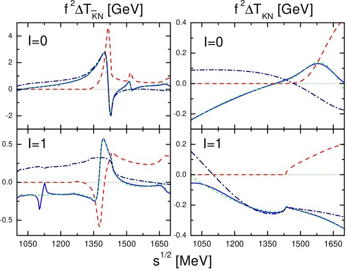
Figure 10: Causality check of the pole-subtracted kaon-nucleon scattering amplitudes $f^{2}\,\Delta T^{(I)}_{KN}$ and $f^{2}\,\Delta T^{(I)}_{\bar{K}N}$. The full lines represent the real part of the forward scattering amplitudes. The dotted lines give the amplitudes as obtained from their imaginary parts (dashed lines) in terms of the dispersion integrals (180) and (182). The dashed-dotted lines give the s-wave contribution to the real part of the forward scattering amplitudes only.

In Fig. 10 we compare the real part of the pole-subtracted amplitudes $\Delta T^{(I)}_{\bar{K}N}(s)$ and $\Delta T^{(I)}_{KN}(s)$ with the corresponding amplitudes reconstructed via the dispersion integral (180)

$$\Delta T_{\bar{K}N}^{(I)}(s) = T_{\bar{K}N}^{(I)}(s)-\frac{f^{2}_{KNY}}{s-m_{H}^{2}}-\left(A_{\bar{K}N}^{(Y)}\right)^{2}\frac{2\,m_{N}^{2}+m_{K}^{2}-s-m_{H}^{2}}{8\,f^{2}\,m_{N}}$$ (183)

$$+ \left(P_{\bar{K}N}^{(Y)}\right)^{2}\frac{(m_{N}+m_{H})^{2}}{8\,f^{2}\,m_{N}}+P_{\bar{K}N}^{(Y)}\,A_{\bar{K}N}^{(Y)}\frac{m^{2}_{H}-m_{N}^{2}}{4\,f^{2}\,m_{N}}\,,$$

with $Y=\Lambda$ for $I=0$ and $Y=\Sigma$ for $I=1$. Whereas it is straightforward to subtract the complete hyperon pole contribution in the $\bar{K}N$ amplitudes (see (183)), it is less immediate how to do so for the $KN$ amplitudes. Since we do not consider all partial wave contributions in the latter amplitudes the u-channel pole must be subtracted in its approximated form as given in (156). The reconstructed amplitudes agree rather well with the original amplitudes. For $\sqrt{s}>1200$ MeV the solid and dotted lines in Fig. 10 can hardly be discriminated. This demonstrates that our amplitudes are causal too good accuracy. Note that the discrepancy for $\sqrt{s}<1200$ MeV is a consequence of the approximate treatment of the non-local u-channel exchanges which violates analyticity at subthreshold energies to some extent (see (158)). With Fig. 10 we confirm that such effects are well controlled for $\sqrt{s}>1200$ MeV. In any case, close to $\sqrt{s}\simeq 1200$ MeV the complete forward scattering amplitudes are largely dominated by the s- and u-channel hyperon pole contributions absent in $\Delta T_{\bar{K}N}^{(I)}(s)$.

As can be seen from Fig. 10 also, we find sizeable p-wave contributions in the pole-subtracted amplitudes at subthreshold energies. This follows from comparing the dashed-dotted lines, which give the s-wave contributions only, with the solid lines which represent the complete real part of the pole-subtracted forward scattering amplitudes. The p-wave contributions are typically much larger below threshold than above threshold. The fact that this is not the case in the isospin zero $KN$ amplitude reflects a subtle cancellation mechanism of hyperon exchange contributions and quasi-local two-body interaction terms. In the $\bar{K}N$ amplitudes the subthreshold effects of p-waves are most dramatic in the isospin one channel. Here the amplitude is dominated by the $\Sigma(1385)$ resonance. Note that p-wave channels contribute with a positive imaginary part for energies larger than the kaon-nucleon threshold but with a negative imaginary part for subthreshold energies. A negative imaginary part of a subthreshold amplitude is consistent with the optical theorem which only relates the imaginary part of the forward scattering amplitudes to the total cross section for energies above threshold. Our analysis may shed some doubts on the quantitative results of the analysis by Martin, which attempted to constrain the forward scattering amplitude via a dispersion analysis [6]. An implicit assumption of Martin’s analysis was, that the contribution to the dispersion integral from the subthreshold region, which is not directly determined by the data set, is dominated by s-wave dynamics. As was pointed out in [21] strong subthreshold p-wave contributions should have an important effect for the propagation properties of antikaons in dense nuclear matter.

We turn to the approximate crossing symmetry of our scattering amplitudes. Crossing symmetry relates the subthreshold $\bar{K}N$ and $KN$ scattering amplitudes. As a consequence the exact amplitude ${\rm T}^{(0)}_{\bar{K}N}(s)$ shows unitarity cuts not only for $\sqrt{s}>m_{\Sigma}+m_{\pi}$ but also for $\sqrt{s}<m_{N}-m_{K}$ representing the elastic $KN$ scattering process. Consider for example the isospin zero amplitude for which one expects the following representation:

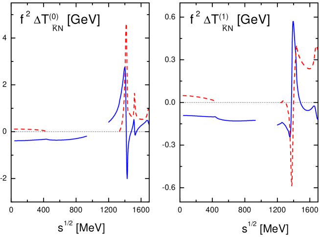
Figure 11: Approximate crossing symmetry of the pole subtracted kaon-nucleon forward scattering amplitudes. The lines in the left hand parts of the figures result from the $KN$ amplitudes. The lines in the right hand side of the figures give the $\bar{K}N$ amplitudes.

$$\!\!{\rm T}^{(0)}_{\bar{K}N}(s)-{\rm T}^{(0)}_{\bar{K}N}(s_{0}) = \frac{f^{2}_{KN\Lambda}}{s-m^{2}_{\Lambda}}-\frac{f^{2}_{KN\Lambda}}{s_{0}-m^{2}_{\Lambda}}+\!\!\!\int_{-\infty}^{(m_{N}-m_{K})^{2}}\frac{d\,s^{\prime}}{\pi}\,\frac{s-s_{0}}{s^{\prime}-s_{0}}\,\frac{\Im\,{\rm T}^{(0)}_{\bar{K}N}(s^{\prime})}{s^{\prime}-s-i\,\epsilon}$$ (184)

$$+ \int_{(m_{\Sigma}+m_{\pi})^{2}}^{+\infty}\frac{d\,s^{\prime}}{\pi}\,\frac{s-s_{0}}{s^{\prime}-s_{0}}\,\frac{\Im\,{\rm T}^{(0)}_{\bar{K}N}(s^{\prime})}{s^{\prime}-s-i\,\epsilon}\;,$$

where we performed one subtraction to help the convergence of the dispersion integral. Comparing the expressions for $T^{(0)}_{\bar{K}N}(s)$ in (180) and ${\rm T}^{(0)}_{\bar{K}N}(s)$ in (184) demonstrates that the contribution of the unitarity cut at $\sqrt{s}<m_{N}-m_{K}$ in (184) is effectively absorbed in the subtraction coefficients $c_{\bar{K}N}^{(I,k)}$ of (180). Similarly the subtraction coefficients $c_{KN}^{(I,k)}$ in (182) represent the contribution to $T^{(I)}_{KN}(s)$ from the inelastic $\bar{K}$N scattering process. Thus both model amplitudes $T^{(I)}_{KN}(s)$ and $T^{(I)}_{\bar{K}N}(s)$ represent the exact amplitude ${\rm T}^{(I)}_{\bar{K}N}(s)$ within their validity domains and therefore we expect approximate crossing symmetry

$$\Delta T^{(0)}_{\bar{K}N}(s)\simeq-\frac{1}{2}\,\Delta T^{(0)}_{KN}(2\,s_{0}-s)+\frac{3}{2}\,\Delta T^{(1)}_{KN}(2\,s_{0}-s)\;,$$

$$\Delta T^{(1)}_{\bar{K}N}(s)\simeq+\frac{1}{2}\,\Delta T^{(0)}_{KN}(2\,s_{0}-s)+\frac{1}{2}\,\Delta T^{(1)}_{KN}(2\,s_{0}-s)\;,$$ (185)

close to the optimal matching point $s_{0}=m_{N}^{2}+m_{K}^{2}$ only. In Fig. 11 we confront the pole-subtracted $\Delta T^{(I)}_{KN}$ and $\Delta T^{(I)}_{\bar{K}N}$ amplitudes with the expected approximate crossing identities (185). Since the optimal matching point $s_{0}=m_{N}^{2}+m_{K}^{2}\simeq(1068)^{2}$ MeV² is slightly below the respective validity range of the original amplitudes, we use the reconstructed amplitudes of (180) and (182) shown in Fig. 10. This is justified, because the reconstructed amplitudes are based on the imaginary parts of the amplitude which have support within the validity domain of our theory only. Fig. 11 indeed confirms that the kaon-nucleon scattering amplitudes are approximatively crossing symmetric. Close to the the point $s\simeq m_{N}^{2}+m_{K}^{2}$ the $KN$ and $\bar{K}N$ amplitudes match. We therefore expect that our subthreshold kaon-nucleon scattering amplitudes are determined rather reliably and well suited for an application to the nuclear kaon dynamics.

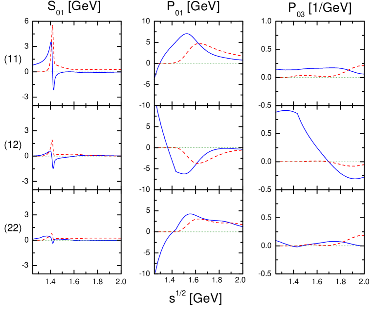
Figure 12: Real and imaginary parts of the s- and p-wave partial-wave amplitudes $f^{2}\,M$ in the isospin zero channel. The labels (ab) refer to our channel convention of (114) with (11): $\bar{K}N\to\bar{K}N$, (12): $\bar{K}N\to\pi\Sigma$ and (22): $\pi\Sigma\to\pi\Sigma$.

5.8 Scattering amplitudes

We discuss now the s- and p-wave partial-wave amplitudes for the various $\bar{K}N,\pi\Sigma$ and $\pi\Lambda$ reactions. Since we are interested in part also in subthreshold amplitudes we decided to present the invariant amplitudes $M^{(\pm)}(\sqrt{s},n)$ rather than the more common $f^{(l)}_{J}(\sqrt{s}\,)$ amplitudes. Whereas the latter amplitudes lead to convenient expressions for the cross sections

$$\sigma_{i\,\to f}(\sqrt{s}\,) = 4\,\pi\,\frac{p^{(f)}_{\rm cm}}{p^{(i)}_{\rm cm}}\,\sum_{l=0}^{\infty}\,\Bigg{(}l\,|f^{(l)}_{J=l-\frac{1}{2}}(\sqrt{s}\,)|^{2}+(l+1)\,|f^{(l)}_{J=l+\frac{1}{2}}(\sqrt{s}\,)|^{2}\Bigg{)}\;,$$ (186)

the former amplitudes $M^{(\pm)}(\sqrt{s},n)$ provide a more detailed picture of the higher partial-wave amplitudes, simply because the trivial phase-space factor $(p^{(f)}_{\rm cm}\,p^{(i)}_{\rm cm})^{l}$ is taken out

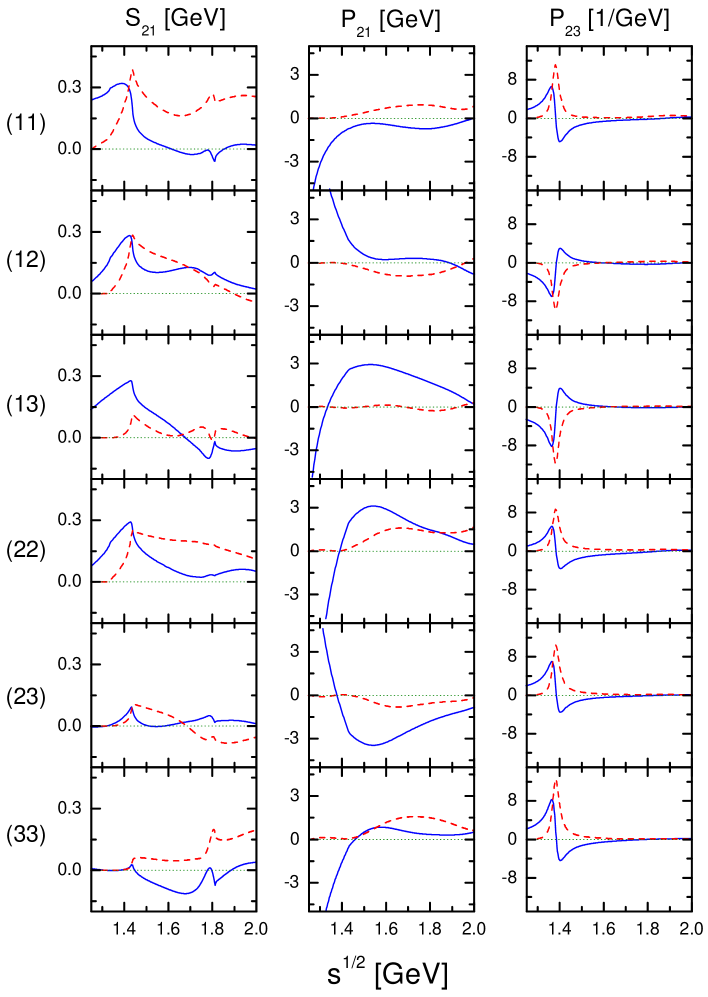
Figure 13: Real and imaginary parts of the s- and p-wave partial-wave amplitudes $f^{2}\,M$ in the isospin one channel. The labels (ab) refer to our channel convention of (114) with (11): $\bar{K}N\to\bar{K}N$, (12): $\bar{K}N\to\pi\Sigma$ and (13): $\bar{K}N\to\pi\Lambda$.

$$f^{(l)}_{J=l\pm\frac{1}{2}}(\sqrt{s}\,) = \frac{(p^{(f)}_{\rm cm}\,p^{(i)}_{\rm cm})^{J-\frac{1}{2}}}{8\,\pi\,\sqrt{s}}\;\sqrt{E_{i}\pm m_{i}}\,\sqrt{E_{f}\pm m_{f}}\,M^{(\pm)}(\sqrt{s},J-{\textstyle{1\over 2}})\;.$$ (187)

Here $p^{(i,f)}_{\rm cm}$ denote the relative momenta and $E_{i,f}$ the baryon energies in the center of mass frame. Also $m_{i,f}$ are the baryon masses of the initial and final baryons.

In Fig. 12 and in Fig.  13 the isospin zero and isospin one amplitudes are shown up to rather high energies $\sqrt{s}=2$ GeV. We emphasize that we trust our amplitudes quantitatively only up to $\sqrt{s}\simeq 1.6$ GeV. Beyond that energy one should consider our results as qualitative only. The amplitudes reflect the presence of the s-wave $\Lambda(1405)$ and p-wave $\Sigma(1385)$ resonances. From the relative height of the peak structures in the figures one can read off the branching ratios of those resonances. For instance it is clearly seen from Fig. 12 that the $\Lambda(1405)$ has a rather small coupling to the $\pi\Sigma$ channel. It is gratifying to find precursor effects for the p-wave $\Lambda(1600)$ and $\Lambda(1890)$ resonances in that figure also. Note that the estimates for the widths of those resonances range up to 200 MeV. Similarly Fig. 13 indicates attractive strength in the s- and p- wave channel where one would expect the s-wave $\Sigma(1750)$ and p-wave $\Sigma(1660)$ resonances.

It is a highly non-trivial but nevertheless expected result, that all resonances but the p-wave baryon decuplet and the d-wave baryon nonet resonances were generated dynamically by the chiral coupled channel dynamics once agreement with the low-energy data set with $p_{\rm lab.}<500$ MeV was achieved. A more accurate description of the latter resonances requires the extension of the $\chi$-BS(3) approach including more inelastic channels. These finding strongly support the conjecture that all baryon resonances but the decuplet ground states are a consequence of coupled-channels dynamics.

5.9 Predictions for cross sections

We close the result section by a presentation of total cross sections relevant for transport model calculation of heavy-ion reactions. We believe that the $\chi$-BS(3) approach is particularly well suited to determine some cross sections not directly accessible in scattering experiments. Typical examples would be the $\pi\Sigma\to\pi\Sigma,\pi\Lambda$ reactions. Here the quantitative realization of the chiral SU(3) flavor symmetry including its important symmetry breaking effects are an extremely useful constraint when deriving cross sections not accessible in the laboratory directly. It is common to consider isospin averaged cross sections [124, 125]

$$\bar{\sigma}(\sqrt{s}\,)=\frac{1}{N}\,\sum_{I}\,(2\,I+1)\,\sigma_{I}(\sqrt{s}\,)\,.$$ (188)

The reaction dependent normalization factor is determined by $N=\sum\,(2\,I+1)$ where the sum extends over isospin channels which contribute in a given reaction. In Fig. 14 we confront the cross sections of the channels $\bar{K}N,\pi\Sigma$ and $\pi\Lambda$. The results in the first row repeat to some extent the presentation of Fig. 5 only that here we confront the cross sections with typical parameterizations used in transport model calculations. The cross sections in the first column are determined by detailed balance from those of the first row. Uncertainties are present nevertheless, reflecting the large empirical uncertainties of the antikaon-nucleon cross sections close to threshold. The remaining four cross sections in Fig. 14 are true predictions of the $\chi$-BS(3) approach. Again we should emphasize that we trust our results quantitatively only for $\sqrt{s}<1600$ MeV. It is remarkable that nevertheless our cross sections agree with the parameterizations in [125] qualitatively up to much higher energies except in the $\bar{K}N\leftrightarrow\pi\Sigma$ reactions where we overshoot those parameterizations somewhat. Besides some significant deviations of our results from [124, 125] at $\sqrt{s}-\sqrt{s_{\rm th}}<$ 200 MeV, an energy range where we trust our results quantitatively, we find most interesting the sizeable cross section of about 30 mb for the $\pi\Sigma\to\pi\Sigma$ reaction. Note that here we include the isospin two contribution as part of the isospin averaging. As demonstrated by the dotted line in Fig. 14, which represent the $\chi$-BS(3) approach with s-wave contributions only, the p- and d-wave amplitudes are of considerable importance for the $\pi\Sigma\to\pi\Sigma$ reaction.

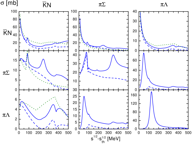
Figure 14: Total cross sections $\bar{K}N\to\bar{K}N$, $\bar{K}N\to\pi\Sigma$, $\bar{K}N\to\pi\Lambda$ etc relevant for subthreshold production of kaons in heavy-ion reactions. The solid and dashed lines give the results of the $\chi$-BS(3) approach with and without p- and d-wave contributions respectively. The dotted lines correspond to the parameterizations given in [125].

6 Summary and outlook

In this work we successfully used the relativistic chiral SU(3) Lagrangian to describe meson-baryon scattering. Within our $\chi$-BS(3) approach we established a unified description of pion-nucleon, kaon-nucleon and antikaon-nucleon scattering describing a large amount of empirical scattering data including the axial vector coupling constants for the baryon octet ground states. We derived the Bethe-Salpeter interaction kernel to chiral order $Q^{3}$ and then computed the scattering amplitudes by solving the Bethe-Salpeter equation. This leads to results consistent with covariance and unitarity. Moreover we consider the number of colors ($N_{c}$) in QCD as a large parameter performing a systematic $1/N_{c}$ expansion of the interaction kernel. This establishes a significant reduction of the number of parameters. Our analysis provides the first reliably estimates of previously poorly known s- and p-wave parameters. It is a highly non-trivial and novel result that the strength of all quasi-local 2-body interaction terms are consistent with the expectation from the large $N_{c}$ sum rules of QCD. Further intriguing results concern the meson-baryon coupling constants. The chiral $SU(3)$ flavor symmetry is found to be an extremely useful and accurate tool. Explicit symmetry breaking effects are quantitatively important but sufficiently small to permit an evaluation within chiral perturbation theory. We established two essential ingredients in a successful application of the chiral Lagrangian to the meson-baryon dynamics. First it is found that the explicit s- and u-channel decuplet contributions are indispensable for a good fit. Second, we find that it is crucial to employ the relativistic chiral Lagrangian. It gives rise to well defined kinematical structures in the quasi-local 4-point interaction terms which leads to a mixing of s-wave and p-wave parameters. Only in the heavy-baryon mass limit, not applied in this work, the parameters decouple into the s-wave and p-wave sector. In the course of developing our scheme we constructed a projector formalism which decouples in the Bethe-Salpeter equation covariant partial wave amplitudes and also suggested a minimal chiral subtraction scheme within dimensional regularization which complies manifestly with the chiral counting rules. An important test of our analysis could be provided by new data on kaon-nucleon scattering from the DA$\Phi$NE facility [1]. In particular additional polarization data, possibly with a polarized hydrogen or deuteron target, would be extremely useful.

We performed a consistency check of our forward scattering amplitudes by confronting them with their dispersion-integral representations. Our analysis shows that the scattering amplitudes are compatible with their expected analytic structure. Moreover we demonstrate that the kaon-nucleon and antikaon-nucleon scattering amplitudes are approximatively crossing symmetric in the sense that the $KN$ and $\bar{K}N$ amplitudes match at subthreshold energies. Our results for the $\bar{K}N$ amplitudes have interesting consequences for kaon propagation in dense nuclear matter as probed in heavy ion collisions [126]. According to the low-density theorem [127, 128] an attractive in-medium kaon spectral function probes the kaon-nucleon scattering amplitudes at subthreshold energies. The required amplitudes are well established in our work. In particular we find sizeable contributions from p-waves not considered systematically so far [129, 130, 131].

We expect our scattering amplitudes to lead to an improved description of the spectral functions of antikaons in nuclear matter and pave the way for a microscopic description of kaonic atom data. The latter are known to be a rather sensitive test of the antikaon-nucleon dynamics [132].

Appendices

Appendix A Isospin in $SU(3)$

The $SU(3)$ meson and baryon octet fields $\Phi=\sum\Phi_{i}\,\lambda_{i}$ and the baryon octet field $B=\sum B_{i}\,\lambda_{i}/\sqrt{2}$ with the Gell-Mann matrices $\lambda_{i}$ normalized by ${\rm tr}\,\lambda_{i}\,\lambda_{j}=2\,\delta_{ij}$ are decomposed into their isospin symmetric components

$$\Phi = \tau\cdot\pi+\alpha^{\dagger}\cdot K+K^{\dagger}\cdot\alpha+\eta\,\lambda_{8}\;,$$

$$B = {\textstyle{1\over\sqrt{2}}}\,\left(\tau\cdot\Sigma+\alpha^{\dagger}\cdot N+\Xi^{t}\,i\,\sigma_{2}\cdot\alpha+\lambda_{8}\,\Lambda\right)\,,$$

$$\alpha^{\dagger} = {\textstyle{1\over\sqrt{2}}}\left(\lambda_{4}+i\,\lambda_{5},\lambda_{6}+i\,\lambda_{7}\right)\;,\;\;\;\tau=(\lambda_{1},\lambda_{2},\lambda_{3})\;,$$ (189)

with the isospin singlet fields $\eta,\Lambda$, the isospin doublet fields $K=(K^{+},K^{0})^{t}$, $N=(p,n)^{t}$, $\Xi=(\Xi^{0},\Xi^{-})^{t}$ and the isospin triplet fields $\vec{\pi}=(\pi^{(1)},\pi^{(2)},\pi^{(3)})$, $\vec{\Sigma}=(\Sigma^{(1)},\Sigma^{(2)},\Sigma^{(3)})$. Similarly we derive the isospin decomposition of $(\bar{\Delta}_{\mu}\cdot\Phi)$, $(\Phi\cdot\Delta_{\mu})$ and $(\bar{\Delta}_{\mu}\cdot\Delta_{\nu})$ as defined in (14). The latter objects are expressed in terms of the isospin singlet field $\Omega^{-}$, the isospin doublet fields $\Xi_{\mu}=(\Xi^{0}_{\mu},\Xi^{-}_{\mu})^{t}$, the isospin triplet field $\vec{\Sigma}_{\mu}=(\Sigma^{(1)}_{\mu},\Sigma^{(2)}_{\mu},\Sigma^{(3)}_{\mu})$ and the isospin 3/2 field $\underline{\Delta}_{\mu}=(\Delta_{\mu}^{++},\Delta_{\mu}^{+},\Delta_{\mu}^{0},\Delta_{\mu}^{-})^{t}$. We find

$$\Big{(}\bar{\Delta}_{\mu}\cdot\Phi\Big{)}_{b}^{a} = \Big{(}\Big{(}\bar{\underline{\Delta}}_{\mu}\,S\,K\Big{)}\,\cdot\tau-\Big{(}\bar{\underline{\Delta}}_{\mu}\,S\,\alpha\Big{)}\,\cdot\pi-\frac{1}{\sqrt{6}}\,K^{\dagger}\,\Big{(}\bar{\Sigma}_{\mu}\cdot\sigma\Big{)}\,\alpha$$

$$+ \frac{1}{\sqrt{6}}\,\alpha^{\dagger}\,\Big{(}\bar{\Sigma}_{\mu}\cdot\sigma\Big{)}\,K+\frac{1}{\sqrt{2}}\,\Big{(}\bar{\Sigma}_{\mu}\cdot\pi\Big{)}\,\lambda_{8}-\frac{1}{\sqrt{2}}\,\Big{(}\bar{\Sigma}_{\mu}\cdot\tau\Big{)}\,\eta$$

$$- \frac{i}{\sqrt{6}}\,\Big{(}\bar{\Sigma}_{\mu}\times\pi\Big{)}\,\cdot\tau+\frac{1}{\sqrt{2}}\,\Big{(}K^{\dagger}\,i\,\sigma_{2}\,\bar{\Xi}_{\mu}^{t}\Big{)}\,\lambda_{8}-\frac{1}{\sqrt{6}}\,\Big{(}K^{\dagger}\,\sigma\,i\,\sigma_{2}\,\bar{\Xi}^{t}_{\mu}\Big{)}\,\cdot\tau$$

$$+ \frac{1}{\sqrt{6}}\,\alpha^{\dagger}\,\Big{(}\sigma\cdot\pi\Big{)}\,i\,\sigma_{2}\,\bar{\Xi}^{t}_{\mu}-\frac{1}{\sqrt{2}}\,\Big{(}\alpha^{\dagger}\,i\,\sigma_{2}\,\bar{\Xi}^{t}_{\mu}\Big{)}\,\eta$$

$$- \bar{\Omega}^{-}_{\mu}\,\Big{(}\alpha^{\dagger}\,i\,\sigma_{2}\,\Big{(}K^{\dagger}\Big{)}^{t}\Big{)}\Big{)}_{b}^{a}\;,$$

$$\Big{(}\Phi\cdot\Delta_{\mu}\Big{)}_{b}^{a} = \Big{(}\Big{(}K^{\dagger}\,S^{\dagger}\,{\underline{\Delta}}_{\mu}\Big{)}\,\cdot\tau-\Big{(}\alpha^{\dagger}\,S^{\dagger}\,{\underline{\Delta}}_{\mu}\Big{)}\,\cdot\pi-\frac{1}{\sqrt{6}}\,\alpha^{\dagger}\,\Big{(}\Sigma_{\mu}\cdot\sigma\Big{)}\,K$$ (190)

$$+ \frac{1}{\sqrt{6}}\,K^{\dagger}\,\Big{(}\Sigma\cdot\sigma\Big{)}\,\alpha+\frac{1}{\sqrt{2}}\,\Big{(}\Sigma_{\mu}\cdot\pi\Big{)}\,\lambda_{8}-\frac{1}{\sqrt{2}}\,\Big{(}\Sigma\cdot\tau\Big{)}\,\eta$$

$$+ \frac{i}{\sqrt{6}}\,\Big{(}\Sigma_{\mu}\times\pi\Big{)}\,\cdot\tau-\frac{1}{\sqrt{2}}\Big{(}\Xi^{t}_{\mu}\,i\,\sigma_{2}\,K\Big{)}\,\lambda_{8}+\frac{1}{\sqrt{6}}\,\Big{(}\Xi^{t}_{\mu}\,i\,\sigma_{2}\,\sigma\,K\Big{)}\,\cdot\tau$$

$$- \frac{1}{\sqrt{6}}\,\Xi^{t}\,\,i\,\sigma_{2}\,\Big{(}\sigma\cdot\pi\Big{)}\,\alpha+\frac{1}{\sqrt{2}}\,\Big{(}\Xi^{t}_{\mu}\,i\,\sigma_{2}\,\alpha\Big{)}\,\eta$$

$$+ \Omega^{-}_{\mu}\,\Big{(}K^{t}\,i\,\sigma_{2}\,\alpha\Big{)}\Big{)}_{b}^{a}$$

and

$$\Big{(}\bar{\Delta}_{\mu}\cdot\Delta_{\nu}\Big{)}_{b}^{a} = \Big{(}\frac{1}{2}\,\Big{(}\sum_{j}\,\bar{\underline{\Delta}}_{\mu}\,S_{j}\,\sigma\,S^{\dagger}_{j}\,{\underline{\Delta}}_{\nu}\Big{)}\,\cdot\tau+\frac{1}{6}\,\bar{\underline{\Delta}}_{\mu}\cdot{\underline{\Delta}}_{\nu}\,\Big{(}2+\sqrt{3}\,\lambda_{8}\Big{)}$$ (191)

$$+ \frac{1}{3}\,\bar{\Sigma}_{\mu}\cdot\Sigma_{\nu}+\frac{i}{3}\,\tau\cdot\Big{(}\bar{\Sigma}_{\mu}\times\Sigma_{\nu}\Big{)}$$

$$+ \frac{1}{6}\,\bar{\Xi}_{\mu}\,\Xi_{\nu}\,\Big{(}2-\sqrt{3}\,\lambda_{8}\Big{)}+\frac{1}{6}\,\Big{(}\bar{\Xi}_{\mu}\,\sigma\,\Xi_{\nu}\Big{)}\,\cdot\tau$$

$$+ \frac{1}{3}\,\bar{\Omega}^{-}_{\mu}\,\Omega^{-}_{\nu}\,\Big{(}1-\sqrt{3}\,\lambda_{8}\Big{)}$$

$$+ \frac{1}{\sqrt{6}}\,\bar{\underline{\Delta}}_{\mu}\,\Big{(}S\cdot\Sigma_{\nu}\Big{)}\,\alpha+\frac{1}{\sqrt{6}}\,\alpha^{\dagger}\,\Big{(}\bar{\Sigma}_{\mu}\cdot S^{\dagger}\Big{)}\,{\underline{\Delta}}_{\nu}$$

$$- \frac{1}{3}\,\bar{\Sigma}_{\mu}\cdot\,\Big{(}\Xi^{t}_{\nu}\,i\,\sigma_{2}\,\sigma\,\alpha\Big{)}+\frac{1}{3}\,\Big{(}\alpha^{\dagger}\,\sigma\,i\,\sigma_{2}\,\bar{\Xi}^{t}_{\mu}\Big{)}\,\cdot\Sigma_{\nu}$$

$$+ \frac{1}{\sqrt{6}}\,\bar{\Omega}^{-}_{\mu}\,\Big{(}\alpha^{\dagger}\,\Xi_{\nu}\Big{)}+\frac{1}{\sqrt{6}}\,\Big{(}\bar{\Xi}_{\mu}\,\alpha\Big{)}\,\Omega^{-}_{\nu}\Big{)}_{b}^{a}\;.$$

The isospin transition matrices $S_{i}$ are normalized by $S^{\dagger}_{i}\,S_{j}=\delta_{ij}-\sigma_{i}\,\sigma_{j}/3$. Note that the isospin Pauli matrices $\sigma_{i}$ act exclusively in the space of isospin doublet fields $K,N,\Xi,\Xi_{\mu}$ and the matrix valued isospin doublet $\alpha$. Expressions analogous to (190) hold for $(\bar{\Delta}_{\mu}\cdot B)$ and $(\bar{B}\cdot\Delta_{\mu})$.

The isospin reduction of the $SU(3)$ symmetric interaction terms is most conveniently derived applying the set of identities

$$\tau\cdot\alpha^{\dagger} = \alpha^{\dagger}\cdot\sigma\;,\;\;\;\;\;\alpha^{\dagger}\cdot\tau=0\;,\;\;\;\;\;\alpha\cdot\tau=\sigma\cdot\alpha\;,\;\;\;\;\;\tau\cdot\alpha=0\;,$$

$$\tau\,\lambda_{8} = \lambda_{8}\,\tau\;,\;\;\;\;\;{\rm tr}\,\big{(}\tau_{i}\,\tau_{j}\big{)}=2\,\delta_{ij}\;,\;\;\;\;{\rm tr}\,\big{(}\alpha_{i}\,\alpha^{\dagger}_{j}\big{)}=2\,\delta_{ij}\,,$$ (192)

where the $SU(2)$ Pauli matrices $\vec{\sigma}$ act exclusively on the isospin doublet fields. For example $\big{(}\vec{\sigma}\cdot\alpha\big{)}_{a}=\sum_{b}\,\vec{\sigma}_{ab}\,\alpha_{b}$. The algebra (192) is completed with

$$\Big{[}\alpha,\alpha^{\dagger}\Big{]}_{-} = -\tau\cdot\sigma-\sqrt{3}\,\lambda_{8}\;,\;\;\;\;\;\alpha\cdot\alpha=0\;,$$

$$\Big{[}\alpha\,,\alpha^{\dagger}\Big{]}_{+} = {\textstyle{4\over 3}}\,1-{\textstyle{1\over\sqrt{3}}}\,\lambda_{8}+\tau\cdot\sigma\;,\;\;\;\;\;\alpha^{\dagger}\cdot\alpha^{\dagger}=0\;,$$

$$\Big{[}\tau_{i}\,,\tau_{j}\Big{]}_{-} = 2\,i\,\epsilon_{ijk}\,\tau_{k}\;,\;\;\;\Big{[}\tau_{i}\,,\tau_{j}\Big{]}_{+}=\left({\textstyle{2\over\sqrt{3}}}\,\lambda_{8}+{\textstyle{4\over 3}}\,1\right)\delta_{ij}\;,$$

$$\Big{[}\lambda_{8}\,,\alpha^{\dagger}\Big{]}_{-} = \textstyle{\sqrt{3}}\,\alpha^{\dagger}\;,\;\;\;\;\Big{[}\lambda_{8}\,,\alpha^{\dagger}\Big{]}_{+}=-{\textstyle{1\over\sqrt{3}}}\,\alpha^{\dagger}\;,\;\;\;\;\Big{[}\lambda_{8}\,,\lambda_{8}\Big{]}_{+}={\textstyle{4\over 3}}\,1-{\textstyle{2\over\sqrt{3}}}\,\lambda_{8}\;,$$

$$\Big{[}\lambda_{8}\,,\alpha\,\Big{]}_{-} = -\textstyle{\sqrt{3}}\,\alpha\;,\;\;\;\Big{[}\lambda_{8}\,,\alpha\,\Big{]}_{+}=-{\textstyle{1\over\sqrt{3}}}\,\alpha\;,\;\;\;\Big{[}\lambda_{8}\,,\tau\Big{]}_{+}={\textstyle{2\over\sqrt{3}}}\,\tau\;$$ (193)

where $[A,B]_{\pm}=A\,B\pm B\,A$. By means of (192, 193) it is straightforward to derive the isospin structure of the chiral interaction terms. Note a typical intermediate result

$$\Big{[}\Phi,B\Big{]}_{+} = \sqrt{\frac{2}{3}}\,\Big{(}\lambda_{8}+\frac{2}{\sqrt{3}}\Big{)}\,\Big{(}\pi\cdot\Sigma\Big{)}+\frac{1}{\sqrt{2}}\,\pi\cdot\Big{(}\alpha^{\dagger}\,\sigma\,N\Big{)}+\sqrt{\frac{2}{3}}\,\tau\cdot\Big{(}\pi\,\Lambda\Big{)}$$ (194)

$$- \frac{1}{\sqrt{6}}\,\Big{(}\lambda_{8}-\frac{4}{\sqrt{3}}\Big{)}\,\Big{(}K^{\dagger}\,N\Big{)}+\frac{1}{\sqrt{2}}\,\tau\cdot\Big{(}K^{\dagger}\,\sigma\,N\Big{)}-\frac{1}{\sqrt{6}}\,\Big{(}K^{\dagger}\,\alpha\Big{)}\,\Lambda$$

$$+ \frac{1}{\sqrt{2}}\,\Big{(}K^{\dagger}\sigma\,\alpha\Big{)}\cdot\Sigma-\frac{1}{\sqrt{6}}\,\Big{(}\alpha^{\dagger}\,K\Big{)}\,\Lambda+\frac{1}{\sqrt{2}}\,\Big{(}\alpha^{\dagger}\,\sigma\,K\Big{)}\cdot\Sigma$$

$$- \sqrt{\frac{2}{3}}\,\Big{(}\lambda_{8}-\frac{2}{\sqrt{3}}\Big{)}\,\,\Big{(}\eta\,\Lambda\Big{)}-\frac{1}{\sqrt{6}}\,\eta\,\Big{(}\alpha^{\dagger}\,N\Big{)}+\sqrt{\frac{2}{3}}\,\tau\cdot\Big{(}\eta\,\Sigma\Big{)}$$

$$+ \frac{1}{\sqrt{2}}\,\pi\cdot\Big{(}\Xi^{t}\,i\,\sigma_{2}\,\sigma\,\alpha\Big{)}-\frac{1}{\sqrt{6}}\,\eta\,\Big{(}\Xi^{t}\,i\,\sigma_{2}\,\alpha\Big{)}$$

$$+ \frac{1}{\sqrt{2}}\,\tau\cdot\Big{(}\Xi^{t}\,i\,\sigma_{2}\,\sigma\,K\Big{)}-\frac{1}{\sqrt{6}}\,\Big{(}\lambda_{8}-\frac{4}{\sqrt{3}}\Big{)}\,\Big{(}\Xi^{t}\,i\,\sigma_{2}\,K\Big{)}\;.$$

Appendix B Local interaction terms of chiral order $Q^{3}$

For heavy-baryon chiral $SU(3)$ perturbation theory 102 terms of chiral order $Q^{3}$ are displayed in [82]. We find that only 10 chirally symmetric terms are relevant for elastic meson-baryon scattering. Following the constructing rules of Krause [35] one writes down 19 interaction terms for the relativistic chiral Lagrangian where terms which are obviously redundant by means of the equation of motion or $SU(3)$ trace identities [50] are not displayed. The Bethe-Salpeter interaction kernel (see (49)) receives the following contributions

$$K^{(I)}_{[8][8]}(\bar{k},k;w)=\frac{1}{8\,f^{2}}\,\Big{(}\big{(}\bar{p}\cdot\bar{q}\big{)}\big{(}p\cdot q\big{)}+\big{(}\bar{p}\cdot q\big{)}\big{(}p\cdot\bar{q}\big{)}\Big{)}\,C^{(I)}[h^{(1)}]$$ (195)

$$\qquad+\frac{1}{16\,f^{2}}\,\Big{(}q/\,\big{(}p-\bar{p}\big{)}\cdot\bar{q}-\bar{q}/\,\big{(}p-\bar{p}\big{)}\cdot q\Big{)}\,\bar{C}^{(I)}[h^{(2)}]$$

$$\qquad+\frac{1}{8\,f^{2}}\,\big{(}\bar{q}/+q/\big{)}\,(\bar{q}\cdot q)\,\,\bar{C}^{(I)}[h^{(3)}]$$

$$\qquad+\frac{1}{8\,f^{2}}\,i\,\gamma_{5}\,\gamma^{\mu}\,(p+\bar{p})^{\nu}\,\epsilon_{\mu\nu\alpha\beta}\,\bar{q}^{\alpha}\,q^{\beta}\,\bar{C}^{(I)}[h^{(4)}]$$

$$\qquad+\frac{1}{16\,f^{2}}\,i\,\gamma_{5}\,\gamma^{\mu}\,\Big{(}(\bar{p}\cdot(\bar{q}-q))\,p^{\mu}+(p\cdot(\bar{q}-q))\,\bar{p}^{\mu}\Big{)}\,\epsilon_{\mu\nu\alpha\beta}\,\bar{q}^{\alpha}\,q^{\beta}\,\bar{C}^{(I)}[h^{(5)}]$$

$$\qquad+\frac{1}{16\,f^{2}}\,i\,\gamma_{5}\,\gamma^{\mu}\,\Big{(}(\bar{p}\cdot(\bar{q}+q))\,p^{\mu}-(p\cdot(\bar{q}+q))\,\bar{p}^{\mu}\Big{)}\,\epsilon_{\mu\nu\alpha\beta}\,\bar{q}^{\alpha}\,q^{\beta}\,\bar{C}^{(I)}[h^{(6)}]\;,$$

where the interaction terms are already presented in momentum space for notational convenience. Their SU(3) structure is expressed in terms of the matrices $C_{0,1,D,F}$ and $\bar{C}_{1,D,F}$ introduced in (149). In (B) we applied the convenient notation:

$$\bar{C}^{(I)}[h^{(i)}] = h_{1}^{(i)}\,\bar{C}_{1}^{(I)}+h_{D}^{(i)}\,C_{D}^{(I)}+h_{F}^{(i)}\,C_{F}^{(I)}\,,$$

$$C^{(I)}[h^{(i)}] = h_{0}^{(i)}\,C_{0}^{(I)}+h_{1}^{(i)}\,C_{1}^{(I)}+h_{D}^{(i)}\,C_{D}^{(I)}+h_{F}^{(i)}\,C_{F}^{(I)}\,.$$ (196)

Explicit evaluation of the terms in (B) demonstrates that in fact only 10 terms contribute to the s and p- wave interaction kernels to chiral order $Q^{3}$. Obviously there are no quasi-local counter terms contributing to higher partial waves to this order. The terms of chiral order $Q^{2}$ are

$$V^{(I,+)}_{[8][8],2}(s;0) = \frac{s}{4\,f^{2}}\,\Big{(}\sqrt{s}-M^{(I)}\Big{)}\,C^{(I)}[h^{(1)}]\,\Big{(}\sqrt{s}-M^{(I)}\Big{)}\,,$$

$$V^{(I,-)}_{[8][8],2}(s;0) = \frac{1}{6\,f^{2}}\,M^{(I)}\,\Big{[}\,\bar{C}^{(I)}[h^{(4)}]\,,M^{(I)}\Big{]}_{+}\,M^{(I)}\,,$$

$$- \frac{1}{8\,f^{2}}\,\Big{(}\sqrt{s}+M^{(I)}\Big{)}\,\Big{[}\,\bar{C}^{(I)}[h^{(4)}]\,,M^{(I)}\Big{]}_{+}\,\Big{(}\sqrt{s}+M^{(I)}\Big{)}\,,$$

$$V^{(I,+)}_{[8][8],2}(s;1) = \frac{1}{24\,f^{2}}\,\Big{[}\,\bar{C}^{(I)}[h^{(4)}]\,,M^{(I)}\Big{]}_{+}\,.$$ (197)

We observe that the $h^{(1)}_{0,1,D,F}$ parameters can be absorbed into the $g^{(V)}_{0,1,D,F}$ to order $Q^{2}$ by the replacement $g^{(V)}\to g^{(V)}-M\,h^{(1)}$. Similarly the replacement $g^{(T)}\to g^{(T)}+M\,h^{(4)}$ cancels the dependence on $h^{(4)}$ at order $Q^{2}$ (see (151)). This mechanism illustrates the necessary regrouping of interaction terms required for the relativistic chiral Lagrangian as discussed in [26]. We turn to the quasi-local interaction terms of chiral order $Q^{3}$:

$$V^{(I,+)}_{[8][8],3}(s;0) = \frac{1}{8\,f^{2}}\,\,\Bigg{(}\Big{(}\phi^{(I)}+m_{\Phi(I)}^{2}\Big{)}\,\bar{C}^{(I)}[h^{(3)}]\,\Big{(}\sqrt{s}-M^{(I)}\Big{)}$$

$$\qquad+\Big{(}\sqrt{s}-M^{(I)}\Big{)}\,\bar{C}^{(I)}[h^{(3)}]\,\Big{(}\phi^{(I)}+m_{\Phi(I)}^{2}\Big{)}\Bigg{)}$$

$$-\frac{1}{4\,f^{2}}\!\!\! \!\!\!\Bigg{(}\frac{\phi^{(I)}}{2\,\sqrt{s}}\,\Big{(}C^{(I)}[g^{(S)}]+{\textstyle{1\over 2}}\,\sqrt{s}\,\bar{C}^{(I)}[h^{(2)}+2\,h^{(4)}]\Big{)}\,\Big{(}\sqrt{s}-M^{(I)}\Big{)}$$

$$+\!\!\! \!\!\!\Big{(}\sqrt{s}-M^{(I)}\Big{)}\,\Big{(}C^{(I)}[g^{(S)}]+{\textstyle{1\over 2}}\,\sqrt{s}\,\bar{C}^{(I)}[h^{(2)}+2\,h^{(4)}]\Big{)}\,\frac{\phi^{(I)}}{2\,\sqrt{s}}\Bigg{)}$$

$$-\frac{1}{4\,f^{2}}\!\!\! \!\!\!\Bigg{(}\frac{\phi^{(I)}}{2\,\sqrt{s}}\,\Big{(}\bar{C}^{(I)}[g^{(T)}]-{\textstyle{1\over 2}}\,\Big{[}\,\bar{C}^{(I)}[h^{(4)}]\,,M^{(I)}\Big{]}_{+}\Big{)}\,\Big{(}\sqrt{s}-M^{(I)}\Big{)}$$

$$+\!\!\! \!\!\!\Big{(}\sqrt{s}-M^{(I)}\Big{)}\,\Big{(}\bar{C}^{(I)}[g^{(T)}]-{\textstyle{1\over 2}}\,\Big{[}\,\bar{C}^{(I)}[h^{(4)}]\,,M^{(I)}\Big{]}_{+}\Big{)}\,\frac{\phi^{(I)}}{2\,\sqrt{s}}\Bigg{)}$$

$$- \frac{1}{8\,f^{2}}\,\,\Bigg{(}\Big{(}\phi^{(I)}+m_{\Phi(I)}^{2}\Big{)}\,C^{(I)}[g^{(V)}\!+\!2\,\sqrt{s}\,h^{(1)}]\,\Big{(}\sqrt{s}-M^{(I)}\Big{)}$$

$$\qquad+\Big{(}\sqrt{s}-M^{(I)}\Big{)}\,C^{(I)}[g^{(V)}\!+\!2\,\sqrt{s}\,h^{(1)}]\,\Big{(}\phi^{(I)}+m_{\Phi(I)}^{2}\Big{)}\Bigg{)}\,,$$

$$V^{(I,-)}_{[8][8],3}(s;0) = \frac{1}{8\,f^{2}}\,\sqrt{s}\,\Bigg{(}\Big{(}\sqrt{s}+M^{(I)}\Big{)}\,C^{(I)}[g^{(V)}]\,\Big{(}\sqrt{s}-M^{(I)}\Big{)}$$

$$\qquad\quad+\Big{(}\sqrt{s}-M^{(I)}\Big{)}\,C^{(I)}[g^{(V)}]\,\Big{(}\sqrt{s}+M^{(I)}\Big{)}\Bigg{)}$$

$$+ \frac{1}{12\,f^{2}}\,M^{(I)}\,\Big{[}\,C^{(I)}[g^{(V)}+2\,\sqrt{s}\,h^{(1)}]\,,\sqrt{s}-M^{(I)}\Big{]}_{+}\,M^{(I)}$$

$$+ \frac{1}{12\,f^{2}}\,M^{(I)}\,\Big{[}\,\bar{C}^{(I)}[h^{(2)}+2\,h^{(4)}-2\,h^{(3)}]\,,\sqrt{s}-M^{(I)}\Big{]}_{+}\,M^{(I)}\,,$$

$$V^{(I,+)}_{[8][8],3}(s;1) = \frac{1}{48\,f^{2}}\,\Big{[}\,C^{(I)}[g^{(V)}+2\,\sqrt{s}\,h^{(1)}]\,,\sqrt{s}-M^{(I)}\Big{]}_{+}$$ (198)

$$+ \frac{1}{48\,f^{2}}\,\Big{[}\,\bar{C}^{(I)}[h^{(2)}+2\,h^{(4)}-2\,h^{(3)}]\,,\sqrt{s}-M^{(I)}\Big{]}_{+}\,.$$

We observe that neither the $h^{(5)}$ nor the $h^{(6)}$ coupling constants enter the interaction kernel to chiral order $Q^{3}$. Furthermore the structure $h^{(4)}$ is redundant, because it disappears with the replacements to $g^{(T)}\to g^{(T)}+M\,h^{(4)}$ and $h^{(2)}\to h^{(2)}-2\,h^{(4)}$. Thus at chiral order $Q^{3}$ we find 10 relevant chirally symmetric parameters $h^{(1)}$, $h^{(2)}$ and $h^{(3)}$.

Appendix C Projector algebra

We establish the loop-orthogonality of the projectors ${Y}^{(\pm)}_{n}(\bar{q},q;w)$ introduced in (82). In order to facilitate our derivations we rewrite the projectors in terms of the convenient building objects $P_{\pm}$ and $V_{\mu}$ as

$${Y}^{(\pm)}_{n}(\bar{q},q;w)=\pm\,P_{\pm}\,\bar{Y}_{n+1}(\bar{q},q;w)\pm 3\,(\bar{q}\cdot V)\,P_{\mp}\,(V\cdot q)\,\bar{Y}_{n}(\bar{q},q;w)\;,$$

$$\bar{Y}_{n}(\bar{q},q;w)=\sum_{k=0}^{[(n-1)/2]}\,\frac{(-)^{k}\,(2\,n-2\,k)!}{2^{n}\,k!\,(n-k)!\,(n-2\,k-1)!}\,Y_{\bar{q}\bar{q}}^{k}\,Y_{\bar{q}q}^{n-2\,k-1}\,Y_{qq}^{k}\;,$$

$$Y_{ab}=\frac{(w\cdot a)\,(b\cdot w)}{w^{2}}-a\cdot b\,,\quad$$ (199)

where

$$P_{\pm}=\frac{1}{2}\left(1\pm\frac{w/}{\sqrt{w^{2}}}\right)\,,\quad V_{\mu}=\frac{1}{\sqrt{3}}\left(\gamma_{\mu}-\frac{w/}{w^{2}}\,w_{\mu}\right)\,,\quad P_{\pm}\,P_{\pm}=P_{\pm}\,,$$

$$P_{\pm}\,P_{\mp}=0\,,\quad P_{\pm}\,l/=l/\,P_{\mp}\pm(l\cdot w)/\sqrt{w^{2}}\,,\quad P_{\pm}\,V_{\mu}=V_{\mu}\,P_{\mp}\,.$$ (200)

In this appendix we will derive the identities:

$$\Im\ll n\,\pm|m\,\pm\gg(\bar{q},q;w)=\delta_{nm}\,Y^{(\pm)}_{n}(\bar{q},q;w)\,\Im J_{ab}^{(\pm)}(w;n)\;,$$

$$\Im\ll n\,\pm|m\,\mp\gg(\bar{q},q;w)=0\,,$$ (201)

with the convenient notation

$$\ll n\,\pm|m\,\pm\gg(\bar{q},q;w)=\int\frac{d^{4}l}{(2\pi)^{4}}\,Y^{(\pm)}_{n}(\bar{q},l;w)\,G(l;w)\,Y^{(\pm)}_{m}(l,q;w)\,,$$

$$G(l;w)=\frac{-i}{(w-l)^{2}-m_{a}^{2}+i\,\epsilon}\,\frac{l/+m_{b}}{l^{2}-m_{b}^{2}+i\,\epsilon}\,,$$

$$\Im\,J^{(\pm)}_{ab}(w;n)=\frac{p^{2\,n+1}_{ab}}{8\,\pi\,\sqrt{w^{2}}}\left(\frac{\sqrt{w^{2}}}{2}+\frac{m_{b}^{2}-m_{a}^{2}}{2\,\sqrt{w^{2}}}\pm m_{b}\right)\,,$$

$$\sqrt{w^{2}}=\sqrt{m_{a}^{2}+p^{2}}+\sqrt{m_{b}^{2}+p^{2}}\,.$$ (202)

The real parts of the loop functions $J_{ab}^{(\pm)}(w;n)$ are readily reconstructed by means of a dispersion integrals in terms of their imaginary parts. Since the loop functions are highly divergent they require a finite number of subtractions which are to be specified by the renormalization scheme. These terms are necessarily real and represent typically power divergent tadpole terms (see (88)). According to our renormalization condition (75) such terms must be moved into the effective interaction kernel.

In order to arrive at the desired result (201) we introduce further notation streamlining our derivation. For any covariant function $F(\bar{q},l,q;w)$ we write

$$\langle F\rangle_{n,m}(\bar{q},q;w)=\int\frac{d^{4}l}{(2\pi)^{4}}\,F(\bar{q},l,q;w)\,\bar{Y}_{n}(\bar{q},l;w)\,\bar{G}(l;w)\,\bar{Y}_{m}(l,q;w)\,,$$

$$\bar{G}(l;w)=\frac{1}{(w-l)^{2}-m_{a}^{2}+i\,\epsilon}\,\frac{-i}{l^{2}-m_{b}^{2}+i\,\epsilon}\,.$$ (203)

The result (201) is now derived in two steps. First the expressions in (201) are simplified by standard Dirac algebra methods. In the convenient notation of (203) we find

$$\ll n\,\pm|m\,\pm\gg = \langle m_{N}\pm(l\cdot\hat{w})\rangle_{n+1,m+1}\,P_{\pm}$$

$$+ 3\,\langle\big{(}m_{N}\pm(l\cdot\hat{w})\big{)}\,(l\cdot V)\rangle_{n+1,m}\,P_{\mp}\,(V\cdot q)$$

$$+ 3\,(\bar{q}\cdot V)\,P_{\mp}\,\langle(V\cdot l)\,\big{(}m_{N}\pm(l\cdot\hat{w})\big{)}\rangle_{n,m+1}$$

$$- 3\,(\bar{q}\cdot V)\,P_{\mp}\,\langle Y_{ll}\,\big{(}m_{N}\pm(l\cdot\hat{w})\big{)}\rangle_{n,m}\,(V\cdot q)\,,$$

$$\ll n\,\pm|m\,\mp\gg = -P_{\pm}\langle l/\rangle_{n+1,m+1}\,P_{\mp}+3\,(\bar{q}\cdot V)\,P_{\mp}\,\langle l/\,Y_{ll}\rangle_{n,m}\,P_{\pm}\,(V\cdot q)$$ (204)

$$+ P_{\pm}\,\langle\bar{q}/\,Y_{ll}\rangle_{n,m+1}\,P_{\mp}+P_{\pm}\,\langle q/\,Y_{ll}\rangle_{n+1,m}\,P_{\mp}\,,$$

where $\hat{w}_{\mu}=w_{\mu}/\sqrt{w^{2}}$. Next we observe that the terms $2\,(l\cdot w)=l^{2}-m_{b}^{2}-(w-l)^{2}+m_{a}^{2}+m_{b}^{2}-m_{a}^{2}+w^{2}$ and $Y_{ll}$ in (204) can be replaced by

$$l\cdot\hat{w}\to\frac{\sqrt{w^{2}}}{2}+\frac{m_{b}^{2}-m_{a}^{2}}{2\,\sqrt{w^{2}}}\,,\quad Y_{ll}\to p^{2}\,,$$ (205)

if tadpole contributions are neglected. The first replacement rule in (205) generates the typical structure occurring in (202). The final step consists in evaluating the remaining integrals. Consider for example the identities:

$$\langle 1\rangle_{n,m}(\bar{q},q;w)=\langle 1\rangle_{m,n}(q,\bar{q};w)=Y_{\bar{q}\bar{q}}^{(n-m)/2}\,\bar{Y}_{m}(\bar{q},q;w)\,J_{n+m-1}(w)\,,$$

$$\langle 1\rangle_{n+1,m}(\bar{q},q;w)=\langle 1\rangle_{m,n+1}(q,\bar{q};w)=0\,,\quad\Im\,J_{n}(w)=\frac{p^{n}}{8\pi\,\sqrt{w^{2}}}\,,$$ (206)

which hold modulo some subtraction polynomial for $n\geq m$ and both $n,m$ either even or odd. The result (206) is readily confirmed in the particular frame where $\vec{w}=0$

$$\bar{Y}_{n}(l,q;w)=\big{(}|\vec{l}\,|\,|\vec{q}\,|\big{)}^{n-1}\,P_{n}^{\prime}\big{(}\cos(\vec{l}\,,\vec{q}\,)\big{)}\,,$$ (207)

by applying the Cutkosky cutting rule in conjunction with standard properties of the Legendre polynomials. Here it is crucial to observe that the object $\bar{Y}_{n}(q,l;w)=\bar{Y}_{n}(l,q;w)$ does not exhibit any singularity in $l_{\mu}$. For example a square root term $\sqrt{Y_{\bar{q}l}}$ in $\bar{Y}(\bar{q},l;w)$ would invalidate our derivation. We point out that this observation leads to the unique interpretation of $P_{n}^{\prime}$ in terms of $Y_{qq}$, $Y_{\bar{q}\bar{q}}$ and $Y_{\bar{q}q}$ (see (207)) and thereby defines the unambiguous form of our projectors (199). Similarly one derives the identities:

$$\langle Y_{\bar{q}l}\rangle_{n+1,m}(\bar{q},q;w)=\langle Y_{\bar{q}l}\rangle_{m,n+1}(q,\bar{q};w)$$

$$\qquad\qquad\qquad\quad\quad=Y_{\bar{q}\bar{q}}\,Y_{\bar{q}\bar{q}}^{(n-m)/2}\,\bar{Y}_{m}(\bar{q},q;w)\,J_{n+m+1}(w)\,,$$

$$\langle Y_{lq}\rangle_{n+1,m}(\bar{q},q;w)=\langle Y_{lq}\rangle_{m,n+1}(q,\bar{q};w)$$

$$\qquad\qquad\qquad\quad\quad=Y_{\bar{q}q}\,Y_{\bar{q}\bar{q}}^{(n-m)/2}\,\bar{Y}_{m}(\bar{q},q;w)\,J_{n+m+1}(w)\,,$$

$$\langle Y_{\bar{q}l}\rangle_{n,m}(\bar{q},q;w)=\langle Y_{\bar{q}l}\rangle_{m,n}(q,\bar{q};w)=0\,,$$

$$\langle Y_{lq}\rangle_{n,m}(\bar{q},q;w)=\langle Y_{lq}\rangle_{m,n}(q,\bar{q};w)=0\,,$$ (208)

which again hold modulo some subtraction polynomial for $n\geq m$ and both $n,m$ either even or odd. Our proof of (201) is completed with the convenient identities:

$$\langle l_{\mu}\rangle_{n+1,m}=\hat{w}_{\mu}\,\langle Y_{ll}\,(l-\bar{q})\cdot\hat{w}\rangle_{n,m}+\bar{q}_{\mu}\,\langle Y_{ll}\rangle_{n,m}\quad{\rm if\;n\geq m}\;,$$

$$Y_{qq}\,\langle l_{\mu}\rangle_{n+1,m}=\hat{w}_{\mu}\,\langle(l-q)\cdot\hat{w}\rangle_{n+1,m+1}+q_{\mu}\,\langle 1\rangle_{n+1,m+1}\quad{\rm if\;n<m}\;,$$

$$\langle l_{\mu}\rangle_{n,m+1}=\hat{w}_{\mu}\,\langle Y_{ll}\,(l-q)\cdot\hat{w}\rangle_{n,m}+q_{\mu}\,\langle Y_{ll}\rangle_{n,m}\quad{\rm if\;n\leq m}\;,$$

$$Y_{\bar{q}\bar{q}}\,\langle l_{\mu}\rangle_{n,m+1}=\hat{w}_{\mu}\,\langle(l-\bar{q})\cdot\hat{w}\rangle_{n+1,m+1}+\bar{q}_{\mu}\,\langle 1\rangle_{n+1,m+1}\quad{\rm if\;n>m}\;,$$ (209)

which follow from (208) and covariance which implies the replacement rule

$$l_{\mu}\to\frac{Y_{q\bar{q}}\,Y_{\bar{q}l}-Y_{\bar{q}\bar{q}}\,Y_{ql}}{Y_{q\bar{q}}^{2}-Y_{qq}\,Y_{\bar{q}\bar{q}}}\,\left(q_{\mu}-\frac{w\cdot q}{w^{2}}\,w_{\mu}\right)$$

$$\quad+\frac{Y_{q\bar{q}}\,Y_{ql}-Y_{qq}\,Y_{\bar{q}l}}{Y_{q\bar{q}}^{2}-Y_{qq}\,Y_{\bar{q}\bar{q}}}\,\left(\bar{q}_{\mu}-\frac{w\cdot\bar{q}}{w^{2}}\,w_{\mu}\right)+\frac{l\cdot w}{w^{2}}\,w_{\mu}\,.$$ (210)

The identities (201) follow now from (204) and (209). For example, the first identity follows for $n=m$, because the first two terms in (204) lead to the loop function $J_{ab}^{(\pm)}(w;n)$ and the last two terms cancel. Similarly for $n>m$ the first and second terms are canceled by the third and fourth terms respectively whereas for $n<m$ both, the first two and last two terms in (204) cancel separately.

Appendix D Isospin breaking effects

Isospin breaking effects are easily incorporated by constructing super matrices $V^{(I^{\prime}I)},J^{(I^{\prime}I)}$ and $T^{(I^{\prime}I)}$ which couple different isospin states. Here we only consider isospin breaking effects induced by the loop functions, i.e. the interaction kernel $V^{(I^{\prime}I)}=\delta_{I^{\prime}I}\,V^{(I)}$ is assumed isospin diagonal.

Furthermore we neglect isospin breaking effects in all but the s-wave $\bar{K}N$-channels. This leads to

$$J_{\bar{K}N}^{(00)}=J_{\bar{K}N}^{(11)}=\frac{1}{2}\Big{(}J_{K^{-}p}+J_{\bar{K^{0}}n}\Big{)}\,,\,\,J_{\bar{K}N}^{(01)}=J_{\bar{K}N}^{(10)}=\frac{1}{2}\Big{(}J_{K^{-}p}-J_{\bar{K^{0}}n}\Big{)}\,.$$ (211)

The remaining channels $X$ are defined via $J^{(I^{\prime}I)}_{X}=\delta_{I^{\prime}I}\,J^{(I)}_{X}$ with isospin averaged masses in the loop functions. We use also isospin averaged meson and baryon masses in $V^{(I)}$. Note that there is an ambiguity in the subtraction point of the isospin transition loop function $J_{\bar{K}N}^{(01)}$. We checked that taking $m_{\Lambda}$ as used for $J_{\bar{K}N}^{(00)}$ or $m_{\Sigma}$ as used for $J_{\bar{K}N}^{(11)}$ makes little difference. We use the average hyperon mass $(m_{\Lambda}+m_{\Sigma})/2$. The $K^{-}p$-reaction matrices can now be linearly combined in terms of appropriate matrix elements of $M^{(I^{\prime}I)}$

$$M_{K^{-}\,p\,\rightarrow K^{-}\,p\;} = \frac{1}{2}\,M^{I=(0,0)}_{\bar{K}N\rightarrow\bar{K}N}+\frac{1}{2}\,M^{I=(1,1)}_{\bar{K}N\rightarrow\bar{K}N}+\frac{1}{2}\,M^{I=(0,1)}_{\bar{K}N\rightarrow\bar{K}N}+\frac{1}{2}\,M^{I=(1,0)}_{\bar{K}N\rightarrow\bar{K}N}\;,$$

$$M_{K^{-}\,p\,\rightarrow\bar{K}^{0}\;n\;} = \frac{1}{2}\,M^{I=(0,0)}_{\bar{K}N\rightarrow\bar{K}N}-\frac{1}{2}\,M^{I=(1,1)}_{\bar{K}N\rightarrow\bar{K}N}-\frac{1}{2}\,M^{I=(0,1)}_{\bar{K}N\rightarrow\bar{K}N}+\frac{1}{2}\,M^{I=(1,0)}_{\bar{K}N\rightarrow\bar{K}N}\;,$$

$$M_{K^{-}\,p\,\rightarrow\pi^{-}\Sigma^{+}\!} = \frac{1}{\sqrt{6}}\,M^{I=(0,0)}_{\bar{K}N\rightarrow\pi\Sigma}+\frac{1}{2}\,M^{I=(1,1)}_{\bar{K}N\rightarrow\pi\Sigma}+\frac{1}{\sqrt{6}}\,M^{I=(1,0)}_{\bar{K}N\rightarrow\pi\Sigma}+\frac{1}{2}\,M^{I=(0,1)}_{\bar{K}N\rightarrow\pi\Sigma}\;,$$

$$M_{K^{-}\,p\,\rightarrow\pi^{+}\Sigma^{-}\!} = \frac{1}{\sqrt{6}}\,M^{I=(0,0)}_{\bar{K}N\rightarrow\pi\Sigma}-\frac{1}{2}\,M^{I=(1,1)}_{\bar{K}N\rightarrow\pi\Sigma}+\frac{1}{\sqrt{6}}\,M^{I=(1,0)}_{\bar{K}N\rightarrow\pi\Sigma}-\frac{1}{2}\,M^{I=(0,1)}_{\bar{K}N\rightarrow\pi\Sigma}\;,$$

$$M_{K^{-}\,p\,\rightarrow\pi^{0}\,\Sigma\;} = \frac{1}{\sqrt{6}}\,M^{I=(0,0)}_{\bar{K}N\rightarrow\pi\Sigma}+\frac{1}{\sqrt{6}}\,M^{I=(1,0)}_{\bar{K}N\rightarrow\pi\Sigma}\;,$$

$$M_{K^{-}\,p\,\rightarrow\,\pi^{0}\,\Lambda\;} = \frac{1}{\sqrt{2}}\,M^{I=(0,1)}_{\bar{K}N\rightarrow\pi\Lambda}+\frac{1}{\sqrt{2}}\,M^{I=(1,1)}_{\bar{K}N\rightarrow\pi\Lambda}\;.$$ (212)

The $K^{+}p\to K^{+}p$ reaction of the strangeness +1 channel remains a single channel problem due to charge conservation. One finds

$$M_{K^{+}\,p\,\rightarrow K^{+}\,p\;} = M^{I=(1,1)}_{KN\rightarrow KN}\;,\quad J_{KN}^{(11)}=J_{K^{+}p}\;.$$ (213)

The charge exchange reaction $K^{+}n\to K^{0}p$, on the other hand, turns into a 2 channel problem with ($K^{+}n$, $K^{0}p$). The proper matrix structure in the isospin basis leads to

$$M_{K^{+}\,n\,\rightarrow K^{0}\,p\;}=\frac{1}{2}\,M^{I=(1,1)}_{KN\rightarrow KN}-\frac{1}{2}\,M^{I=(0,0)}_{KN\rightarrow KN}+\frac{1}{2}\,M^{I=(0,1)}_{KN\rightarrow KN}+\frac{1}{2}\,M^{I=(1,0)}_{KN\rightarrow KN}\;,$$

$$J_{KN}^{(00)}=J_{KN}^{(11)}=\frac{1}{2}\,\Big{(}J_{K^{+}n}+J_{K^{0}p}\Big{)}\;,\;\;J_{KN}^{(01)}=J_{KN}^{(10)}=\frac{1}{2}\,\Big{(}J_{K^{+}n}-J_{K^{0}p}\Big{)}\;.$$ (214)

The subtraction point $\mu^{(I)}$ in the loop functions $J_{K^{+}p},J_{K^{+}n}$ and $J_{K^{0}p}$ is identified with the average hyperon mass $\mu^{(0)}=\mu^{(1)}=(m_{\Lambda}+m_{\Sigma})/2$.

Appendix E Strangeness minus one channel

We collect the coefficients $C^{(I)}_{...}$ defined in (143,131,149) in Tab. 17 and Tab. 18. For completeness we also include the $I=2$ channel. All coefficients are defined within the natural extension of our notation in (114). The appropriate isospin states $R^{(2)}$ are introduced as

$$R^{(2)}_{[n]}=\pi_{c}\cdot S_{[n]}\cdot\Sigma\,,\qquad$$ (215)

where the matrix valued vector $S_{[n]}$ satisfies

$$\sum_{n=1}^{5}\,S^{\dagger}_{[n],\,ac}\,S^{\,}_{[n],\,bd}={\textstyle{1\over 2}}\,\delta_{ab}\,\delta_{cd}+{\textstyle{1\over 2}}\,\delta_{ad}\,\delta_{cb}-{\textstyle{1\over 3}}\,\delta_{ac}\,\delta_{bd}\,.$$ (216)

	$C_{WT}^{(0)}$	$C_{N_{[8]}}^{(0)}$	$C_{\Lambda_{[8]}}^{(0)}$	$C_{\Sigma_{[8]}}^{(0)}$	$C_{\Delta_{[10]}}^{(0)}$	$C_{\Sigma_{[10]}}^{(0)}$	$\widetilde{C}_{N_{[8]}}^{(0)}$	$\widetilde{C}_{\Lambda_{[8]}}^{(0)}$	$\widetilde{C}_{\Sigma_{[8]}}^{(0)}$	$\widetilde{C}_{\Xi_{[8]}}^{(0)}$	$\widetilde{C}_{\Delta_{[10]}}^{(0)}$	$\widetilde{C}_{\Sigma_{[10]}}^{(0)}$	$\widetilde{C}_{\Xi_{[10]}}^{(0)}$
$11$	$3$	0	$1$	$0$	0	0	0	0	0	0	0	0	0
$12$	$\sqrt{\frac{3}{2}}$	0	$1$	$0$	0	0	$\sqrt{\frac{2}{3}}$	0	0	0	$2\sqrt{\frac{2}{3}}$	0	0
$13$	$\frac{3}{\sqrt{2}}$	0	$1$	$0$	0	0	$\sqrt{2}$	0	0	0	0	0	0
$14$	$0$	0	$1$	$0$	0	0	0	$\frac{1}{2}$	-$\frac{3}{2}$	0	0	-$\frac{3}{2}$	0
$22$	$4$	0	$1$	$0$	0	0	0	$\frac{1}{3}$	-1	0	0	-1	0
$23$	$0$	0	$1$	$0$	0	0	0	0	$\sqrt{3}$	0	0	$\sqrt{3}$	0
$24$	-$\sqrt{\frac{3}{2}}$	0	$1$	$0$	0	0	0	0	0	-$\sqrt{\frac{2}{3}}$	0	0	-$\sqrt{\frac{2}{3}}$
$33$	$0$	0	$1$	$0$	0	0	0	1	0	0	0	0	0
$34$	-$\frac{3}{\sqrt{2}}$	0	$1$	$0$	0	0	0	0	0	-$\sqrt{2}$	0	0	-$\sqrt{2}$
$44$	$3$	0	$1$	$0$	0	0	0	0	0	0	0	0	0
	$C_{WT}^{(1)}$	$C_{N_{[8]}}^{(1)}$	$C_{\Lambda_{[8]}}^{(1)}$	$C_{\Sigma_{[8]}}^{(1)}$	$C_{\Delta_{[10]}}^{(1)}$	$C_{\Sigma_{[10]}}^{(1)}$	$\widetilde{C}_{N_{[8]}}^{(1)}$	$\widetilde{C}_{\Lambda_{[8]}}^{(1)}$	$\widetilde{C}_{\Sigma_{[8]}}^{(1)}$	$\widetilde{C}_{\Xi_{[8]}}^{(1)}$	$\widetilde{C}_{\Delta_{[10]}}^{(1)}$	$\widetilde{C}_{\Sigma_{[10]}}^{(1)}$	$\widetilde{C}_{\Xi_{[10]}}^{(1)}$
$11$	1	0	0	1	0	1	0	0	0	0	0	0	0
$12$	1	0	0	1	0	1	-$\frac{2}{3}$	0	0	0	$\frac{2}{3}$	0	0
$13$	$\sqrt{\frac{3}{2}}$	0	$0$	$1$	0	1	$\sqrt{\frac{2}{3}}$	0	0	0	0	0	0
$14$	$\sqrt{\frac{3}{2}}$	0	$0$	$1$	0	1	$\sqrt{\frac{2}{3}}$	0	0	0	0	0	0
$15$	$0$	0	$0$	$1$	0	1	0	-$\frac{1}{2}$	-$\frac{1}{2}$	0	0	-$\frac{1}{2}$	0
$22$	$2$	0	$0$	$1$	0	1	0	-$\frac{1}{3}$	$\frac{1}{2}$	0	0	$\frac{1}{2}$	0
$23$	$0$	0	$0$	$1$	0	1	0	0	-1	0	0	-1	0
$24$	$0$	0	$0$	$1$	0	1	0	0	1	0	0	1	0
$25$	$-1$	0	$0$	$1$	0	1	0	0	0	$\frac{2}{3}$	0	0	$\frac{2}{3}$
$33$	$0$	0	$0$	$1$	0	1	0	0	1	0	0	1	0
$34$	$0$	0	$0$	$1$	0	1	0	$\frac{1}{\sqrt{3}}$	0	0	0	0	0
$35$	$\sqrt{\frac{3}{2}}$	0	$0$	$1$	0	1	0	0	0	-$\sqrt{\frac{2}{3}}$	0	0	-$\sqrt{\frac{2}{3}}$
$44$	$0$	0	$0$	$1$	0	1	0	0	1	0	0	1	0
$45$	$\sqrt{\frac{3}{2}}$	0	$0$	$1$	0	1	0	0	0	-$\sqrt{\frac{2}{3}}$	0	0	-$\sqrt{\frac{2}{3}}$
$55$	$1$	0	$0$	$1$	0	1	0	0	0	0	0	0	0
	$C_{WT}^{(2)}$	$C_{N_{[8]}}^{(2)}$	$C_{\Lambda_{[8]}}^{(2)}$	$C_{\Sigma_{[8]}}^{(2)}$	$C_{\Delta_{[10]}}^{(2)}$	$C_{\Sigma_{[10]}}^{(2)}$	$\widetilde{C}_{N_{[8]}}^{(2)}$	$\widetilde{C}_{\Lambda_{[8]}}^{(2)}$	$\widetilde{C}_{\Sigma_{[8]}}^{(2)}$	$\widetilde{C}_{\Xi_{[8]}}^{(2)}$	$\widetilde{C}_{\Delta_{[10]}}^{(2)}$	$\widetilde{C}_{\Sigma_{[10]}}^{(2)}$	$\widetilde{C}_{\Xi_{[10]}}^{(2)}$
$11$	-2	0	0	0	0	0	0	$\frac{1}{3}$	$\frac{1}{2}$	0	0	$\frac{1}{2}$	0

Table 17: Weinberg-Tomozawa interaction strengths and baryon exchange coefficients in the strangeness minus one channels as defined in (143) and (215).

	$C_{\pi,0}^{(0)}$	$C_{\pi,D}^{(0)}$	$C_{\pi,F}^{(0)}$	$C_{K,0}^{(0)}$	${C}_{K,D}^{(0)}$	${C}_{K,F}^{(0)}$	${C}_{0}^{(0)}$	${C}_{1}^{(0)}$	${C}_{D}^{(0)}$	${C}_{F}^{(0)}$	$\bar{C}_{1}^{(0)}$	$\bar{C}_{D}^{(0)}$	$\bar{C}_{F}^{(0)}$
$11$	0	0	0	-4	-6	-2	2	2	3	1	2	1	3
$12$	0	-$\sqrt{\frac{3}{2}}$	$\sqrt{\frac{3}{2}}$	0	-$\sqrt{\frac{3}{2}}$	$\sqrt{\frac{3}{2}}$	0	$\sqrt{6}$	$\sqrt{\frac{3}{2}}$	-$\sqrt{\frac{3}{2}}$	$\sqrt{6}$	-$\sqrt{\frac{3}{2}}$	$\sqrt{\frac{3}{2}}$
$13$	0	$\frac{1}{\sqrt{2}}$	$\frac{3}{\sqrt{2}}$	0	-$\frac{5}{3\,\sqrt{2}}$	-$\frac{5}{\sqrt{2}}$	0	$\sqrt{2}$	$\frac{1}{3\sqrt{2}}$	$\frac{1}{\sqrt{2}}$	$\sqrt{2}$	$\frac{1}{\sqrt{2}}$	$\frac{3}{\sqrt{2}}$
$14$	0	0	0	0	0	0	0	-3	0	0	-1	0	0
$22$	-4	-4	0	0	0	0	2	4	2	0	2	0	4
$23$	0	-$\frac{4}{\sqrt{3}}$	0	0	0	0	0	$\sqrt{3}$	$\frac{2}{\sqrt{3}}$	0	$\sqrt{3}$	0	0
$24$	0	$\sqrt{\frac{3}{2}}$	$\sqrt{\frac{3}{2}}$	0	$\sqrt{\frac{3}{2}}$	$\sqrt{\frac{3}{2}}$	0	-$\sqrt{6}$	-$\sqrt{\frac{3}{2}}$	-$\sqrt{\frac{3}{2}}$	-$\sqrt{6}$	-$\sqrt{\frac{3}{2}}$	-$\sqrt{\frac{3}{2}}$
$33$	$\frac{4}{3}$	$\frac{28}{9}$	0	-$\frac{16}{3}$	-$\frac{64}{9}$	0	2	2	2	0	0	0	0
$34$	0	-$\frac{1}{\sqrt{2}}$	$\frac{3}{\sqrt{2}}$	0	$\frac{5}{3\sqrt{2}}$	-$\frac{5}{\sqrt{2}}$	0	-$\sqrt{2}$	-$\frac{1}{3\sqrt{2}}$	$\frac{1}{\sqrt{2}}$	-$\sqrt{2}$	$\frac{1}{\sqrt{2}}$	-$\frac{3}{\sqrt{2}}$
$44$	0	0	0	-4	-6	2	2	2	3	-1	2	-1	3
	$C_{\pi,0}^{(1)}$	$C_{\pi,D}^{(1)}$	$C_{\pi,F}^{(1)}$	$C_{K,0}^{(1)}$	${C}_{K,D}^{(1)}$	${C}_{K,F}^{(1)}$	${C}_{0}^{(1)}$	${C}_{1}^{(1)}$	${C}_{D}^{(1)}$	${C}_{F}^{(1)}$	$\bar{C}_{1}^{(1)}$	$\bar{C}_{D}^{(1)}$	$\bar{C}_{F}^{(1)}$
$11$	0	0	0	-4	-2	2	2	0	1	-1	0	-1	1
$12$	0	-1	1	0	-1	1	0	0	1	-1	0	-1	1
$13$	0	$\frac{1}{\sqrt{6}}$	$\sqrt{\frac{3}{2}}$	0	$\frac{1}{\sqrt{6}}$	$\sqrt{\frac{3}{2}}$	0	0	-$\frac{1}{\sqrt{6}}$	-$\sqrt{\frac{3}{2}}$	0	$\frac{1}{\sqrt{6}}$	$\sqrt{\frac{3}{2}}$
$14$	0	-$\sqrt{\frac{3}{2}}$	$\sqrt{\frac{3}{2}}$	0	$\frac{5}{\sqrt{6}}$	-$\frac{5}{\sqrt{6}}$	0	0	-$\frac{1}{\sqrt{6}}$	$\frac{1}{\sqrt{6}}$	0	-$\sqrt{\frac{3}{2}}$	$\sqrt{\frac{3}{2}}$
$15$	0	0	0	0	0	0	0	1	0	0	-1	0	0
$22$	-4	-4	0	0	0	0	2	-1	2	0	1	0	2
$23$	0	0	0	0	0	0	0	0	0	0	0	-$2\sqrt{\frac{2}{3}}$	0
$24$	0	0	$4\sqrt{\frac{2}{3}}$	0	0	0	0	0	0	-$2\sqrt{\frac{2}{3}}$	0	0	0
$25$	0	1	1	0	1	1	0	0	-1	-1	0	-1	-1
$33$	-4	-$\frac{4}{3}$	0	0	0	0	2	0	$\frac{2}{3}$	0	0	0	0
$34$	0	-$\frac{4}{3}$	0	0	0	0	0	1	$\frac{2}{3}$	0	-1	0	0
$35$	0	$\frac{1}{\sqrt{6}}$	-$\sqrt{\frac{3}{2}}$	0	$\frac{1}{\sqrt{6}}$	-$\sqrt{\frac{3}{2}}$	0	0	-$\frac{1}{\sqrt{6}}$	$\sqrt{\frac{3}{2}}$	0	-$\frac{1}{\sqrt{6}}$	$\sqrt{\frac{3}{2}}$
$44$	$\frac{4}{3}$	-$\frac{4}{3}$	0	-$\frac{16}{3}$	0	0	2	0	$\frac{2}{3}$	0	0	0	0
$45$	0	-$\sqrt{\frac{3}{2}}$	-$\sqrt{\frac{3}{2}}$	0	$\frac{5}{\sqrt{6}}$	$\frac{5}{\sqrt{6}}$	0	0	-$\frac{1}{\sqrt{6}}$	-$\frac{1}{\sqrt{6}}$	0	$\sqrt{\frac{3}{2}}$	$\sqrt{\frac{3}{2}}$
$55$	0	0	0	-4	-2	-2	2	0	1	1	0	1	1
	$C_{\pi,0}^{(2)}$	$C_{\pi,D}^{(2)}$	$C_{\pi,F}^{(2)}$	$C_{K,0}^{(2)}$	${C}_{K,D}^{(2)}$	${C}_{K,F}^{(2)}$	${C}_{0}^{(2)}$	${C}_{1}^{(2)}$	${C}_{D}^{(2)}$	${C}_{F}^{(2)}$	$\bar{C}_{1}^{(2)}$	$\bar{C}_{D}^{(2)}$	$\bar{C}_{F}^{(2)}$
$11$	-4	-4	0	0	0	0	2	1	2	0	-1	0	-2

Table 18: Coefficients of quasi-local interaction terms in the strangeness minus one channels as defined in (149) and (215).

Appendix F Differential cross sections

In this appendix we provide the expressions needed for the evaluation of cross sections as required for the comparison with available empirical data. Low-energy data are available for the reactions $K^{-}p\to K^{-}p,\bar{K}^{0}n,\pi^{\mp}\Sigma^{\pm},\pi^{0}\Sigma^{0}$, $\pi^{0}\Lambda$ and $K^{-}p\to\pi^{0}\pi^{-}p,\pi^{+}\pi^{-}n$ in the strangeness minus one channel and for the reactions $K^{+}p\to K^{+}p$ and $K^{+}n\to K^{0}p$ in the strangeness +1 channel. The differential cross sections with a two-body final state can be written in the generic form

$$\frac{d\,\sigma(\sqrt{s},\cos\theta)}{d\,\cos\theta} = \frac{1}{32\,\pi\,s}\,\frac{p^{(f)}_{\rm cm}}{p^{(i)}_{\rm cm}}\,\Bigg{(}|F_{+}(\sqrt{s},\theta)|^{2}\,\Big{(}m_{i}+E_{i}\Big{)}\,\Big{(}m_{f}+E_{f}\Big{)}$$ (217)

$$+ |F_{-}(\sqrt{s},\theta)|^{2}\Big{(}m_{i}-E_{i}\Big{)}\,\Big{(}m_{f}-E_{f}\Big{)}$$

$$+ 2\,\Re\,\Big{(}F_{+}(\sqrt{s},\theta)\,F_{-}^{\dagger}(\sqrt{s},\theta)\Big{)}\,p_{\rm cm}^{(i)}\,p_{\rm cm}^{(f)}\,\cos\theta\Bigg{)}$$

where $p_{\rm cm}^{(i)}$ and $p_{\rm cm}^{(f)}$ is the relative momentum in the center of mass system of the initial and final channel respectively. The angle $\theta$ denotes the scattering angle in the center of mass system. Also, $m_{i}$ and $m_{f}$ are the masses of incoming and outgoing fermions, respectively, and

$$E_{i}=\sqrt{m^{2}_{i}+\Big{(}p_{\rm cm}^{(i)}\Big{)}^{2}}\,,\qquad E_{f}=\sqrt{m^{2}_{f}+\Big{(}p_{\rm cm}^{(f)}\Big{)}^{2}}\,.$$ (218)

The amplitudes $F_{\pm}(\sqrt{s},\theta)$ receive contributions from the amplitudes $M^{(\pm)}(\sqrt{s},0)$ and $M^{(\pm)}(\sqrt{s},1)$ as introduced in (85). We derive

$$F_{+}(\sqrt{s},\theta) = M^{(+)}(\sqrt{s};0)+3\,p_{\rm cm}^{(f)}\,p_{\rm cm}^{(i)}\,M^{(+)}(\sqrt{s};1)\,\cos\theta$$

$$- \Big{(}E_{f}-m_{f}\Big{)}\,\Big{(}E_{i}-m_{i}\Big{)}\,M^{(-)}(\sqrt{s};1)\,,$$

$$F_{-}(\sqrt{s},\theta) = M^{(-)}(\sqrt{s};0)+3\,p_{\rm cm}^{(f)}\,p_{\rm cm}^{(i)}\,M^{(-)}(\sqrt{s};1)\,\cos\theta$$ (219)

$$- \Big{(}E_{f}+m_{f}\Big{)}\,\Big{(}E_{i}+m_{i}\Big{)}\,M^{(+)}(\sqrt{s};1)\;,$$

where the appropriate element of the coupled channel matrix $M^{(I,\pm)}_{ab}$ is assumed. For further considerations it is convenient to introduce reduced partial-wave amplitudes $f^{(l)}_{J=l\pm\frac{1}{2}}(s)$ with

$$f^{(l)}_{J=l\pm\frac{1}{2}}(\sqrt{s}\,) = \frac{(p^{(f)}_{\rm cm}\,p^{(i)}_{\rm cm})^{J-\frac{1}{2}}}{8\,\pi\,\sqrt{s}}\;\sqrt{E_{i}\pm m_{i}}\,\sqrt{E_{f}\pm m_{f}}\,M^{(\pm)}(\sqrt{s},J-{\textstyle{1\over 2}})\;,$$ (220)

in terms of which the total cross section reads

$$\sigma_{i\,\to f}(\sqrt{s}\,) = 4\,\pi\,\frac{p^{(f)}_{\rm cm}}{p^{(i)}_{\rm cm}}\,\sum_{l=0}^{\infty}\,\Bigg{(}l\,|f^{(l)}_{J=l-\frac{1}{2}}(\sqrt{s}\,)|^{2}+(l+1)\,|f^{(l)}_{J=l+\frac{1}{2}}(\sqrt{s}\,)|^{2}\Bigg{)}\;.$$ (221)

The measurement of the three-body final states $\pi^{0}\pi^{-}p$ and $\pi^{+}\pi^{-}n$ provides more detailed constraints on the kaon induced $\Lambda$ and $\Sigma$ production matrix elements due to the self-polarizing property of the hyperons. Particularly convenient is the triple differential cross section

$$\frac{k_{\pi^{-}n}\,d\sigma_{K^{-}p\,\to\pi^{+}\pi^{-}n}}{dm_{\Sigma^{-}}^{2}\,d\!\cos\theta\,dk_{\perp}} = \frac{\Gamma_{\Sigma^{-}\to\pi^{-}n}}{2\pi\,\Gamma_{\Sigma^{-}}^{(tot.)}}\,\frac{d\sigma_{K^{-}p\,\to\pi^{+}\Sigma^{-}}}{d\!\cos\theta}\,\Big{(}1+\alpha_{\Sigma^{-}}\,\frac{k_{\perp}}{k_{\pi-n}}\,P_{K^{-}p\,\to\pi^{+}\Sigma^{-}}\Big{)}\;,$$

$$\frac{k_{\pi^{0}p}\,d\sigma_{K^{-}p\,\to\pi^{0}\pi^{-}p}}{dm_{\Sigma^{+}}^{2}\,d\!\cos\theta\,dk_{\perp}} = \frac{\Gamma_{\Sigma^{+}\to\pi^{0}p}}{2\pi\,\Gamma_{\Sigma^{+}}^{(tot.)}}\,\frac{d\sigma_{K^{-}p\,\to\pi^{-}\Sigma^{+}}}{d\!\cos\theta}\,\Big{(}1+\alpha_{\Sigma^{+}}\,\frac{k_{\perp}}{k_{\pi^{0}p}}\,P_{K^{-}p\,\to\pi^{-}\Sigma^{+}}\Big{)}$$

$$\frac{k_{\pi^{-}p}\,d\sigma_{K^{-}p\,\to\pi^{0}\pi^{-}p}}{dm_{\Lambda}^{2}\,d\!\cos\theta\,dk_{\perp}} = \frac{\Gamma_{\Lambda\to\pi^{-}p}}{2\pi\,\Gamma_{\Lambda}^{(tot.)}}\,\frac{d\sigma_{K^{-}p\,\to\pi^{0}\Lambda}}{d\!\cos\theta}\,\Big{(}1+\alpha_{\Lambda}\,\frac{k_{\perp}}{k_{\pi^{-}p}}\,P_{K^{-}p\,\to\pi^{0}\Lambda}\Big{)}\;,$$ (222)

which determines the polarizations $P_{K^{-}p\to\pi^{0}\Lambda}$ and $P_{K^{-}p\to\pi\mp\Sigma^{\pm}}$

$$\frac{d\sigma(\sqrt{s},\cos\theta)}{d\!\cos\theta}\,P(\sqrt{s},\theta) = \frac{\Big{(}p^{(f)}_{\rm cm}\Big{)}^{2}\,\sin\theta}{32\,\pi\,s}\,\Im\,\Big{(}F_{+}(\sqrt{s},\theta)\,F_{-}^{\dagger}(\sqrt{s},\theta)\Big{)}\;.$$ (223)

Here $\alpha_{\Sigma^{-}}=-0.068\pm$0.013, $\alpha_{\Sigma^{+}}=-0.980\pm$0.017 and $\alpha_{\Lambda}=0.642\pm$0.013 are the hyperon polarizeabilties. The variable $k_{\perp}$ is defined in the $K^{-}p$ center of mass frame via $k_{\perp}\,p_{\rm cm}^{(i)}\,p_{\rm cm}^{(f)}\sin\theta={\vec{k}}\cdot({\vec{p}}^{\,(i)}_{\rm cm}\!\times{\vec{p}}^{\,(f)}_{\rm cm})$. In the hyperon rest frame it represents the decay angle $\beta$ of the $\Sigma$ and $\Lambda$ with $k_{\perp}=k_{\pi^{\pm}n}\,\cos\beta$ and $k_{\perp}=k_{\pi^{-}p}\,\cos\beta$ relative to the final neutron and proton three momentum ${\vec{k}}$ respectively. Furthermore $m_{\Sigma^{\pm}}^{2}=(m_{\pi^{\pm}}^{2}+k_{\pi^{\pm}n}^{2})^{1/2}+(m_{n}^{2}+k_{\pi^{\pm}n}^{2})^{1/2}$ and $m_{\Lambda}^{2}=(m_{\pi^{-}}^{2}+k_{\pi^{-}p}^{2})^{1/2}+(m_{p}^{2}+k_{\pi^{-}p}^{2})^{1/2}$.

Differential cross sections and polarizations are conveniently parameterized in terms of moments $A_{n}(\sqrt{s}\,)$ and $B_{n}(\sqrt{s}\,)$ [11, 116, 117] defined as the nth order Legendre weights

$$\sum_{n=0}^{\infty}A_{n}(\sqrt{s}\,)\,P_{n}(\cos\theta) = \frac{d\sigma(\sqrt{s},\cos\theta)}{d\cos\theta}\,,$$

$$-\sum_{l=1}^{\infty}B_{l}(\sqrt{s}\,)\,P^{1}_{l}(\cos\theta) = \frac{\Big{(}p^{(f)}_{\rm cm}\Big{)}^{2}\,\sin\theta}{32\,\pi\,s}\,\Im\,\Big{(}F_{+}(\sqrt{s},\theta)\,F_{-}^{\dagger}(\sqrt{s},\theta)\Big{)}\;,$$ (224)

where $P_{l}^{1}(\cos\theta)=-\sin\theta\,P_{l}^{\prime}(\cos\theta)$. One derives

$$A_{1}(\sqrt{s}\,) = 4\,\pi\,\frac{p^{(f)}_{\rm cm}}{p^{(i)}_{\rm cm}}\,\Re\Bigg{(}f^{(S)}_{J=\frac{1}{2}}(\sqrt{s}\,)\,\Big{(}f^{(P,*)}_{J=\frac{1}{2}}(\sqrt{s}\,)+2\,f^{(P,*)}_{J=\frac{3}{2}}(\sqrt{s}\,)\Big{)}\,$$

$$\qquad\quad+\Big{(}2\,f^{(P)}_{J=\frac{1}{2}}(\sqrt{s}\,)+\frac{2}{5}\,f^{(P)}_{J=\frac{3}{2}}(\sqrt{s}\,)\Big{)}\,f^{(D,*)}_{J=\frac{3}{2}}(\sqrt{s}\,)\Bigg{)}\;,$$

$$A_{2}(\sqrt{s}\,) = 4\,\pi\,\frac{p^{(f)}_{\rm cm}}{p^{(i)}_{\rm cm}}\,\Re\Bigg{(}|f^{(P)}_{J=\frac{3}{2}}(\sqrt{s}\,)|^{2}+|f^{(D)}_{J=\frac{3}{2}}(\sqrt{s}\,)|^{2}$$

$$\qquad\quad+2\,f^{(S)}_{J=\frac{1}{2}}(\sqrt{s}\,)\,f^{(D,*)}_{J=\frac{3}{2}}(\sqrt{s}\,)+2\,f^{(P)}_{J=\frac{1}{2}}(\sqrt{s}\,)\,f^{(P,*)}_{J=\frac{3}{2}}(\sqrt{s}\,)\Bigg{)}\;,$$

$$B_{1}(\sqrt{s}\,) = 2\,\pi\,\frac{p^{(f)}_{\rm cm}}{p^{(i)}_{\rm cm}}\,\Im\Bigg{(}f^{(S)}_{J=\frac{1}{2}}(\sqrt{s}\,)\,\Big{(}f^{(P,*)}_{J=\frac{1}{2}}(\sqrt{s}\,)-f^{(P,*)}_{J=\frac{3}{2}}(\sqrt{s}\,)\Big{)}$$

$$\qquad\quad-f^{(D)}_{J=\frac{3}{2}}(\sqrt{s}\,)\,\Big{(}f^{(P,*)}_{J=\frac{1}{2}}(\sqrt{s}\,)-f^{(P,*)}_{J=\frac{3}{2}}(\sqrt{s}\,)\Big{)}\Bigg{)}\;,$$

$$B_{2}(\sqrt{s}\,) = 2\,\pi\,\frac{p^{(f)}_{\rm cm}}{p^{(i)}_{\rm cm}}\,\Im\Bigg{(}f^{(S)}_{J=\frac{1}{2}}(\sqrt{s}\,)\,f^{(D,*)}_{J=\frac{3}{2}}(\sqrt{s}\,)-f^{(P)}_{J=\frac{1}{2}}(\sqrt{s}\,)\,f^{(P,*)}_{J=\frac{3}{2}}(\sqrt{s}\,)\Bigg{)}\;.$$ (225)

We use the empirical mass values for the kinematical factors in (217) and include isospin breaking effects in the matrix elements $M_{\pm}$ as described in the Appendix D. Coulomb effects which are particularly important in the $K^{+}p\to K^{+}p$ reaction are also considered. They can be generated by the formal replacement rule [133]

$$F_{+}(\sqrt{s},\theta)\to F_{+}(\sqrt{s},\theta)-\frac{\alpha}{v}\,\frac{4\pi\,\sqrt{s}}{E+m}\,\frac{\exp\left(-i\,\frac{\alpha}{v}\,\ln\left(\sin^{2}(\theta/2)\right)\right)}{p_{\rm cm}\,\sin^{2}(\theta/2)}\,,$$

$$\quad\quad\quad\quad\quad v=\frac{p_{\rm cm}\,\sqrt{s}}{E\,(\sqrt{s}-E)}\;,\quad\quad\quad\alpha=\frac{e^{2}\,Z_{1}\,Z_{2}}{4\,\pi}\;$$ (226)

for the amplitude $F_{+}(\sqrt{s},\theta)$ in (217). Here $E_{i}=E_{f}=E$, $m_{f}=m_{i}=m$, $e^{2}/(4\pi)\simeq 1/137$ and $e\,Z_{1,2}$ are the charges of the particles.

Appendix G Chiral expansion of baryon exchange

In this appendix we provide the leading and subleading terms of the baryon exchange contributions not displayed in the main text. We begin with the s-channel exchange contributions for which only the baryon decuplet states induce terms of chiral order $Q^{3}$:

$$V^{(I,+)}_{s-[10],3}(\sqrt{s};0) = \sum_{c=1}^{2}\,\frac{(2-Z_{[10]})\,\sqrt{s}+3\,m^{(c)}_{[10]}}{3\,(m^{(c)}_{[10]})^{2}}\,\Bigg{(}\frac{\phi^{(I)}(s)}{2\,\sqrt{s}}\,\frac{C^{(I,c)}_{[10]}}{4\,f^{2}}\,\Big{(}\sqrt{s}-M^{(I)}\Big{)}$$

$$\qquad\quad+\Big{(}\sqrt{s}-M^{(I)}\Big{)}\,\frac{C^{(I,c)}_{[10]}}{4\,f^{2}}\,\frac{\phi^{(I)}(s)}{2\,\sqrt{s}}\Bigg{)}\,,$$

$$V^{(I,-)}_{s-[10],3}(\sqrt{s};0) = \sum_{c=1}^{2}\,\frac{Z_{[10]}\,\sqrt{s}}{3\,(m^{(c)}_{[10]})^{2}}\,\Bigg{(}\Big{(}\sqrt{s}-M^{(I)}\Big{)}\,\frac{C^{(I,c)}_{[10]}}{4\,f^{2}}\,\Big{(}\sqrt{s}+M^{(I)}\Big{)}$$

$$\qquad\quad+\Big{(}\sqrt{s}+M^{(I)}\Big{)}\,\frac{C^{(I,c)}_{[10]}}{4\,f^{2}}\,\Big{(}\sqrt{s}-M^{(I)}\Big{)}\Bigg{)}\,,$$

$$V^{(I,+)}_{s-[10],3}(\sqrt{s};1) = V^{(I,\pm)}_{s-[8],3}(\sqrt{s};0)=V^{(I,+)}_{s-[8],3}(\sqrt{s};1)=0\,,$$ (227)

where the index ’3’ in (227) indicates that only the terms of order $Q^{3}$ are shown. Next we give the $Q^{3}$-terms of the u-channel baryon exchanges characterized by the subleading moment of the functions $h_{n,\pm}^{(I)}(\sqrt{s},m)$

$$\Big{[}V^{(I,\pm)}_{u-[8]}(\sqrt{s};n)\Big{]}_{ab} = \sum_{c=1}^{4}\,\frac{1}{4\,f^{2}}\,\Big{[}\widetilde{C}^{(I,c)}_{[8]}\Big{]}_{ab}\,\Big{[}{h}^{(I)}_{n\pm}(\sqrt{s},m^{(c)}_{[8]})\Big{]}_{ab}\;.$$ (228)

We derive

$$\Big{[}{h}_{0+}^{(I)}(\sqrt{s},m)\Big{]}_{ab,3}=\frac{m+M_{ab}^{(L)}}{\mu_{+,ab}}\,\Bigg{(}\frac{2}{3}\,\frac{\phi_{a}\,\phi_{b}}{s\,\mu_{-,ab}}+\frac{4}{3}\,\frac{\phi_{a}\,\Big{(}\chi_{a}+\chi_{b}\Big{)}\,\phi_{b}}{\sqrt{s}\,\mu_{+,ab}\,\big{(}\mu_{-,ab}\big{)}^{2}}\Bigg{)}\,\frac{m+M_{ab}^{(R)}}{\mu_{+,ab}}\,,$$

$$\Big{[}{h}_{0-}^{(I)}(\sqrt{s},m)\Big{]}_{ab,3}=\sqrt{s}-m-\tilde{R}^{(I)}_{L,ab}-\tilde{R}^{(I)}_{R,ab}-\frac{m+M_{ab}^{(L)}}{\mu_{+,ab}}\,\Bigg{(}\frac{2}{3}\,\frac{\phi_{a}\,M_{b}+M_{a}\,\phi_{b}}{\sqrt{s}\,\mu_{-,ab}}$$

$$\qquad\quad+\frac{16}{3}\,\frac{\phi_{a}\,M_{a}\,M_{b}\,\chi_{b}}{\sqrt{s}\,\mu_{+,ab}\,(\mu_{-,ab})^{2}}+\frac{16}{3}\,\frac{\chi_{a}\,M_{a}\,M_{b}\,\phi_{b}}{\sqrt{s}\,\mu_{+,ab}\,(\mu_{-,ab})^{2}}-\frac{8}{3}\,\frac{\phi_{a}\,\sqrt{s}\,\phi_{b}}{\mu_{-,ab}^{3}\,\mu_{+,ab}}$$

$$\qquad\quad-2\,\frac{\phi_{a}\,\chi_{b}+\chi_{a}\,\phi_{b}}{(\mu_{-,ab})^{2}}+\frac{32}{5}\,\frac{\phi_{a}\,M_{a}\,M_{b}\,\phi_{b}\,}{(\mu_{+,ab})^{2}\,(\mu_{-,ab})^{3}}\Bigg{)}\,\frac{m+M_{ab}^{(R)}}{\mu_{+,ab}}\,,$$

$$\Big{[}{h}_{1+}^{(I)}(\sqrt{s},m)\Big{]}_{ab,3}=-\frac{m+M_{ab}^{(L)}}{\mu_{+,ab}}\,\Bigg{(}\frac{8}{5}\,\frac{\phi_{a}\,\phi_{b}\,}{(\mu_{+,ab})^{2}\,(\mu_{-,ab})^{3}}\left(1-\frac{\mu_{+,ab}}{6\,\sqrt{s}}\right)$$

$$\qquad\quad+\frac{4}{3}\,\frac{\phi_{a}\,\chi_{b}}{\sqrt{s}\,\mu_{+,ab}\,(\mu_{-,ab})^{2}}+\frac{4}{3}\,\frac{\chi_{a}\,\phi_{b}}{\sqrt{s}\,\mu_{+,ab}\,(\mu_{-,ab})^{2}}\Bigg{)}\,\frac{m+M_{ab}^{(R)}}{\mu_{+,ab}}$$

$$\Big{[}{h}_{1-}^{(I)}(\sqrt{s},m)\Big{]}_{ab,3}=\frac{2}{3}\,\frac{(m+M_{ab}^{(L)})\,(m+M_{ab}^{(R)})}{\mu_{-,ab}\,\big{(}\mu_{+,ab}\big{)}^{2}}\;,$$ (229)

where we introduced the short hand notations $M_{a}=m_{B(I,a)}$ and $m_{a}=m_{\Phi(I,a)}$. Also, $\chi_{a}=\sqrt{s}-M_{a}$ and $\phi_{a}=\chi_{a}^{2}-m_{a}^{2}$. We recall here $M_{ab}^{(L)}=m_{B(I,a)}+\tilde{R}^{(I,c)}_{L,ab}$ and $M_{ab}^{(R)}=m_{B(I,b)}+\tilde{R}^{(I,c)}_{R,ab}$ with $\tilde{R}$ specified in (142).

We turn to the decuplet functions ${p}^{(I)}_{n\pm}(\sqrt{s},m)$

$$\Big{[}V^{(I,\pm)}_{u-[10]}(\sqrt{s};n)\Big{]}_{ab} = \sum_{c=1}^{2}\,\frac{1}{4\,f^{2}}\,\Big{[}\widetilde{C}^{(I,c)}_{[10]}\Big{]}_{ab}\,\Big{[}{p}^{(I)}_{n\pm}(\sqrt{s},m^{(c)}_{[10]})\Big{]}_{ab}\;,$$ (230)

for which we provide the leading moments

$$\left[p_{0+}^{(I)}(s,m)\right]_{ab}=\frac{\chi_{a}\,\chi_{b}}{\mu_{-,ab}}\,\left(1-\frac{s}{m^{2}}+\frac{\sqrt{s}}{m^{2}}\,\Big{(}\chi_{a}+\chi_{b}\Big{)}\right)+\frac{s}{3\,m^{2}}\,\frac{\chi_{a}\,\chi_{b}}{\mu_{+,ab}}$$

$$\qquad+\frac{(M_{a}+m)\,(M_{b}+m)}{3\,\mu_{+,ab}}\,\Bigg{(}1+\frac{\chi_{a}\,\phi_{b}+\chi_{b}\,\phi_{a}}{\sqrt{s}\,\mu_{+,ab}\,\mu_{-,ab}}+\frac{\phi_{a}\,(4\,\sqrt{s}-\mu_{+,ab})\,\phi_{b}}{3\,\sqrt{s}\,\mu_{+,ab}^{2}\,\mu_{-,ab}^{2}}\Bigg{)}$$

$$\qquad-\frac{1}{3}\,(\sqrt{s}+m)+\left(\frac{M_{a}+m}{3\,m\,\mu_{+,ab}}-\frac{1}{3\,m}\right)\left(\sqrt{s}\,\chi_{a}-\frac{1}{2}\,\phi_{a}-\chi_{a}\,\chi_{b}-m_{a}^{2}\right)$$

$$\qquad+\left(\frac{M_{b}+m}{3\,m\,\mu_{+,ab}}-\frac{1}{3\,m}\right)\left(\sqrt{s}\,\chi_{b}-\frac{1}{2}\,\phi_{b}-\chi_{a}\,\chi_{b}-m_{b}^{2}\right)-\frac{2}{3}\,\frac{\phi_{a}\,\phi_{b}}{\mu_{+}\,\mu_{-,ab}^{2}}$$

$$\qquad+\sqrt{s}\,\frac{\chi_{a}\,m_{b}^{2}+\chi_{b}\,m_{a}^{2}}{m^{2}\,\mu_{-,ab}}-\frac{\chi_{a}\,\chi_{b}}{6\,m^{2}}\,\Big{(}M_{a}+M_{b}-\sqrt{s}-2\,m\Big{)}\,Z_{[10]}^{2}$$

$$\qquad+\frac{\chi_{a}\,\chi_{b}}{3\,m^{2}}\,\Big{(}2\,\sqrt{s}-m\Big{)}\,Z_{[10]}+{\mathcal{O}}\left(Q^{3}\right)-\frac{\chi_{a}\,\phi_{b}+\phi_{a}\,\chi_{b}}{2\,\sqrt{s}\,\mu_{-,ab}}\left(1-\frac{s}{m^{2}}\right)$$

$$\qquad+\frac{\phi_{a}\,\phi_{b}}{4\,s\mu_{-,ab}}\,\Bigg{(}1-\frac{7\,s}{3\,m^{2}}\Bigg{)}+\frac{4}{3}\,\frac{\chi_{a}\,\phi_{a}\,\phi_{b}\,\chi_{b}}{\mu_{+,ab}^{2}\,\mu_{-,ab}^{3}}-\chi_{a}\,\chi_{b}\,\frac{(\chi_{a}+\chi_{b})^{2}}{m^{2}\,\mu_{-,ab}}$$

$$\qquad-\frac{2}{3}\,\frac{\phi_{a}\,\phi_{b}}{\mu^{2}_{-,ab}}\,\Bigg{(}\frac{\sqrt{s}\,(\chi_{a}+\chi_{b})}{m^{2}\,\,\mu_{+,ab}}+\frac{2\,s}{m^{2}}\,\frac{\chi_{a}\,\chi_{b}}{\mu^{2}_{+}\,\mu_{-,ab}}\Bigg{)}-\frac{\sqrt{s}}{m^{2}}\,\frac{\chi_{a}^{2}\,\phi_{b}\,\chi_{b}+\chi_{a}\,\phi_{a}\,\chi_{b}^{2}}{\mu_{+,ab}\,\mu_{-,ab}^{2}}$$

$$\qquad+\frac{1}{6}\left(\frac{\phi_{a}\,\chi_{b}+\chi_{a}\,\phi_{b}}{\sqrt{s}\,m\,\mu_{+,ab}}+\frac{\phi_{a}\,\big{(}4\,\sqrt{s}-\mu_{+,ab}\big{)}\phi_{b}}{3\,\sqrt{s}\,m\,\mu_{+,ab}^{2}\,\mu_{-,ab}}\right)\Big{(}M_{a}+M_{b}+2\,m\Big{)}$$

$$\qquad+\frac{2}{3}\,\frac{\phi_{a}\,\phi_{b}}{\sqrt{s}\,\mu_{-,ab}^{2}}\,\frac{\chi_{a}+\chi_{b}}{\mu_{+,ab}}+\frac{\chi_{a}\,\chi_{b}}{\mu_{+,ab}}\left(\frac{\chi_{a}\,\phi_{b}+\chi_{b}\,\phi_{a}}{\sqrt{s}\,\mu_{-,ab}^{2}}-\frac{\sqrt{s}}{m}\,\frac{\chi_{a}+\chi_{b}}{3\,m}\right)$$

$$\qquad+\,\frac{\chi_{a}\,(M_{a}+m)+\chi_{b}\,(M_{b}+m)}{3\,m\,\mu^{2}_{+,ab}}\,\Bigg{(}\frac{\chi_{a}\,\phi_{b}+\chi_{b}\,\phi_{a}}{\mu_{-,ab}}+\frac{\phi_{a}\,\big{(}4\,\sqrt{s}-\mu_{+,ab}\big{)}\,\phi_{b}}{3\,\mu_{+,ab}\,\mu^{2}_{-,ab}}\Bigg{)}$$

$$\qquad-\frac{\sqrt{s}}{m}\,\frac{\chi_{a}\,m_{b}^{2}+\chi_{b}\,m_{a}^{2}}{3\,m\,\mu_{+,ab}}-\frac{\sqrt{s}}{m}\,\frac{\chi_{a}\,\phi_{b}+\chi_{b}\,\phi_{a}}{6\,m\,\mu_{+,ab}}+\frac{\phi_{a}\,\phi_{b}}{\mu_{-,ab}}\,\frac{2\,\sqrt{s}+\mu_{+,ab}}{12\,s\,\mu_{+,ab}}$$

$$\qquad-\frac{2}{9}\frac{\phi_{a}\,\phi_{b}}{\mu_{-,ab}}\,\frac{(M_{a}+m)\,(M_{b}+m)}{s\,\mu^{2}_{+,ab}}\Bigg{(}1+\frac{2\,\sqrt{s}}{\mu_{+,ab}}\frac{\chi_{a}+\chi_{b}}{\mu_{-,ab}}\Bigg{)}$$

$$\qquad+\frac{1}{3\,\sqrt{s}\,m}\,\Big{(}\chi_{a}\,\phi_{b}+\phi_{a}\,\chi_{b}\Big{)}\,\Bigg{(}Z_{[10]}-1-Z_{[10]}^{2}\,\left(1+\frac{\sqrt{s}}{2\,m}\right)\Bigg{)}$$

$$\qquad-\frac{Z_{[10]}}{3\,m^{2}}\,\Bigg{(}\Big{(}{\textstyle{3\over 2}}\,\phi_{a}+2\,m_{a}^{2}\Big{)}\,\chi_{b}+\chi_{a}\,\Big{(}{\textstyle{3\over 2}}\,\phi_{b}+2\,m_{b}^{2}\Big{)}\Bigg{)}+{\mathcal{O}}\left(Q^{4}\right)\,,$$ (231)

and

$$\Big{[}{p}_{0-}^{(I)}(\sqrt{s},m)\Big{]}_{ab}=\frac{M_{a}\,M_{b}}{3}\,\Bigg{(}4\,\frac{M_{a}+M_{b}+2\,m}{3\,m\,\mu_{+,ab}}-\frac{4}{\mu_{-,ab}}-\frac{8}{3\,m}\Bigg{)}$$

$$\qquad-\Big{(}M_{a}+m\Big{)}\,\Bigg{(}\frac{1}{3\,\mu_{+,ab}}+\frac{2\,\sqrt{s}}{3\,\mu_{-,ab}\,\mu_{+,ab}}-\frac{8\,M_{a}\,M_{b}}{9\,\mu_{-,ab}\,\mu^{2}_{+,ab}}\Bigg{)}\,\Big{(}M_{b}+m\Big{)}$$

$$\qquad-\frac{\chi_{a}}{3\,\mu_{-,ab}}\Bigg{(}\frac{2\,s\,(M_{a}+m)}{m\,\mu_{+,ab}}+4\,\frac{\sqrt{s}\,M_{a}\,M_{b}}{m^{2}}-\frac{8}{3}\,\frac{\sqrt{s}\,(M_{a}+m)}{m\,\mu_{+,ab}}\,\frac{M_{a}\,M_{b}}{\mu_{+,ab}}\Bigg{)}$$

$$\qquad-\frac{\chi_{b}}{3\,\mu_{-,ab}}\Bigg{(}\frac{2\,s\,(M_{b}+m)}{m\,\mu_{+,ab}}+4\,\frac{\sqrt{s}\,M_{a}\,M_{b}}{m^{2}}-\frac{8}{3}\,\frac{\sqrt{s}\,(M_{b}+m)}{m\,\mu_{+,ab}}\,\frac{M_{a}\,M_{b}}{\mu_{+,ab}}\Bigg{)}$$

$$\qquad-8\,Z_{[10]}\,\frac{M_{a}\,M_{b}}{9\,m}\,\Bigg{(}Z_{[10]}-1-3\,Z_{[10]}\,\frac{M_{a}+M_{b}}{16\,m}\Bigg{)}+\frac{Z_{[10]}^{2}\,\sqrt{s}}{6\,m^{2}}\,\left(s-\frac{5}{3}\,M_{a}\,M_{b}\right)$$

$$\qquad+\frac{Z_{[10]}\,(Z_{[10]}-1)}{3\,m}\,\Big{(}\sqrt{s}+M_{a}\Big{)}\,\Big{(}\sqrt{s}+M_{b}\Big{)}+{\mathcal{O}}\left(Q\right)$$

$$\qquad+\Bigg{(}\frac{2}{9}\,\frac{(M_{a}+m)\,(M_{b}+m)}{\mu_{+,ab}^{2}}-\frac{1}{3}\Bigg{)}\,\frac{\phi_{a}\,M_{b}+M_{a}\,\phi_{b}}{\sqrt{s}\,\mu_{-,ab}}$$

$$\qquad-\frac{2}{3}\,\frac{(M_{a}+m)\,(M_{b}+m)}{\mu_{-,ab}\,\mu_{+,ab}}\,\left(\frac{\chi_{a}\,\phi_{b}+\chi_{b}\,\phi_{a}}{\mu_{+,ab}\,\mu_{-,ab}}+\frac{4}{3}\,\frac{\phi_{a}\,\sqrt{s}\,\phi_{b}}{\mu_{+,ab}^{2}\,\mu_{-,ab}^{2}}\right)$$

$$\qquad+\frac{M_{a}\,M_{b}}{\mu_{+,ab}}\,\Bigg{(}\frac{8}{3}\,\frac{\chi_{a}\,\chi_{b}}{\mu_{-,ab}^{2}}\left(1-\frac{s}{m^{2}}\right)-\frac{16\,\phi_{a}\,\phi_{b}}{5\,\mu_{+,ab}\,\mu_{-,ab}^{3}}-\frac{8}{3}\,\frac{\chi_{a}\,\phi_{b}+\phi_{a}\,\chi_{b}}{\sqrt{s}\,\mu^{2}_{-,ab}}\Bigg{)}$$

$$\qquad+\left(\frac{2}{3}\,\sqrt{s}-\frac{8}{9}\,\frac{M_{a}\,M_{b}}{\mu_{+,ab}}\right)\frac{M_{a}+m}{\mu_{+,ab}}\,\frac{\frac{1}{2}\,\phi_{a}+\chi_{a}\,\chi_{b}+m_{a}^{2}}{m\,\mu_{-,ab}}$$

$$\qquad+\left(\frac{2}{3}\,\sqrt{s}-\frac{8}{9}\,\frac{M_{a}\,M_{b}}{\mu_{+,ab}}\right)\frac{M_{b}+m}{\mu_{+,ab}}\,\frac{\frac{1}{2}\,\phi_{b}+\chi_{a}\,\chi_{b}+m_{b}^{2}}{m\,\mu_{-,ab}}$$

$$\qquad-\left(\frac{2}{3}\,\sqrt{s}-\frac{8}{9}\,\frac{M_{a}\,M_{b}}{\mu_{+,ab}}\right)\frac{s}{m^{2}}\,\frac{\chi_{a}\,\chi_{b}}{\mu_{+,ab}\,\mu_{-,ab}}+\frac{4}{9}\,\frac{M_{a}\,\sqrt{s}\,M_{b}}{m^{2}}\,\frac{\chi_{a}+\chi_{b}}{\mu_{+,ab}}$$

$$\qquad+\frac{m+M_{a}}{\mu_{+,ab}}\,\Bigg{(}\frac{16}{9}\,\frac{M_{a}\,M_{b}}{\sqrt{s}\,\mu_{+,ab}}\,\frac{\chi_{a}\,\phi_{b}+\chi_{b}\,\phi_{a}}{\mu_{-,ab}^{2}}+\frac{32}{15}\,\frac{M_{a}\,M_{b}}{\mu_{+,ab}^{2}}\,\frac{\phi_{a}\,\phi_{b}}{\mu_{-,ab}^{3}}\Bigg{)}\,\frac{m+M_{b}}{\mu_{+,ab}}$$

$$\qquad-\frac{1}{3}\,\frac{\sqrt{s}}{m}\left(\frac{m+M_{a}}{\mu_{+,ab}}\,\chi_{a}+\frac{m+M_{b}}{\mu_{+,ab}}\,\chi_{b}\right)+\frac{4}{3}\,\frac{M_{a}\,\sqrt{s}\,M_{b}}{m^{2}\,\mu_{+,ab}}\,\frac{\chi_{a}\,m_{b}^{2}+\chi_{b}\,m_{a}^{2}}{\mu_{-,ab}^{2}}$$

$$\qquad+\left(\frac{8}{3}\,\frac{\chi_{a}\,\chi_{b}}{\mu_{-,ab}}\,+\frac{4}{3}\,\frac{m_{a}^{2}+m_{b}^{2}}{\mu_{-,ab}}+\frac{2}{3}\,\frac{\phi_{a}+\phi_{b}}{\mu_{-,ab}}+\frac{4\,\sqrt{s}}{\mu_{+,ab}}\,\frac{\chi_{a}^{2}\,\chi_{b}+\chi_{b}^{2}\,\chi_{a}}{\mu_{-,ab}^{2}}\ \right)\frac{M_{a}\,M_{b}}{m^{2}}$$

$$\qquad-\frac{1}{3}\,\Big{(}\sqrt{s}-m\Big{)}+\frac{\sqrt{s}}{3\,m}\,\Bigg{(}1-\frac{\sqrt{s}}{m}\,Z_{[10]}^{2}+\frac{4}{3}\,\frac{M_{a}\,M_{b}}{\sqrt{s}\,m}\,Z_{[10]}\Bigg{)}\,\Big{(}\chi_{a}+\chi_{b}\Big{)}$$

$$\qquad+\frac{2\,\sqrt{s}}{3\,m^{2}}\,\Big{(}s-M_{a}\,M_{b}\Big{)}\,Z_{[10]}+{\mathcal{O}}\left(Q^{2}\right)\;,$$ (232)

and

$$\Big{[}{p}_{1+}^{(I)}(\sqrt{s},m)\Big{]}_{ab}=-\frac{1}{3\,\mu_{-,ab}}+\frac{2}{9}\,\frac{(m+M_{a})\,(m+M_{b})}{\mu_{+,ab}^{2}\,\mu_{-,ab}}+\frac{1}{9}\,\frac{M_{a}+M_{b}}{m\,\mu_{+,ab}}$$

$$\qquad-\frac{\sqrt{s}}{3\,m}\,\frac{\chi_{a}}{\mu_{-,ab}}\,\Bigg{(}\frac{1}{m}-\frac{2}{3}\,\frac{m+M_{a}}{\mu^{2}_{+,ab}}\Bigg{)}-\frac{\sqrt{s}}{3\,m}\,\frac{\chi_{b}}{\mu_{-,ab}}\,\Bigg{(}\frac{1}{m}-\frac{2}{3}\,\frac{m+M_{b}}{\mu_{+,ab}^{2}}\Bigg{)}$$

$$\qquad+\frac{2}{9\,\mu_{+,ab}}-\frac{2}{9\,m}-\frac{Z_{[10]}^{2}}{9\,m^{2}}\,\Big{(}\sqrt{s}+2\,m\Big{)}+\frac{2\,Z_{[10]}}{9\,m}+{\mathcal{O}}\left(Q\right)$$

$$\qquad+\frac{2}{3}\,\frac{{\textstyle{3\over 2}}\,\phi_{a}+2\,m_{a}^{2}}{m^{2}\,\mu_{-,ab}^{2}}\,\frac{\sqrt{s}\,\chi_{b}}{\mu_{+,ab}}+\frac{2}{3}\,\frac{\sqrt{s}\,\chi_{a}}{\mu_{+,ab}}\,\frac{{\textstyle{3\over 2}}\,\phi_{b}+2\,m_{b}^{2}}{m^{2}\,\mu_{-,ab}^{2}}-\frac{4}{5}\,\frac{\phi_{a}\,\phi_{b}}{\mu_{+,ab}^{2}\,\mu_{-,ab}^{3}}$$

$$\qquad+\frac{2}{3}\,\frac{\chi_{a}\,\chi_{b}}{\mu_{+,ab}\,\mu_{-,ab}^{2}}\left(1-\frac{s}{m^{2}}\right)+\frac{2}{9}\,\frac{\chi_{a}\,s\,\chi_{b}}{m^{2}\,\mu^{2}_{+,ab}\,\mu_{-,ab}}+\frac{\sqrt{s}\,(\chi_{a}+\chi_{b})}{9\,m^{2}\,\mu_{+,ab}}$$

$$\qquad-\frac{2\,(M_{a}+m)}{9\,m}\,\frac{\frac{1}{2}\,\phi_{a}+\chi_{a}\,\chi_{b}+m_{a}^{2}}{\mu_{-,ab}\,\mu_{+,ab}^{2}}-\frac{2\,(M_{b}+m)}{9\,m}\,\frac{\frac{1}{2}\,\phi_{b}+\chi_{a}\,\chi_{b}+m_{b}^{2}}{\mu_{-,ab}\,\mu_{+,ab}^{2}}$$

$$\qquad-\frac{2}{3}\,\frac{\chi_{a}\,\phi_{b}+\phi_{a}\,\chi_{b}}{\sqrt{s}\,\mu_{+}\,\mu^{2}_{-}}+\frac{\phi_{a}\,\phi_{b}}{\mu_{-,ab}^{3}}\,\frac{(m+M_{a})\,(m+M_{b})}{\mu_{+,ab}^{4}}\,\Bigg{(}\frac{8}{15}-\frac{4}{45}\,\frac{\mu_{+,ab}}{\sqrt{s}}\Bigg{)}$$

$$\qquad+\frac{2}{3}\,\frac{\chi_{a}\,\chi_{b}}{m^{2}\,\mu_{-,ab}}+\frac{m_{a}^{2}+m_{b}^{2}}{3\,m^{2}\,\mu_{-,ab}}+\frac{1}{6}\,\frac{\phi_{a}+\phi_{b}}{m^{2}\,\mu_{-,ab}}$$

$$\qquad+\frac{4}{9}\,\frac{(m+M_{a})\,(m+M_{b})}{\sqrt{s}\,\mu_{-,ab}^{2}\,\mu_{+,ab}^{3}}\,\Big{(}\chi_{a}\,\phi_{b}+\chi_{b}\,\phi_{a}\Big{)}+\frac{\chi_{a}+\chi_{b}}{9\,m^{2}}\,Z_{[10]}+{\mathcal{O}}\left(Q^{2}\right)\;,$$ (233)

and

$$\Big{[}{p}_{1-}^{(I)}(\sqrt{s},m)\Big{]}_{ab}=-\frac{16}{15}\,\frac{M_{a}\,M_{b}}{\big{(}\mu_{-,ab}\big{)}^{2}\,\mu_{+,ab}}+\frac{32}{45}\,\frac{(m+M_{a})\,M_{a}\,M_{b}\,(m+M_{b})}{\big{(}\mu_{-,ab}\big{)}^{2}\,\big{(}\mu_{+,ab}\big{)}^{3}}$$

$$\qquad-\frac{4}{9}\,\frac{(m+M_{a})\,\sqrt{s}\,(m+M_{b})}{\big{(}\mu_{-,ab}\big{)}^{2}\,\big{(}\mu_{+,ab}\big{)}^{2}}+{\mathcal{O}}\left(Q^{-1}\right)$$

$$\qquad+\frac{1}{3}\,\frac{\mu_{+,ab}+2\,\sqrt{s}}{\mu_{+,ab}\,\mu_{-,ab}}-\frac{8}{15}\,\frac{M_{a}\,M_{b}}{m^{2}\,\mu_{-,ab}}-\frac{2}{9}\,\frac{(m+M_{a})\,(m+M_{b})}{\mu_{-,ab}\,\mu_{+,ab}^{2}}$$

$$\qquad-\frac{16}{15}\,\frac{M_{a}\,\sqrt{s}\,M_{b}}{m^{2}}\,\frac{\chi_{a}+\chi_{b}}{\mu_{+,ab}\,\mu_{-,ab}^{2}}+\frac{16}{45}\,\frac{M_{a}\,M_{b}}{\mu_{-,ab}}\,\frac{M_{a}+M_{b}+2\,m}{m\,\mu_{+,ab}^{2}}$$

$$\qquad-\frac{4}{9}\,\frac{\chi_{a}\,s\,(m+M_{a})}{m\,\mu_{-,ab}^{2}\,\mu_{+,ab}^{2}}-\frac{4}{9}\,\frac{(m+M_{b})\,s\,\chi_{b}}{m\,\mu_{-,ab}^{2}\,\mu_{+,ab}^{2}}-\frac{2}{9}\,\frac{\sqrt{s}}{m}\,\frac{2\,m+M_{a}+M_{b}}{\mu_{+,ab}\,\mu_{-,ab}}$$

$$\qquad+\frac{32}{45}\,\frac{M_{a}\,\sqrt{s}\,M_{b}}{m\,\mu_{+,ab}^{3}\,\mu_{-,ab}^{2}}\Big{(}(m+M_{a})\,\chi_{a}+(m+M_{b})\,\chi_{b}\Big{)}+{\mathcal{O}}\left(Q^{0}\right)\;.$$ (234)

This appendix ends with the d-wave resonance functions $q_{n\pm}^{(I)}(\sqrt{s},m)$

$$\Big{[}V^{(I,\pm)}_{u-[9]}(\sqrt{s};n)\Big{]}_{ab} = \sum_{c=1}^{4}\,\frac{1}{4\,f^{2}}\,\Big{[}\widetilde{C}^{(I,c)}_{[9]}\Big{]}_{ab}\,\Big{[}{q}^{(I)}_{n\pm}(\sqrt{s},m^{(c)}_{[9]})\Big{]}_{ab}\;.$$ (235)

One may or may not apply the questionable formal rule $\sqrt{s}-m_{[9]}\sim Q$. The explicit expressions below, which rely on $\sqrt{s}-m_{[9]}\sim Q$ and $\mu_{-}\sim Q$, demonstrate that our total result to order $Q^{3}$ are basically independent on this assumption. Modified results appropriate for an expansion with $\sqrt{s}-m_{[9]}\sim Q^{0}$ and $\mu_{-}\sim Q^{0}$ follow upon dropping some terms proportional to $(1/\mu_{-})^{n}$. We derive

$$[q_{0+}^{(I)}(\sqrt{s},m)]_{ab}=-\frac{\chi_{a}\,\chi_{b}}{3\,m^{2}}\,\Big{(}2\,\sqrt{s}+m\Big{)}\,Z_{[9]}$$

$$\qquad+\frac{\chi_{a}\,\chi_{b}}{6\,m^{2}}\,\Big{(}M_{a}+M_{b}-\sqrt{s}+2\,m\Big{)}\,Z_{[9]}^{2}+{\mathcal{O}}\left(Q^{3}\right)$$

$$\qquad-\frac{\chi_{a}\,\chi_{b}}{\mu_{+,ab}}\,\left(1-\frac{s}{m^{2}}\right)-\frac{\sqrt{s}\,\chi_{a}}{m^{2}}\,\frac{{\textstyle{3\over 2}}\,\phi_{b}+2\,m_{b}^{2}}{\mu_{+,ab}}-\frac{{\textstyle{3\over 2}}\,\phi_{a}+2\,m_{a}^{2}}{\mu_{+,ab}}\,\frac{\sqrt{s}\,\chi_{b}}{m^{2}}$$

$$\qquad+\frac{\chi_{a}\,\phi_{b}+\phi_{a}\,\chi_{b}}{6\,\sqrt{s}\,\mu_{+,ab}}+\frac{2}{9}\,\frac{\phi_{a}\,\phi_{b}}{\mu^{2}_{+}\,\mu_{-,ab}}\left(1+2\,\frac{\mu_{+,ab}}{m}\right)-\frac{1}{9}\,\frac{\phi_{a}\,\phi_{b}}{m^{2}\,\mu_{-,ab}}$$

$$\qquad-\frac{1}{3\,m^{2}\mu_{-,ab}}\,\left(\chi_{a}\,\mu_{-,ab}+{\textstyle{1\over 2}}\,\phi_{a}\right)\left(\chi_{b}\,\mu_{-,ab}+{\textstyle{1\over 2}}\,\phi_{b}\right)$$

$$\qquad+\frac{1}{3\,m^{2}}\,\left(2\,m_{a}^{2}\,\chi_{b}+2\,\chi_{a}\,m_{b}^{2}+\Big{(}\chi_{a}\,\phi_{b}+\phi_{a}\,\chi_{b}\Big{)}\left(\frac{3}{2}+\frac{m}{\sqrt{s}}\right)\right)Z_{[9]}$$

$$\qquad+\frac{1}{6\,m^{2}}\,\Big{(}\chi_{a}\,\phi_{b}+\phi_{a}\,\chi_{b}\Big{)}\,\left(1-2\,\frac{m}{\sqrt{s}}\right)Z_{[9]}^{2}+{\mathcal{O}}\left(Q^{4}\right)\;,$$ (236)

and

$$[q_{0-}^{(I)}(\sqrt{s},m)]_{ab}=\frac{1}{3}\,(\sqrt{s}+m)+\frac{4\,M_{a}\,M_{b}}{9\,\mu_{+,ab}}$$

$$\qquad+\frac{Z_{[9]}^{2}}{6\,m^{2}}\,\Big{(}M_{a}\,\Big{(}{\textstyle{5\over 3}}\,\sqrt{s}-{\textstyle{16\over 3}}\,m-M_{a}-M_{b}\Big{)}\,M_{b}-s\,\sqrt{s}\Big{)}$$

$$\qquad+\frac{Z_{[9]}\,(Z_{[9]}-1)}{3\,m}\,(\sqrt{s}+M_{a})\,(\sqrt{s}+M_{b})+\frac{8\,Z_{[9]}}{9\,m}\,M_{a}\,M_{b}+{\mathcal{O}}\left(Q\right)$$

$$\qquad+\frac{2\,\chi_{a}\,\sqrt{s}\,\chi_{b}}{\mu_{+,ab}\,\mu_{-,ab}}\left(1-\frac{s}{m^{2}}\right)+\frac{1}{3}\,\left(1+2\,\frac{\sqrt{s}}{\mu_{+,ab}}\right)\,\mu_{-,ab}+\sqrt{s}\,\frac{\chi_{a}+\chi_{b}}{3\,m}$$

$$\qquad+4\,M_{a}\,M_{b}\,\frac{\chi_{a}+\chi_{b}}{m\,\mu_{+,ab}}\left(\frac{\sqrt{s}}{3\,m}-\frac{1}{9}\,\frac{m-\sqrt{s}}{m\,\mu_{-,ab}}\,\Big{(}2\,m-\mu_{+,ab}\Big{)}\right)$$

$$\qquad-\frac{4\,M_{a}\,\big{(}2\,m-\mu_{+,ab}\big{)}\,M_{b}}{9\,m^{2}\,\mu_{+,ab}\,\mu_{-,ab}}\Bigg{(}2\,\chi_{a}\,\chi_{b}+m_{a}^{2}+m_{b}^{2}+{\textstyle{1\over 2}}\,(\phi_{a}+\phi_{b})\Bigg{)}$$

$$\qquad+\frac{\chi_{a}+\chi_{b}}{3\,m^{2}}\left(s\,Z_{[9]}-\frac{4}{3}\,M_{a}\,M_{b}\right)\,Z_{[9]}-\frac{2\,\sqrt{s}}{3\,m^{2}}\,\Big{(}s-M_{a}\,M_{b}\Big{)}\,Z_{[9]}+{\mathcal{O}}\left(Q^{2}\right)\;,$$

and

$$[q_{1+}^{(I)}(\sqrt{s},m)]_{ab}=\frac{1}{9\,\mu_{+,ab}}+\frac{Z_{[9]}^{2}}{9\,m^{2}}\,\Big{(}\sqrt{s}-2\,m\Big{)}+\frac{2\,Z_{[9]}}{9\,m}+{\mathcal{O}}\left(Q\right)$$

$$\qquad-\frac{2\,m-\mu_{+,ab}}{9\,m^{2}\,\mu_{+,ab}\,\mu_{-,ab}}\Bigg{(}2\,\chi_{a}\,\chi_{b}+m_{a}^{2}+m_{b}^{2}+{\textstyle{1\over 2}}\,(\phi_{a}+\phi_{b})\Bigg{)}-\frac{\sqrt{s}}{m}\,\frac{\chi_{a}+\chi_{b}}{9\,m\,\mu_{-,ab}}$$

$$\qquad+\frac{\chi_{a}+\chi_{b}}{m\,\mu_{+,ab}}\left(\frac{\sqrt{s}}{3\,m}-\frac{2}{9}\,\frac{m-\sqrt{s}}{\mu_{-,ab}}\right)-\frac{\chi_{a}+\chi_{b}}{9\,m^{2}}\,Z_{[9]}+{\mathcal{O}}\left(Q^{2}\right)\;,$$ (238)

and

$$[q_{1-}^{(I)}(\sqrt{s},m)]_{ab}=0+{\mathcal{O}}\left(Q^{-1}\right)-\frac{2\,\sqrt{s}}{3\,\mu_{+,ab}\,\mu_{-,ab}}+\frac{4}{15}\,\frac{4\,M_{a}\,M_{b}}{\mu_{-,ab}\,\mu_{+,ab}^{2}}$$

$$\qquad+\frac{8}{45}\,\frac{4\,M_{a}\,M_{b}}{\mu_{-,ab}\,\mu_{+,ab}\,m}-\frac{2}{45}\,\frac{4\,M_{a}\,M_{b}}{\mu_{-,ab}\,m^{2}}-\frac{32}{45}\,\frac{M_{a}\,M_{b}}{\mu_{-,ab}\,\mu_{+,ab}^{2}}+{\mathcal{O}}\left(Q^{0}\right)\,.$$ (239)

Appendix H Perturbative threshold analysis

Close to threshold the scattering phase shifts $\delta^{(L)}_{J=L\pm\frac{1}{2}}(s)$ are characterized by the scattering length or scattering volumes $a_{[L_{2I,2J}]}$

$$\Re\,f^{(L)}_{I,J=L\pm\frac{1}{2}}(s) = q^{2\,L}\,\Big{(}a_{[L_{2I,2J}]}+b_{[L_{2I,2J}]}\,q^{2}+{\mathcal{Q}}\left(q^{4}\right)\Big{)}\;,$$

$$q^{2\,L+1}\,\cot\delta^{(L)}_{I,J=L\pm\frac{1}{2}}(s) = \frac{1}{a_{[L_{2I,2J}]}}+\frac{1}{2}\,r_{[L_{2I,2J}]}\,q^{2}+{\mathcal{Q}}\left(q^{4}\right)\,,$$ (240)

where we include the isospin in the notation for completeness. For s-wave channels one finds $b=-r\,a^{2}/2$. The threshold parameters, $a^{(I,\pm)}_{\pi N,n}$, can equivalently be extracted from the threshold values of the reduced amplitudes

$$4\,\pi\,\left(1+\frac{m_{\pi}}{m_{N}}\right)a^{(I,+)}_{\pi N,n} = M_{\pi N}^{(I,+)}(m_{N}+m_{\pi};n)\;,$$

$$4\,\pi\,\left(1+\frac{m_{\pi}}{m_{N}}\right)a^{(I,-)}_{\pi N,n} = \frac{1}{4\,m_{N}^{2}}\,M_{\pi N}^{(I,-)}(m_{N}+m_{\pi};n)\;.$$ (241)

We identify the s and p-wave threshold parameters $a^{(I,+)}_{\pi N,0}=a^{(\pi N)}_{[S_{2I,1}]}$, $a^{(I,-)}_{\pi N,0}=a^{(\pi N)}_{[P_{2I,1}]}$ and $a^{(I,+)}_{\pi N,1}=a^{(\pi N)}_{[P_{2I,3}]}$ for which all terms up to chiral order $Q^{2}$ are collected. The s-wave pion-nucleon scattering lengths are

$$4\,\pi\left(1+\frac{m_{\pi}}{m_{N}}\right)a^{(\pi N)}_{[S_{-}]}=\frac{m_{\pi}}{2\,f^{2}}+{\mathcal{O}}\left(Q^{3}\right)\;,$$

$$4\,\pi\left(1+\frac{m_{\pi}}{m_{N}}\right)a^{(\pi N)}_{[S_{+}]}=-\frac{2}{9}\,\frac{C_{[10]}^{2}}{f^{2}}\,\frac{m_{\pi}^{2}}{m_{\Delta}}\,\,\big{(}2-Z_{[10]}\big{)}\left(1+Z_{[10]}+\big{(}2-Z_{[10]}\big{)}\,\frac{m_{N}}{2\,m_{\Delta}}\right)$$

$$\quad\quad\quad+\Big{(}2\,g^{(S)}_{0}+g^{(S)}_{D}+g^{(S)}_{F}\Big{)}\,\frac{m_{\pi}^{2}}{4f^{2}}+m_{N}\,\Big{(}2\,g^{(V)}_{0}+g^{(V)}_{D}+g^{(V)}_{F}\Big{)}\,\frac{m_{\pi}^{2}}{4f^{2}}$$

$$\quad\quad\quad-\frac{g_{A}^{2}\,m_{\pi}^{2}}{4\,f^{2}\,m_{N}}-2\,\Big{(}2\,b_{0}+b_{D}+b_{F}\Big{)}\frac{m_{\pi}^{2}}{f^{2}}+{\mathcal{O}}\left(Q^{3}\right)\,,$$ (242)

where $3\,a_{[S_{+}]}=a_{[S_{11}]}+2\,a_{[S_{31}]}$ and $3\,a_{[S_{-}]}=a_{[S_{11}]}-a_{[S_{31}]}$ and $F_{[8]}+D_{[8]}=g_{A}$. For the s-wave range parameter we find

$$4\,\pi\left(1+\frac{m_{\pi}}{m_{N}}\right)b^{(\pi N)}_{[S_{-}]}=\frac{1}{4\,f^{2}\,m_{\pi}}-\frac{2\,g_{A}^{2}+1}{4\,f^{2}\,m_{N}}$$

$$\quad\quad\quad+\frac{C_{[10]}^{2}}{18\,f^{2}}\,\frac{m_{\pi}}{m_{N}\,(\mu_{\Delta}+m_{\pi})}+{\mathcal{O}}\left(Q\right)\;,$$

$$4\,\pi\left(1+\frac{m_{\pi}}{m_{N}}\right)b^{(\pi N)}_{[S_{+}]}=\frac{g_{A}^{2}}{4\,f^{2}\,m_{N}}+\frac{C_{[10]}^{2}}{9\,f^{2}}\,\frac{m_{\pi}}{m_{N}\,(\mu_{\Delta}+m_{\pi})}$$

$$\quad\quad\quad+\frac{1}{4f^{2}}\,\Big{(}2g^{(S)}_{0}+g^{(S)}_{D}+g^{(S)}_{F}\Big{)}+\frac{m_{N}}{4f^{2}}\,\Big{(}2\,g^{(V)}_{0}+g^{(V)}_{D}+g^{(V)}_{F}\Big{)}$$

$$\quad\quad\quad-\frac{2}{9}\,\frac{C_{[10]}^{2}}{f^{2}}\,\frac{1}{m_{\Delta}}\,\,\big{(}2-Z_{[10]}\big{)}\left(1+Z_{[10]}+\big{(}2-Z_{[10]}\big{)}\,\frac{m_{N}}{2\,m_{\Delta}}\right)+{\mathcal{O}}\left(Q\right)$$ (243)

The p-wave scattering volumes are

$$4\,\pi\left(1+\frac{m_{\pi}}{m_{N}}\right)a^{(\pi N)}_{[P_{11}]}=-\frac{2\,g_{A}^{2}}{3\,m_{\pi}\,f^{2}}+\frac{8\,C_{[10]}^{2}}{27\,f^{2}}\,\frac{1}{\mu_{\Delta}+m_{\pi}}+\frac{3-4\,g_{A}^{2}}{6\,f^{2}\,m_{N}}$$

$$\quad\quad\quad+\frac{16}{27}\,\frac{C_{[10]}^{2}}{f^{2}}\,\frac{m_{\pi}}{m_{\Delta}\,(\mu_{\Delta}+m_{\pi})}-\frac{C_{[10]}^{2}}{f^{2}}\,\frac{2\,Z_{[10]}}{27\,m_{\Delta}}\,\left(1-Z_{[10]}-Z_{[10]}\,\frac{m_{N}}{2\,m_{\Delta}}\right)$$

$$\quad\quad\quad-\frac{1}{12f^{2}}\,\Big{(}2\,g_{0}^{(S)}+g_{D}^{(S)}+g_{F}^{(S)}\Big{)}+\frac{1}{3f^{2}}\,\Big{(}g_{D}^{(T)}+g_{F}^{(T)}\Big{)}+{\mathcal{O}}\left(Q\right)$$

$$4\,\pi\left(1+\frac{m_{\pi}}{m_{N}}\right)a^{(\pi N)}_{[P_{31}]}=-\frac{g_{A}^{2}}{6\,m_{\pi}\,f^{2}}+\frac{2\,C_{[10]}^{2}}{27\,f^{2}}\,\frac{1}{\mu_{\Delta}+m_{\pi}}-\frac{2\,g_{A}^{2}+3}{12\,f^{2}\,m_{N}}$$

$$\quad\quad\quad+\frac{4}{27}\,\frac{C_{[10]}^{2}}{f^{2}}\,\frac{m_{\pi}}{m_{\Delta}\,(\mu_{\Delta}+m_{\pi})}+\frac{C_{[10]}^{2}}{f^{2}}\,\frac{4\,Z_{[10]}}{27\,m_{\Delta}}\,\left(1-Z_{[10]}-Z_{[10]}\,\frac{m_{N}}{2\,m_{\Delta}}\right)$$

$$\quad\quad\quad-\frac{1}{12f^{2}}\,\Big{(}2\,g_{0}^{(S)}+g_{D}^{(S)}+g_{F}^{(S)}\Big{)}-\frac{1}{6f^{2}}\,\Big{(}g_{D}^{(T)}+g_{F}^{(T)}\Big{)}+{\mathcal{O}}\left(Q\right)\,,$$ (244)

and

$$4\,\pi\left(1+\frac{m_{\pi}}{m_{N}}\right)a^{(\pi N)}_{[P_{13}]}=-\frac{g_{A}^{2}}{6\,m_{\pi}\,f^{2}}+\frac{2\,C_{[10]}^{2}}{27\,f^{2}}\,\frac{1}{\mu_{\Delta}+m_{\pi}}-\frac{g_{A}^{2}}{6\,f^{2}\,m_{N}}$$

$$\quad\quad\quad+\frac{4}{27}\,\frac{C_{[10]}^{2}}{f^{2}}\,\frac{m_{\pi}}{m_{\Delta}\,(\mu_{\Delta}+m_{\pi})}+\frac{C_{[10]}^{2}}{f^{2}}\,\frac{4\,Z_{[10]}}{27\,m_{\Delta}}\,\left(1-Z_{[10]}-Z_{[10]}\,\frac{m_{N}}{2\,m_{\Delta}}\right)$$

$$\quad\quad\quad-\frac{1}{12f^{2}}\,\Big{(}2\,g_{0}^{(S)}+g_{D}^{(S)}+g_{F}^{(S)}\Big{)}-\frac{1}{6f^{2}}\,\Big{(}g_{D}^{(T)}+g_{F}^{(T)}\Big{)}+{\mathcal{O}}\left(Q\right)$$

$$4\,\pi\left(1+\frac{m_{\pi}}{m_{N}}\right)a^{(\pi N)}_{[P_{33}]}=\frac{g_{A}^{2}}{3\,m_{\pi}\,f^{2}}+\frac{C_{[10]}^{2}}{54\,f^{2}}\,\left(\frac{1}{\mu_{\Delta}+m_{\pi}}+\frac{9}{\mu_{\Delta}-m_{\pi}}\right)$$

$$\quad\quad\quad+\frac{1}{27}\,\frac{C_{[10]}^{2}}{f^{2}}\,\frac{m_{\pi}}{m_{\Delta}\,(\mu_{\Delta}+m_{\pi})}+\frac{C_{[10]}^{2}}{f^{2}}\,\frac{Z_{[10]}}{27\,m_{\Delta}}\,\left(1-Z_{[10]}-Z_{[10]}\,\frac{m_{N}}{2\,m_{\Delta}}\right)$$

$$\quad\quad\quad+\frac{g_{A}^{2}}{3\,f^{2}\,m_{N}}-\frac{1}{12f^{2}}\,\Big{(}2\,g_{0}^{(S)}+g_{D}^{(S)}+g_{F}^{(S)}\Big{)}+\frac{1}{12f^{2}}\,\Big{(}g_{D}^{(T)}+g_{F}^{(T)}\Big{)}$$

$$\quad\quad\quad+{\mathcal{O}}\left(Q\right)\,,$$ (245)

where $\mu_{\Delta}=m_{\Delta}-m_{N}\sim Q$. Note the Z-dependence in (242,244,245) can be completely absorbed into the quasi-local 4-point coupling strength. Expressing the threshold parameters (242,244,245) in terms of renormalized coupling constants $\tilde{g}$ as

$$2\,g^{(V)}_{0}+g^{(V)}_{D}+g^{(V)}_{F} = 2\,\widetilde{g}^{(V)}_{0}+\widetilde{g}^{(V)}_{D}+\widetilde{g}^{(V)}_{F}$$

$$+ \frac{8}{9}\,\frac{2-Z_{[10]}}{m_{\Delta}\,m_{N}}\,\left(1+\frac{m_{N}}{m_{\Delta}}+Z_{[10]}\left(1-\frac{m_{N}}{2\,m_{\Delta}}\right)\right)C_{[10]}^{2}\;,$$

$$2\,g^{(S)}_{0}+g^{(S)}_{D}+g^{(S)}_{F} = 2\,\widetilde{g}^{(S)}_{0}+\widetilde{g}^{(S)}_{D}$$

$$+ \widetilde{g}^{(S)}_{F}+\frac{8}{9}\,\frac{Z_{[10]}}{m_{\Delta}}\,\left(1-Z_{[10]}\left(1+\frac{m_{N}}{2\,m_{\Delta}}\right)\right)C_{[10]}^{2}\;,$$

$$g^{(T)}_{D}+g^{(T)}_{F} = \widetilde{g}^{(T)}_{D}+\widetilde{g}^{(T)}_{F}+\frac{4}{9}\,\frac{Z_{[10]}}{m_{\Delta}}\,\left(1-Z_{[10]}\left(1+\frac{m_{N}}{2\,m_{\Delta}}\right)\right)C_{[10]}^{2}\;,$$ (246)

leads to results which do not depend on $Z_{[10]}$ explicitly. Similarly one can absorb the decuplet pole terms $1/(\mu_{\Delta}\pm m_{\pi})$ by expanding in the ratio $m_{\pi}/\mu_{\Delta}$.

We turn to the strangeness channels. It only makes sense to provide the p-wave scattering volumes of the strangeness plus channel, because all other threshold parameters are non-perturbative. The leading orders expressions are

$$4\,\pi\,\left(1+\frac{m_{K}}{m_{N}}\right)\,a^{(KN)}_{[P_{01}]}=\frac{1}{36\,f^{2}}\,\left(\frac{(3\,F_{[8]}+D_{[8]})^{2}}{\mu^{(\Lambda)}_{[8]}+m_{K}}-9\,\frac{(D_{[8]}-F_{[8]})^{2}}{\mu_{[8]}^{(\Sigma)}+m_{K}}\right)\,\Big{(}1+\frac{m_{K}}{m_{N}}\Big{)}$$

$$\qquad\quad+\frac{C_{[10]}^{2}}{9\,f^{2}\,m^{(\Sigma)}_{[10]}}\left(\frac{m_{[10]}^{(\Sigma)}+2\,m_{K}}{\mu^{(\Sigma)}_{[10]}+m_{K}}\,-\frac{Z_{[10]}}{4}\left(1-Z_{[10]}-Z_{[10]}\,\frac{m_{N}+m_{K}}{2\,m^{(\Sigma)}_{[10]}}\right)\right)$$

$$\qquad\quad-\frac{1}{12f^{2}}\,\Big{(}2\,g_{0}^{(S)}-g_{1}^{(S)}-2\,g_{F}^{(S)}\Big{)}+\frac{1}{6f^{2}}\,\left(1+\frac{3}{2}\,\frac{m_{K}}{m_{N}}\right)\,\Big{(}g_{1}^{(T)}+2\,g_{D}^{(T)}\Big{)}$$

$$\qquad\quad+{\mathcal{O}}\left(Q\right)\,,$$

$$4\,\pi\,\left(1+\frac{m_{K}}{m_{N}}\right)\,a^{(KN)}_{[P_{21}]}=-\frac{1}{36\,f^{2}}\,\left(\frac{(3\,F_{[8]}+D_{[8]})^{2}}{\mu_{[8]}^{(\Lambda)}+m_{K}}+3\,\frac{(D_{[8]}-F_{[8]})^{2}}{\mu_{[8]}^{(\Sigma)}+m_{K}}\right)\,\Big{(}1+\frac{m_{K}}{m_{N}}\Big{)}$$

$$\qquad\quad+\frac{C_{[10]}^{2}}{27\,f^{2}\,m^{(\Sigma)}_{[10]}}\left(\frac{m^{(\Sigma)}_{[10]}+2\,m_{K}}{\mu_{[10]}^{(\Sigma)}+m_{K}}\,-\frac{Z_{[10]}}{4}\left(1-Z_{[10]}-Z_{[10]}\,\frac{m_{N}+m_{K}}{2\,m^{(\Sigma)}_{[10]}}\right)\right)$$

$$\qquad\quad-\frac{1}{12f^{2}}\,\Big{(}2\,g_{0}^{(S)}+g_{1}^{(S)}+2\,g_{D}^{(S)}\Big{)}-\frac{1}{6f^{2}}\,\left(1+\frac{3}{2}\,\frac{m_{K}}{m_{N}}\right)\,\Big{(}g_{1}^{(T)}+2\,g_{F}^{(T)}\Big{)}$$

$$\qquad\quad-\frac{1}{2\,m_{N}\,f^{2}}+{\mathcal{O}}\left(Q\right)\,,$$ (247)

and

$$4\,\pi\,\left(1+\frac{m_{K}}{m_{N}}\right)\,a^{(KN)}_{[P_{03}]}=\frac{1}{18\,f^{2}}\,\left(9\,\frac{(D_{[8]}-F_{[8]})^{2}}{\mu_{[8]}^{(\Sigma)}+m_{K}}-\frac{(3\,F_{[8]}+D_{[8]})^{2}}{\mu_{[8]}^{(\Lambda)}+m_{K}}\right)\,\Big{(}1+\frac{m_{K}}{m_{N}}\Big{)}$$

$$\qquad\quad+\frac{C_{[10]}^{2}}{36\,f^{2}\,m^{(\Sigma)}_{[10]}}\left(\frac{m^{(\Sigma)}_{[10]}+2\,m_{K}}{\mu_{[10]}^{(\Sigma)}+m_{K}}+2\,Z_{[10]}\left(1-Z_{[10]}\left(1+\frac{m_{N}+m_{K}}{2\,m^{(\Sigma)}_{[10]}}\right)\right)\right)$$

$$\qquad\quad-\frac{1}{12f^{2}}\,\Big{(}2\,g_{0}^{(S)}-g_{1}^{(S)}-2\,g_{F}^{(S)}\Big{)}-\frac{1}{12f^{2}}\,\Big{(}g_{1}^{(T)}+2\,g_{D}^{(T)}\Big{)}+{\mathcal{O}}\left(Q\right)\,,$$

$$4\,\pi\,\left(1+\frac{m_{K}}{m_{N}}\right)\,a^{(KN)}_{[P_{23}]}=\frac{1}{18\,f^{2}}\,\left(\frac{(3\,F_{[8]}+D_{[8]})^{2}}{\mu_{[8]}^{(\Lambda)}+m_{K}}+3\,\frac{(D_{[8]}-F_{[8]})^{2}}{\mu_{[8]}^{(\Sigma)}+m_{K}}\right)\,\Big{(}1+\frac{m_{K}}{m_{N}}\Big{)}$$

$$\qquad\quad+\frac{C_{[10]}^{2}}{108\,f^{2}\,m^{(\Sigma)}_{[10]}}\left(\frac{m^{(\Sigma)}_{[10]}+2\,m_{K}}{\mu_{[10]}^{(\Sigma)}+m_{K}}\,+2\,Z_{[10]}\left(1-Z_{[10]}\left(1+\frac{m_{N}+m_{K}}{2\,m^{(\Sigma)}_{[10]}}\right)\right)\right)$$

$$\qquad\quad-\frac{1}{12f^{2}}\,\Big{(}2\,g_{0}^{(S)}+g_{1}^{(S)}+2\,g_{D}^{(S)}\Big{)}+\frac{1}{12f^{2}}\,\Big{(}g_{1}^{(T)}+2\,g_{F}^{(T)}\Big{)}+{\mathcal{O}}\left(Q\right)\,,$$ (248)

where $\mu_{[8,10]}^{(Y)}=m_{[8,10]}^{(Y)}-m_{N}$ with $H=\Lambda,\,\Sigma$. Note that we included in (247,248) large kinematical correction terms $\sim m_{K}$ of formal order $Q$ induced by the covariant chiral counting assignment scheme at leading order.

Note that the p-wave scattering volumes of the kaon-nucleon sector probe four independent combinations of background terms as compared to the p-wave scattering volumes of the pion-nucleon sector which probe only two combinations. It is possible to form a particular combination which does not depend on the hyperon u-channel exchange dynamics

$$4\,\pi\,\left(1+\frac{m_{K}}{m_{N}}\right)\,\left(2\,a^{(KN)}_{[P_{01}]}+a^{(KN)}_{[P_{03}]}-6\,a^{(KN)}_{[P_{21}]}-3\,a^{(KN)}_{[P_{23}]}\right)$$

$$\quad\quad=2\,\Big{(}2\,g_{0}^{(S)}-g_{1}^{(S)}-2\,g_{F}^{(S)}\Big{)}+4\,\Big{(}g_{1}^{(T)}+2\,g_{D}^{(T)}\Big{)}+{\mathcal{O}}\left(Q\right)\;.$$ (249)

References

- [1] L. Maiani, G. Pancheri and N. Pavers eds, ”The Second DANE Physics Handbook”, (I.N.F.N., Frascati 1995), Vol. I and II.
- [2] C.D. Dover and G.E. Walker, Phys. Rep. 89 (1982) 1.
- [3] O. Dumbrajs et al., Nucl. Phys. B 216 (1983) 277.
- [4] T. Barnes and E.S. Swanson, Phys. Rev. C 49 (1994) 1166.
- [5] M. Iwasaki et al., Phys. Rev. Lett. 78 (1997) 3067.
- [6] A.D. Martin, Nucl. Phys. B 179 (1981) 33.
- [7] B.R. Martin and M. Sakit, Phys. Rev. 183 (1969) 1345; 1352.
- [8] V.R. Veirs and R.A. Burnstein, Phys. Rev. D 1 (1970) 1883.
- [9] G. Höhler, in Landolt-Börstein, Vol. I/9b2, ed. H. Schopper (Springer, Berlin, 1983).
- [10] D.N. Tovee et al., Nucl. Phys. B 33 (1971) 493; R.J. Nowak et al., Nucl. Phys. B 139 (1978) 61; W.E. Humphrey and R.R. Ross, Phys. Rev. 127 (1962) 1305.
- [11] T.S. Mast et al., Phys. Rev. D 11 (1975) 3078.
- [12] J.K. Kim, Phys. Rev. Lett. 14 (1965) 29.
- [13] M. Sakit et al., Phys. Rev. 139 (1965) B719.
- [14] G.P. Gopal et al. Nucl. Phys. B 119 (1977) 362.
- [15] G. C. Oades, Print-80-0664 (AARHUS) Proc. of Int. Workshop on Low and Intermediate-Energy Kaon-Nucleon Physics, Rome, Italy, March 24-28, 1980, (eds. E. Ferrari, G. Violini), D. Reidel Publishing, Dordrecht (1980).
- [16] A. Müller-Groling, K. Holinde and J. Speth, Nucl. Phys. A 513 (1990) 557.
- [17] R.H. Dalitz and A. Deloff, J. Phys. G 17 (1991) 289.
- [18] M.Th. Keil, G. Penner and U. Mosel, Phys. Rev. C 63 (2001) 045202.
- [19] N. Kaiser, P.B. Siegel and W. Weise, Nucl. Phys. A 594 (1995) 325; N. Kaiser, T. Waas and W. Weise, Nucl. Phys. A 612 (1997) 297.
- [20] E. Oset and A. Ramos, Nucl. Phys. A 635 (1998) 99.
- [21] M. Lutz and E. Kolomeitsev, in Proc. of Int. Workshop XXVIII on Gross Properties of Nuclei and Nuclear Excitations, Hirschegg, Austria, January 16-22,2000.
- [22] J.A. Oller and U.-G. Meißner, Phys. Lett. B 500 (2001) 263.
- [23] G. ’t Hooft, Nucl. Phys. B 72 (1974) 461.
- [24] E. Witten, Nucl. Phys. B 160 (1979) 57.
- [25] T. Becher and H. Leutwyler, Eur. Phys. J. C 9 (1999) 643.
- [26] M. Lutz, Nucl. Phys. A 677 (2000) 241.
- [27] J. Gegelia, G. Japaridze and X.Q. Wang, hep-ph/9910260.
- [28] J. Gasser, H. Leutwyler, M.P. Locher and M.E. Sainio, Phys. Lett. B 213 (1988) 85.
- [29] V. Bernard, N. Kaiser and U.-G. Meißner, Nucl. Phys. A 615 (1997) 483.
- [30] N. Fettes, U.-G. Meißner and S. Steininger, Nucl. Phys. A640 (1998) 199.
- [31] P.B. Siegel and W. Weise, Phys. Rev. C 38 (1988) 2221.
- [32] R. Dashen, E. Jenkins and A.V. Manohar, Phys. Rev. D 49 (1994) 4713.
- [33] Ch.D. Carone, H. Georgi and S. Osofsky, Phys. Lett. B 322 (1994) 227.
- [34] M. Luty and J. March-Russell, Nucl. Phys. B 426 (1994) 71.
- [35] A. Krause, Helv. Phys. Acta 63 (1990) 3.
- [36] R.D. Tripp et al., Nucl. Phys. B 3 (1967) 10.
- [37] R.D. Tripp, R.O. Bangerter, A. Barbaro-Galtieri and T.S. Mast, Phys. Rev. Lett. 21 (1968) 1721.
- [38] D.E. Plane et al., Nucl. Phys. B 22 (1970) 93.
- [39] Particle Data Tables, Eur. Phys. J. C 15 (2000) 1.
- [40] J. Gasser and H. Leutwyler, Nucl. Phys. B 250 (1985) 517.
- [41] U.-G. Meißner and J.A. Oller, Nucl. Phys. A 679 (2001) 671.
- [42] S. Weinberg, Phys. Lett. B 251 (1990) 288.
- [43] E. Jenkins and A. Manohar, Phys. Lett. B 255 (1991) 558.
- [44] G.P. LePage, nucl-th/9706029.
- [45] L.B. Okun, Leptons and Quarks, Amsterdam, North-Holland (1982).
- [46] P.J. Ellis and H-B. Tang, Phys. Lett. B 387 (1996) 9; Phys. Rev. C 57 (1998) 3356.
- [47] E. Jenkins, Phys. Rev. D 53 (1996) 2625.
- [48] R. F. Dashen, E. Jenkins and A.V. Manohar, Phys. Rev. D 51 (1995) 3697.
- [49] Ch.-H. Lee, G.E. Brown, D.-P. Min and M. Rho, Nucl. Phys. A 585 (1995) 401.
- [50] S. Scherer and H.W. Fearing, Phys. Rev. D 52 (1995) 6445; H.W. Fearing and S. Scherer, Phys. Rev. C 62 (2000) 034003.
- [51] G. Müller and U.-G. Meißner, Nucl. Phys. B 492 (1997) 379.
- [52] J. Gasser, H. Leutwyler and M.E. Sainio, Phys. Lett. B 253 (1991) 252.
- [53] P. Büttiker and U.-G. Meißner, Nucl. Phys. A 668 (2000) 97.
- [54] J.L. Goity, R. Lewis, M. Schvellinger and L. Zhang, Phys. Lett. B 454 (1999) 115.
- [55] C.A. Dominguez, Rivista del Nuovo Cimento 8 (1985) 1.
- [56] V. Stoks, R. Timmernman and J.J. de Swart, Phys. Rev. C 47 (1993) 512.
- [57] J. Dai, R. Dashen, E. Jenkins and A.V. Manohar, Phys. Rev. D 53 (1996) 273; R. Flores-Mendieta, E. Jenkins and A.V. Manohar, Phys. Rev. D 58 (1998) 094028.
- [58] J. Bijnens, H. Sonoda and M.B. Wise, Nucl. Phys. B261 (1985) 185.
- [59] E. Jenkins and A.V. Manohar, Phys. Lett. B 255 (1991) 558; Phys. Lett. B 259 (1991) 353.
- [60] E. Jenkins, Nucl. Phys. B 375 (1992) 561.
- [61] M.A. Luty and M. White, hep-ph/9304291.
- [62] R. Blankenbecler and R. Sugar, Phys. Rev. 142 (1966) 1051.
- [63] F. Gross and Y. Surya, Phys. Rev. C 47 (1993) 703.
- [64] V. Pascalutsa and J.A. Tjon, Phys. Rev. C 61 (2000) 054003.
- [65] A.D. Lahiff and I.R. Afnan, Phys. Rev. C 60 (1999) 024608.
- [66] S. Kamefuchi, L. O’Raifeartaigh and A. Salam, Nucl. Phys. 28 (1961) 529.
- [67] J. Gasser, M. E. Sainio and A. Svarč , Nucl. Phys. B 307 (1988) 779.
- [68] V. Bernard, N. Kaiser, J. Kambor and U.-G. Meißner, Nucl. Phys. B 388 (1992) 315.
- [69] D.B. Kaplan, M.J. Savage and M.B. Wise, Nucl. Phys. B 534 (1998) 329.
- [70] R.H. Dalitz, T.C. Wong and G. Rajasekaran, Phys. Rev. 153 (1967) 1617; R.H. Dalitz, Rev. Mod. Phys. 33 (1961) 471.
- [71] N. Fettes and U.-G. Meißner, Nucl. Phys. A 676 (2000) 311.
- [72] R. Dashen and A.V. Manohar, Phys. Lett. B 315 (1993) 438.
- [73] Ch.D. Carone, H. Georgi, L. Kaplan and David Morin, Phys. Rev. D 50 (1994) 5793.
- [74] C.E. Carlson, Ch.D. Carone, J.L. Goity and R.F. Lebed, Phys. Rev. D 59 (1999) 114008.
- [75] R. Aaron and R.D. Amado, Phys. Rev. Lett. 27 (1971) 1316.
- [76] R. Aaron, in Proc. Summer Symp. on New Directions in Hadron Spectroscopy, Argonne National Laboratory, July 7-10, 1975, eds. S.L. Kramer and E.L. Berger, Argonne report ANL-HEP-CP-75-58.
- [77] M. Lutz, G. Wolf and B. Friman, Nucl. Phys. A 661c (1999) 526.
- [78] M. Kimura et al., Phys. Rev. C 62 (2000) 015206.
- [79] K. Hashimoto, Phys. Rev. C 29 (1984) 1377.
- [80] R.A. Arndt, I.I. Strakovsky, R.L. Workman and M.M. Pavan, Phys. Rev. C 52 (1995) 2120.
- [81] F. James, MINUIT functional minimization and error analysis, Version 94.1, CERN Program Library Long Writeup D506, CERN (1994).
- [82] G. Müller and U.-G. Meißner, Nucl. Phys. B 492 (1997) 379.
- [83] R. Hurtado, Heavy Ion Physics 11 (2000) 383.
- [84] P.M. Gensini, R. Hurtado and G. Violini, N Newsletter, 13 (1997) 291.
- [85] N. Solomey for the KTeV Collaboration, Nucl. Phys. A 639 (1998) 287c.
- [86] N. Solomey, hep-ex/0011074.
- [87] R. Dashen and M. Weinstein, Phys. Rev. 188 (1969) 2330.
- [88] V.G.J. Stoks and Th.A. Rijken, Phys. Rev. C 59 (1999) 2009.
- [89] B. Holzenkamp, K. Holinde and J. Speth, Nucl. Phys. A 513 (1990) 557.
- [90] R. Büttgen, K. Holinde and A. Müller-Groling, Nucl. Phys. A 506 (1990) 586.
- [91] R.H. Dalitz, J. McGinley, C. Belyea and S. Anthony, in Proc. Int. Conf. on hypernuclear and kaon physics, Heidelberg, 20-25 June 1982, (Ed) B. Povh.
- [92] H. Kim, T. Doi, M. Oka and S.H. Lee, Nucl. Phys. A 678 (2000) 295.
- [93] H. Kim, T. Doi and M. Oka, Phys. Rev. C 62 (2000) 055202.
- [94] A.J. Buchmann and E.M. Henley, Phys. Lett. B 484 (2000) 255.
- [95] L. Mica, Nucl. Phys. B 10 (1969) 521; R. Carlitz and M. Kisslinger, Phys. Rev. D 2 (1970) 336.
- [96] B. Loiseau and S. Wycech, Phys. Rev. C 3 (2001) 034003.
- [97] T.E.O. Ericson, B. Loiseau and A.W. Thomas, hep-ph/0009312.
- [98] J. Hamilton and G.C. Oades, Phys. Rev. D 16 (1977) 2295.
- [99] T. Ericson and W. Weise, Pions and Nuclei, Clarendon Press, Oxford (1988).
- [100] A. Gashi, E. Matsinos, G.C. Oades, R. Rasche and W.S. Woolcock, Nucl. Phys. A 686 (2001) 447, 463.
- [101] R. Koch, Nucl. Phys. A 448 (1986) 707.
- [102] E. Matsinos, Phys. Rev. C 56 (1997) 3014.
-
[103]
SAID on-line program,
http://gwdac.phys.gwu.edu/. - [104] H.-Ch. Schröder et al., Phys.Lett. B 469 (1999) 25.
- [105] N. Fettes and U.-G. Meißner, hep-ph/0101030.
- [106] J. Caro Ramon, N. Kaiser, S. Wetzel and W. Weise, Nucl. Phys. A 672 (2000) 249.
- [107] Ch. Sauerman, B. Friman and W. Nörenberg, Phys. Lett. B 341 (1995) 261.
- [108] W. Cameron et al., Nucl. Phys. B 78 (1974) 93.
- [109] J.S. Hyslop, R.A. Arndt, L.D. Roper and R.L. Workman, Phys. Rev. D 46 (1992) 961.
- [110] B.R. Martin, Nucl. Phys. B 94 (1975) 413.
- [111] M. Alston-Garnjost, R.W. Kenney, D.L. Pollard, R.R. Ross and R.D. Tripp, Phys. Rev. D 18 (1978) 182.
- [112] P.M. Gensini, R. Hurtado and G. Violini, nucl-th/9804024; nucl-th/9811010.
- [113] M.B. Watson, M. Ferro-Luzzi and R.D. Tripp, Phys. Rev. 131 (1963) 2248.
- [114] D. Evans, J.V. Major, E. Rondio et al., J. Phys. G 9 (1983) 885.
- [115] J. Ciborowski, J. Gwizdz, D. Kielczewska et al., J. Phys. G 8 (1982) 13.
- [116] T.S. Mast et al., Phys. Rev. D 14 (1976) 13.
- [117] R.O. Bangerter et al., Phys. Rev. D 23 (1981) 1484.
- [118] R. Armenteros et al., Nucl. Phys. B 21 (1970) 13.
- [119] W. Kittel, G. Otter and I. Wacek, Phys. Lett. 21 (1966) 349; W.E. Humphrey and R.R. Ross, Phys. Rev. 127 (1962) 1305; G.S. Abrams and B. Sechi-Zorn, Phys. Rev. 139 B454.
- [120] R.J. Hemingway, Nucl. Phys. B 253 (1985) 742.
- [121] F. Barreiro et al., Nucl. Phys. B 126 (1977) 319.
- [122] C. Dionisi, R. Armenteros, G. Dias et al., Phys. Lett. B 78 (1978) 154.
- [123] A.D. Martin, N.M. Queen and G. Violini, Nucl. Phys. B 10 (1969) 481.
- [124] J. Cugnon, P. Deneye and J. Vandermeulen, Phys. Rev. C 41 (1990) 170.
- [125] G.Q. Li, C.-H. Lee and G.E. Brown, Nucl. Phys. A 625 (1997) 372.
- [126] F. Laue, Ch. Sturm et al., Phys. Rev. Lett. 82 (1999) 1640.
- [127] C.D. Dover, J. Hüfner and R.H. Lemmer, Ann. Phys. 66 (1971) 248.
- [128] M. Lutz, A. Steiner and W. Weise, Nucl. Phys. A 574 (1994) 755.
- [129] E.E. Kolomeitsev, D.N. Voskresensky and B. Kämpfer, Nucl. Phys. A 588 (1995) 889.
- [130] M. Lutz, Phys. Lett. B 426 (1998) 12.
- [131] A. Ramos and E. Oset, Nucl. Phys. A 671 (2000) 481.
- [132] E. Friedmann, A. Gal and C.J. Batty, Nucl. Phys. A 579 (1994) 518.
- [133] G. Giacomelli et al., Nucl. Phys. B 71 (1974) 138.