Validity of the one-body current
for the calculation of form factors
in the point form of relativistic quantum mechanics

Abstract

Form factors are calculated in the point form of relativistic quantum mechanics for the lowest energy states of a system made of two scalar particles interacting via the exchange of a massless boson. They are compared to the exact results obtained by using solutions of the Bethe-Salpeter equation which are well known in this case (Wick-Cutkosky model). Deficiencies of the point-form approach together with the single-particle current are emphasised. They point to the contribution of two-body currents which are required in any case to fulfil current conservation.

PACS numbers: 11.10 St, 13.40.Fn, 13.60 Rj

Keywords: form factors, relativity, Wick-Cutkosky model

1 Introduction

Calculations of form factors often retain in a first approximation the single-particle current (impulse approximation). In most approaches, this contribution has to be completed by at least two-body currents, especially to fulfil current conservation. This also holds for relativistic approaches where a covariant calculation of the single-particle current does not necessarily imply that physics is properly accounted for. For each relativistic approach, it is therefore important to test the degree of validity by comparing its predictions to a case where an exact calculation can be performed. Neglecting vertex and mass corrections, as usually done on the basis that they are partly incorporated in the physical inputs, such an exact calculation is generally believed to be provided by the Bethe-Salpeter equation with an appropriate interaction kernel.

A particular case of interest is the Wick-Cutkosky model [1, 2], where the Bethe-Salpeter equation [3] is solved in the ladder approximation while the interaction kernel results from the exchange of a scalar zero-mass boson between two distinguishable scalar particles. Solutions can be obtained relatively easily due to an extra hidden symmetry. Using the expressions of the Bethe-Salpeter amplitudes, calculations of form factors can be performed for the lowest bound states that we intent to consider here. Contrary to other approaches, there is no need to add two-body currents. The contribution of the single-particle current is sufficient in the present model to ensure current conservation, which can be checked with the expressions of the matrix elements of the current. This model was used by Karmanov and Smirnov as a test of the description of form factors in the light-front approach for systems composed of scalar particles with small binding energy [5]. They used the non-relativistic expression, $-\frac{\alpha^{2}}{4n^{2}}$, for the binding energy, which differs from the exact one, but this does not seem to affect their conclusion. Interestingly enough, the comparison of the exact calculation with the non-relativistic one does not show much difference up to $Q^{2}\simeq 100\,m^{2}$ where $m$ is the constituent mass. Beyond, relativistic corrections with a log character slowly begin to show up.

We propose to make a similar test for the point form of relativistic quantum mechanics, which is one of the forms proposed by Dirac, beside the instant and the light-front forms [6]. This form, which is much less known than the other two, has been developed in [7] and recently used for a calculation of form factors of the deuteron [8] and the nucleon [9]. In both cases, the form factors decrease faster with $Q^{2}$ than the non-relativistic ones. In the first case, the discrepancy with experiment tends to increase while, in the other one, it almost vanishes. We will not extend in this letter on the questions that are raised by this last observation. We will only present a few results which, by themselves, are quite significant. A more complete analysis will be presented elsewhere [10].

In the present study, we calculate the ground-state ($l=0$) form factor as well as a transition form factor to the first radial excited state. Different couplings are considered, corresponding to states weakly, moderately and strongly bound ($\alpha=1.0,\;3.0\;{\rm and}\;2\pi$ in terms of the QED coupling). The last value implies a total zero mass of the system, which is an extreme (unphysical) case, nevertheless interesting to look at, too. Momentum transfers, $Q^{2}$, up to 10 times the constituent mass squared, $m^{2}$, are considered. These different cases will provide a sample of results which are significant enough to test the validity of the single-current approximation in the point-form approach and give insight on the results presented in refs. [8, 9].

2 Expression of the single-particle matrix element in different approaches

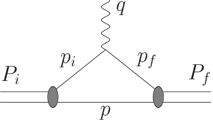
Figure 1: Representation of a virtual photon absorption on a two-body system with the kinematical definitions.

The contribution which we are interested in is shown in Fig. 1. The general expression of the corresponding matrix element between two states with $l=0$, possibly different, is given by

$$\sqrt{2E_{f}\,2E_{i}}\;\left<f|J^{\mu}|i\right>=F_{1}(q^{2})\,(P^{\mu}_{f}+P^{\mu}_{i})+F_{2}(q^{2})\,q^{\mu},$$ (1)

where $q^{\mu}=P^{\mu}_{f}-P^{\mu}_{i}$. Current conservation imposes constraints on the form factors $F_{1}(q^{2})$ and $F_{2}(q^{2})$. For an elastic process, $F_{2}(q^{2})$ has to vanish but this result automatically stems from symmetry arguments alone. It does not imply that current conservation holds at the operator level, as it should. For an inelastic process, the following relationship has to be fulfilled:

$$F_{1}(q^{2})\,(M^{2}_{f}-M^{2}_{i})+F_{2}(q^{2})\,q^{2}=0.$$ (2)

Form factors using the Bethe-Salpeter amplitudes.
For the model under consideration here, the general (and exact) expression of the matrix element of the current, which reduces to a single-particle one in this case, can be written in terms of the Bethe-Salpeter amplitudes, $\chi\raisebox{-4.30554pt}[0.0pt]{\scriptsize{$P$}}(p)$,

$$\sqrt{2E_{f}\,2E_{i}}\;\left<f|J^{\mu}|i\right>=\hskip 270.30118pt$$

$$i\int\frac{d^{4}p}{(2\pi)^{4}}\;\chi\raisebox{-4.30554pt}[0.0pt]{\scriptsize{$P_{f}$}}\Big{(}\frac{1}{2}P_{f}-p\Big{)}\;\left(P^{\mu}_{f}+P^{\mu}_{i}-2\,p^{\mu}\right)\,(p^{2}-m^{2})\;\chi\raisebox{-4.30554pt}[0.0pt]{\scriptsize{$P_{i}$}}\Big{(}\frac{1}{2}P_{i}-p\Big{)}.$$ (3)

For the Wick-Cutkosky model, the Bethe-Salpeter amplitudes take the form of a relatively simple integral representation, i.e. for the lowest energy state with a given orbital angular momentum $l$:

$$\chi\raisebox{-4.30554pt}[0.0pt]{\scriptsize{$P$}}(p)=\int_{-1}^{1}dz\;\frac{g_{n}(z)\;Y_{l}^{m}(\hat{p})\;|\vec{p}\,|^{l}}{(m^{2}-\frac{1}{4}P^{2}-p^{2}-z\,P\cdot p-i\epsilon)^{n+2}},$$ (4)

with $n=l+1$. In this expression, $g_{n}(z)$ is the solution of a second order differential equation [1, 2], that can be solved easily.

Form factors in the non-relativistic limit.
Opposite to the full relativistic calculation, a non-relativistic one can be performed. Using wave functions that are solutions of a Schrödinger equation, general expressions for both elastic and inelastic form factors can be obtained:

$$F_{1}(q^{2})=\int\frac{d\vec{p}}{(2\pi)^{3}}\;\;\phi_{f}\Big{(}\vec{p}-\frac{1}{4}\vec{q}\,\Big{)}\;\;\phi_{i}\Big{(}\vec{p}+\frac{1}{4}\vec{q}\,\Big{)},\hskip 22.76219pt$$

$$F_{2}(q^{2})\,\frac{\vec{q}}{4m}=-\int\frac{d\vec{p}}{(2\pi)^{3}}\;\;\phi_{f}\Big{(}\vec{p}-\frac{1}{4}\vec{q}\,\Big{)}\;\;\frac{\vec{p}}{m}\;\;\phi_{i}\Big{(}\vec{p}+\frac{1}{4}\vec{q}\,\Big{)}.$$ (5)

It can be checked that the above form factors verify the current conservation condition, Eq. (2), provided the interaction is local. The second form factor vanishes in the elastic case.

Form factors in the point-form approach.
It has been shown [7] that a calculation of form factors in the point form approach could be performed relatively easily by using standard wave functions obtained from a mass operator of the form

$$M=M_{free}+M_{int}.$$ (6)

This includes a large class of wave functions, since the sum of the kinetic and potential energies appearing in the standard Schrödinger equation can be identified with the operator $M^{2}$ (up to a factor). This holds for a two-body system and provided the energy $E$ is appropriately redefined. Therefore, wave functions entering the non-relativistic expressions of Eq. (5) can be used. How the matrix element of the single-particle current is calculated has been described in ref. [8]. Instead of using an expression where appropriate boosts have to be performed, we here give one whose Lorentz-covariance is explicit:

$$\sqrt{2E_{f}\,2E_{i}}\;\left<f|J^{\mu}|i\right>=\sqrt{2M_{f}\,2M_{i}}\frac{1}{(2\pi)^{3}}\hskip 170.71652pt$$

$$\times\int d^{4}p\,d^{4}p_{f}\,d^{4}p_{i}\,d\eta_{f}\,d\eta_{i}\;\delta(p^{2}-m^{2})\;\delta(p^{2}_{f}-m^{2})\;\delta(p^{2}_{i}-m^{2})\hskip 42.67912pt$$

$$\times\theta(\lambda_{f}\cdot p_{f})\;\theta(\lambda_{f}\cdot p)\;\theta(\lambda_{i}\cdot p)\;\theta(\lambda_{i}\cdot p_{i})\;\delta^{4}(p_{f}+p-\lambda_{f}\eta_{f})\;\delta^{4}(p_{i}+p-\lambda_{i}\eta_{i})$$

$$\times\phi_{f}\Big{(}(\frac{p_{f}-p}{2})^{2}\Big{)}\;\phi_{i}\Big{(}(\frac{p_{i}-p}{2})^{2}\Big{)}\;\sqrt{(p_{f}+p)^{2}\,(p_{i}+p)^{2}}\;\;\;(p_{f}^{\mu}+p_{i}^{\mu}).$$ (7)

In this expression, all quantities are Lorentz-invariant ones (except obviously for the current which behaves as a 4-vector). The auxiliary variables, $\eta_{i}$ and $\eta_{f}$, have been introduced to make the covariance manifest. When these variables are integrated over, they give rise to 3-dimensional $\delta(...)$-functions

$$\delta\Big{(}\vec{p}_{i}+\vec{p}-\frac{\vec{\lambda}_{i}}{\lambda_{i}^{0}}(p^{0}_{i}+p^{0})\Big{)}\;\;{\rm and}\;\;\delta\Big{(}\vec{p}_{f}+\vec{p}-\frac{\vec{\lambda}_{f}}{\lambda_{f}^{0}}(p^{0}_{f}+p^{0})\Big{)},$$

that are essential relations in the point-form approach. The $\lambda^{\mu}_{i}\;{\rm and}\;\lambda^{\mu}_{f}$ 4-vectors are unit vectors proportional to the 4-momenta of the total system in the initial and final states, $\lambda^{\mu}_{i}=\frac{P^{\mu}_{i}}{M_{i}}\;{\rm and}\;\lambda^{\mu}_{f}=\frac{P^{\mu}_{f}}{M_{f}}$. They can be expressed in terms of the corresponding velocities, $\lambda^{0}=(\sqrt{1-v^{2}}\,)^{\,-1}$ and $\vec{\lambda}=\vec{v}\,(\sqrt{1-v^{2}}\,)^{\,-1}$ (c=1). In the c.m., it can be checked that the wave function $\phi(...)$ only depends on the relative momentum of the two particles. On the other hand, it can also be verified, by direct integration or after performing a change of variable, that the current of the system under consideration is given by $(\,\left<J^{0}\right>\,,\,\vec{\left<J\,\right>\,})=(\,1\,,\,\vec{v}\,)$, in agreement with the standard normalisation of the wave function

$$\int\frac{d\vec{p}}{(2\pi)^{3}}\;\phi^{2}(\vec{p}\,)=1.$$

Expressions of the form factors, $F_{1}(q^{2})$ and $F_{2}(q^{2})$, can be obtained in any frame. With an appropriate change of variables, they can always be expressed in the forms they take in the Breit frame (here defined by $\vec{v}=\vec{v}_{f}=-\vec{v}_{i}$), where they may be simpler. Using auxiliary quantities, $\tilde{F}_{1}(q^{2})$ and $\tilde{F}_{2}(q^{2})$, they read:

$$F_{1}(q^{2})\;\sqrt{2M_{f}\,2M_{i}}=\tilde{F}_{1}(q^{2})\,(M_{f}+M_{i})-\tilde{F}_{2}(q^{2})\,(M_{f}-M_{i}),$$

$$F_{2}(q^{2})\;\sqrt{2M_{f}\,2M_{i}}=-\tilde{F}_{1}(q^{2})\,(M_{f}-M_{i})+\tilde{F}_{2}(q^{2})\,(M_{f}+M_{i}),$$ (8)

with

$$\tilde{F}_{1}(q^{2})=\frac{1+v^{2}}{\sqrt{1-v^{2}}}\int\frac{d\vec{p}}{(2\pi)^{3}}\;\phi_{f}(\vec{p}_{tf})\;\phi_{i}(\vec{p}_{ti}),$$

$$\tilde{F}_{2}(q^{2})\;\vec{v}=-\frac{1+v^{2}}{\sqrt{1-v^{2}}}\int\frac{d\vec{p}}{(2\pi)^{3}}\;\phi_{f}(\vec{p}_{tf})\;\;\frac{\vec{p}}{e_{p}}\;\;\phi_{i}(\vec{p}_{ti}).$$ (9)

In the above equations, the velocity $\vec{v}$, defined in the Breit frame, is related to the momentum transfer by the relation $v^{2}=\frac{Q^{2}+(M_{f}-M_{i})^{2}}{Q^{2}+(M_{f}+M_{i})^{2}}$. The (Lorentz-) transformed momenta are defined as: $(p^{x},p^{y},p^{z})_{tf}=(p^{x},p^{y},\frac{p^{z}-v\,e_{p}}{\sqrt{1-v^{2}}})$ and $(p^{x},p^{y},p^{z})_{ti}=(p^{x},p^{y},\frac{p^{z}+v\,e_{p}}{\sqrt{1-v^{2}}})$, together with $e_{p}=\sqrt{m^{2}+\vec{p}^{\,2}}$.

Wave functions and analytical results.
For the wave functions of the ground and first excited states, $\phi(\vec{p}\,)$ and $\phi^{*}(\vec{p}\,)$, we use solutions obtained with a Coulomb-like potential,

$$\phi(\vec{p}\,)=\sqrt{4\,\pi}\frac{4\,\kappa^{5/2}}{(\kappa^{2}+\vec{p}^{\,2})^{2}},\hskip 28.45274pt$$

$$\phi^{*}(\vec{p}\,)=\sqrt{4\pi}\frac{8\,\kappa^{*5/2}}{(\kappa^{*2}+\vec{p}^{\,2})^{3}}(\kappa^{*2}-\vec{p}^{\,2}),$$ (10)

where $\kappa^{2}=m^{2}-\frac{1}{4}M^{2}$, the total mass $M$ being that one obtained from the Bethe-Salpeter equation for the ground state. It has been shown [11] that the spectrum of the normal states for the Wick-Cutkosky model, which has the same degeneracy as the Coulomb potential, could be reproduced with a 3-dimensional equation and an effective interaction of the Coulomb-type. Due to the appearance of $M^{2}$ in such an equation, the energy redefinition mentioned previously is not even needed in the present case. The wave functions of Eqs. (10) should therefore be a good zeroth order approximation for our study, including the extreme case $M^{2}=0$. Accordingly, we assume $\kappa^{*2}=0.25\,\kappa^{2}=0.25\,(m\alpha_{eff}/2)^{2}$, which differs from the Bethe-Salpeter result, $\kappa^{*2}=m^{2}-\frac{1}{4}M^{*2}$, by a few percent. With these wave functions, the form factors can be calculated analytically. We checked that the main features evidenced by our results were insensitive to this choice by using a different (numerical) wave function [10], more in the spirit of the point-form approach, i.e. obtained directly from the linear mass operator, Eq. (6).

In the non-relativistic case, the elastic and inelastic form factors are respectively given by:

$$F_{1}(q^{2})=\frac{\kappa^{4}}{(\kappa^{2}+Q^{2}/16)^{2}},\;\;\;\;\;\;F_{2}(q^{2})=0,\hskip 56.9055pt$$

$$F_{1}(q^{2})=-\sqrt{2}\,\frac{64\,\kappa^{4}\,Q^{2}}{(9\kappa^{2}+Q^{2})^{3}},\;\;\;\;\;\;F_{2}(q^{2})=-\sqrt{2}\,\frac{192\,\kappa^{6}}{(9\kappa^{2}+Q^{2})^{3}}.$$ (11)

Taking into account that $M^{2}_{f}-M^{2}_{i}=3\,\kappa^{2}$, one can verify that the condition of current conservation, Eq. (2), is fulfilled.

In the point-form approach, the elastic form factor, written in a way that resembles the non-relativistic one, reads:

$$F_{1}(q^{2}=-Q^{2})=\frac{\kappa^{4}\,\left(1+2\frac{Q^{2}}{4M^{2}}\right)}{\Big{(}\kappa^{2}+\frac{Q^{2}}{16\,\big{(}1+\frac{Q^{2}}{4M^{2}}\big{)}}\Big{)}^{2}\;\left(1+\frac{Q^{2}}{4M^{2}}\right)^{4}},\;\;\;\;\;\;F_{2}(q^{2}=-Q^{2})=0.$$ (12)

Interestingly, the factor $1/(1+\frac{Q^{2}}{4M^{2}})$ which multiplies the quantity $\frac{Q^{2}}{16}$ in the denominator of $F_{1}(q^{2})$ is the same as the one sometimes introduced by hand in order to account for the Lorentz-contraction effect (see discussion in ref. [12]). Contradicting asymptotic results (in QCD for instance), the range of validity of this recipe is limited to small $Q^{2}$. Curiously, part of the extra factors also look like a Lorentz-contraction effect.

As for the inelastic form factors for a transition from the ground- to the first radially excited state, they are most easily expressed in terms of the quantities, $\tilde{F}_{1}(q^{2})$ and $\tilde{F}_{2}(q^{2})$, which can also be calculated analytically:

$$\tilde{F}_{1}(q^{2})=-\sqrt{2}\,\frac{64\,\kappa^{4}\,v^{2}\,(16\,m^{2}-4\kappa^{2}(1-v^{2}))}{(9\kappa^{2}+v^{2}\,(16\,m^{2}-10\kappa^{2})+v^{4}\kappa^{2})^{3}}\,(1+v^{2})\,(1-v^{2})^{3},$$

$$\tilde{F}_{2}(q^{2})=-\sqrt{2}\,\frac{64\,(3+v^{2})\,\kappa^{6}}{(9\kappa^{2}+v^{2}\,(16\,m^{2}-10\kappa^{2})+v^{4}\kappa^{2})^{3}}\,(1+v^{2})\,(1-v^{2})^{4},$$ (13)

where $v^{2}$ is defined after Eq. (9). These expressions generalise those for the non-relativistic case, Eq. (11) (it is reminded that in this limit $Q^{2}=16\,v^{2}\,m^{2}$). In contrast however, they do not allow us to fulfil current conservation, Eq. (2).

3 Results

Table 1: Elastic form factor, $F_{1}(q^{2})$, for the ground-state. Units for $E$ and $\kappa$ are the constituent mass, $m$. Results are presented for different couplings and, for each of them, for different approaches: Bethe-Salpeter equation ($B.S.$), non-relativistic calculation ($N.R.$) and point-form approach ($P.F.$). The value of $\alpha$ referred to in the table corresponds to the Bethe-Salpeter equation while the coupling for the “non-relativistic” model, $\alpha_{eff}$, is chosen in such a way to reproduce the binding energy for the ground state.

$Q^{2}/m^{2}$	0.01	0.1	1.0	10.0
$\alpha=1$
$E=0.0842,\kappa^{2}=0.0824$
$B.S.$	0.984	0.856	0.309	0.137-01
$N.R.$	0.985	0.864	0.323	0.135-01
$P.F.$	0.984	0.853	0.298	0.097-01
$\alpha=3$
$E=0.432,\kappa^{2}=0.385$
$B.S.$	0.996	0.962	0.705	0.139
$N.R.$	0.996	0.968	0.740	0.145
$P.F.$	0.994	0.948	0.620	0.056
$\alpha=2\pi$
$E=2.0,\kappa^{2}=1.0$
$B.S.$	0.998	0.983	0.848	0.339
$N.R.$	0.997	0.987	0.884	0.378
$P.F.\,(E=1.90)$	0.613	0.397-01	0.110-03	0.124-06
$P.F.\,(E=1.95)$	0.181	0.142-02	0.191-05	0.196-08

In Table 1, results are presented for elastic form factors corresponding to small ($\alpha=1$), moderate ($\alpha=3$) and strong binding ($\alpha=2\pi$). In the last case, the elastic form factors in the point form vanish at finite $Q^{2}$ and results are actually those obtained when approaching the limit $\alpha\rightarrow 2\pi$, with $E=1.90\,m$ and $E=1.95\,m$. For these energy values, the non-relativistic results, to which the previous ones may be compared, are essentially the same as for $E=2.0\,m$, given in the table.

One immediately notices that the non-relativistic results are very close to the exact ones for all cases, including the extreme case where the total mass of the system is zero. This agreement extends up to $Q^{2}=100\,m^{2}$ with an error of 20% for $\alpha=1$ and 50% for $\alpha=2\,\pi$. The discrepancy at small momentum transfers is typically of the order of $\frac{Q^{2}}{16m^{2}}$. Most probably, it can be traced back to the wave function used in the non-relativistic calculation or to the electromagnetic single-particle current. These ingredients do not fully account for corrections due to factors $\frac{m}{e}$ (in the potential for instance) or for the field-theory character of the Wick-Cutkosky model. A major lesson of these results is that relativistic effects are not necessarily important and that most probably, for any non-relativistic calculation of form factors, there exists a covariant calculation (the exact one in the present case) which gives very close results over a large range of momentum transfers. However, this does not mean that this calculation involves all relativistic effects and is physically relevant, especially with respect to current conservation. An example is provided by the deuteron electro-disintegration near threshold in the light-front approach. Two covariant calculations of the transition form factors have been shown to be very close to the non-relativistic ones up to $Q^{2}=10$ (GeV/c)² [13], completely missing the contribution due to the pair term whose relativistic character is well known. In the non-relativistic approach, this contribution, which is required to fulfil current conservation, is essential to account for experiment in the low momentum transfer range. How this contribution appears in the covariant light-front formalism was shown later on [14].

The comparison with the point-form results evidences a discrepancy that increases with the momentum transfer as well as with the coupling strength. It becomes especially large when approaching the extreme case where $M=0$. Two features are worthwhile to be mentioned, that stem from examining the analytic expressions of the form factors, Eq. (12). First, there is a contribution to the squared-charge radius which varies like $\frac{1}{M^{2}}$, as it was found numerically in ref. [9]. Second, the form factor drops more quickly with $Q^{2}$ than in the exact or in the non-relativistic calculations, roughly like $\frac{1}{Q^{6}}$ instead of $\frac{1}{Q^{4}}$. This can be seen in Table 1 for $E=1.90\,m$ and $E=1.95\,m$ and is in agreement with what the examination of the Born amplitude reveals. The effect becomes especially sizeable when approaching $Q^{2}=4\,M^{2}$ and beyond.

Table 2: Inelastic form factors, $F_{1}(q^{2})\;{\rm and}\;F_{2}(q^{2})$, for a $l=0\rightarrow l=0^{*}$ transition, and $\alpha=3,E_{i}=0.4322\,m,\kappa_{i}^{2}=0.385\,m^{2},E_{f}=0.1036\,m,\kappa_{f}^{2}=0.101\,m^{2}$ for the exact calculation and $0.096\,m^{2}$ for the non-relativistic one.

$Q^{2}/m^{2}$	0.01	0.1	1.0	10.0
$B.S.$
$F_{1}$	-0.032-01	-0.298-01	-0.145-00	-0.584-01
$F_{2}$	-0.369-00	-0.340-00	-0.165-00	-0.665-02
$N.R.$
$F_{1}$	-0.032-01	-0.296-01	-0.151-00	-0.550-01
$F_{2}$	-0.369-00	-0.342-00	-0.174-00	-0.636-02
$P.F.$
$F_{1}$	-0.101-01	-0.372-01	-0.140-00	-0.283-01
$F_{2}$	-0.324-00	-0.293-00	-0.119-00	-0.022-02

Results for an inelastic transition are given in Table 2. The results obtained in the non-relativistic approach compare well with the exact ones over the full range of $Q^{2}$. The slight discrepancies are quite similar to those observed for the elastic form factors. While the point-form results compare well with the other ones in the intermediate range, $0.1<Q^{2}/m^{2}<3$, they fail at low and at large $Q^{2}$. In the former case, $F_{1}(q^{2})$ does not go to zero when $Q^{2}\rightarrow 0$, violating the current conservation, Eq. (2). In the latter case, $F_{2}(q^{2})$ evidences a change in sign around $Q^{2}\simeq 10\,m^{2}$, also preventing one from fulfilling this relation. This can be traced back to the different behaviour of the intermediate form factors $\tilde{F}_{1}$ and $\tilde{F}_{2}$, which keep the same sign but scale like $Q^{-6}$ and $Q^{-8}$ at high $Q^{2}$, respectively. These results for an inelastic transition complement those for the elastic case. Again, a large discrepancy with exact results appears, but the bad behaviour of form factors at low as well as large momentum transfers is more clearly correlated with a violation of current conservation.

4 Discussion and conclusion

The present study was motivated by the necessity to check the reliability of retaining the single-particle current for the calculation of form factors in the point form of quantum relativistic mechanics, which was recently employed in different works [8, 9]. With this aim, we considered a simple model where the exact result is known. It was found that the non-relativistic approach does particularly well up to momentum transfers of 3-4 times the constituent mass, including the case of a strong binding. While the point-form approach does correctly for small bindings and small couplings, large discrepancies with the exact results appear as soon as the momentum transfer or the coupling increases. Detailed examination evidences three features.
- The form factors decrease more rapidly than they should. This points to an extra $\frac{1}{Q^{2}}$ dependence that is absent in the exact calculation.
- For strong couplings, corresponding to a sizeable presence of high momentum components in the wave function, the charge radius turns out to be much larger than the exact one.
- Finally, as emphasised by the results for an inelastic transition, current conservation is strongly violated.

Although it is not quite certain, there is good reason to believe that the non-relativistic calculation does relatively well because it fulfils current conservation. With this respect, the failure of the point-form approach is likely to reside in the incomplete character of the current operator. Current conservation may be enforced by the replacement

$$\left<J^{\mu}\right>\;\;\rightarrow\;\;\left<J^{\mu}\right>-q^{\mu}\left<J_{\nu}\right>\cdot\,q^{\nu}/q^{2}.$$

Apart from the unsatisfactory character of this recipe, due to the presence of a pole at $q^{2}=0$ , it does not solve the problem of the too fast drop-off of the elastic charge form factor at high $Q^{2}$. Most probably, two-body currents have to be considered. This is consistent with the known fact that, in the point form approach, the interaction appears in all the components of the 4-momentum operator [15]. Whether a minimal set of two-body currents will be sufficient to provide results in better agreement with the exact ones is not clear however. These currents should also correct for the failure of the point-form results to reproduce the Born amplitude expected from the underlying field-theory model.

The above results cannot be applied directly to the calculation of the deuteron or nucleon form factors [8, 9]. However, the qualitative similarity in the results strongly suggests that the kinematical boost, which provided a nice description of the nucleon form factors, represents an incomplete account of relativistic effects. More likely, the agreement is the consequence of neglecting significant contributions to the current. This conclusion is to be preferred with two respects.
- It leaves some room for the well known contribution of the coupling of the nucleon to the photon through vector-meson exchange (vector-meson dominance mechanism), which roughly provides half of the proton’s squared charge radius.
- On the other hand, it leaves room for another relativistic effect related to the nature of the coupling of the constituents to the exchanged boson. This effect increases the form factor at high $Q^{2}$ rather than the opposite as in ref. [9]. It is known to explain the different asymptotic form factors in a non-relativistic and a relativistic calculation in QCD, which scale like $\frac{1}{Q^{8}}$ and $\frac{1}{Q^{4}}$, respectively (see for instance refs. [16, 17]).

Altogether, two-body currents should produce quite sizeable contributions. Their role seems to be more essential in the point form than in other approaches.

Acknowledgements We are very indebted to W. Klink for information about his work, which largely motivated the present one. Helpful discussions with him are greatly appreciated.

References

- [1] G.C. Wick, Phys. Rev. 96 (1954) 1124.
- [2] R.E. Cutkosky, Phys. Rev. 96 (1954) 1135.
- [3] E.E. Salpeter and H.A. Bethe, Phys. Rev. 84 (1951) 1232.
- [4] B. Desplanques, R. Medrano, S. Noguera and L. Theußl: contribution to the XVIIth European Conference on Few-Body Problems in Physics, 11-16 September 2000, Évora, Portugal.
- [5] V.A. Karmanov and A. Smirnov, Nucl. Phys. A 575 (1994) 520.
- [6] P.A.M. Dirac, Rev. Mod. Phys. 21 (1949) 392.
- [7] W.H. Klink, Phys. Rev. C 58 (1998) 3587.
- [8] T.W. Allen, W.H. Klink and W.N. Polyzou, nucl-th/0005050.
- [9] R. Wagenbrunn, S. Boffi, W.H. Klink, W. Plessas and M. Radici, nucl-th/0010048.
- [10] B. Desplanques and L. Theußl, in preparation.
-
[11]
A. Amghar and B. Desplanques, Few-Body Syst. 28 (2000) 65;
A. Amghar, B. Desplanques and L. Theußl, nucl-th/0012051. - [12] J.L. Friar, Ann. Phys. 81 (1973) 332; Nucl. Phys. A 264 (1976) 455.
-
[13]
B.D. Keister, Phys. Rev. C 37 (1988) 1765;
A. Amghar, B. Desplanques and V.A. Karmanov, Nucl. Phys. A 567 (1994) 919. - [14] B. Desplanques, V.A. Karmanov and J.F. Mathiot, Nucl. Phys. A 589 (1995) 697.
- [15] W.H. Klink, nucl-th/0012033.
- [16] C. Alabiso and G. Schierholz, Phys. Rev. D 10 (1974) 960.
- [17] B. Desplanques et al., Few-Body Syst. 29 (2000) 169.