Improved lower bounds for the ground-state energy of many-body systems

Abstract

New lower bounds for the binding energy of a quantum-mechanical system of interacting particles are presented. The new bounds are expressed in terms of two-particle quantities and improve the conventional bounds of the Hall-Post type. They are constructed by considering not only the energy in the two-particle system, but also the structure of the pair wave function. We apply the formal results to various numerical examples, and show that in some cases dramatic improvement over the existing bounds is reached.

I Introduction

One of the central problems in quantum many-body physics is to find the energy of a system of $A$ particles interacting with given two-body potentials. Variational techniques yield an upper bound to the exact energy. The determination of a strict lower bound can then provide a natural and useful complement.

In recent years there has been renewed interest in deriving such lower bounds, mostly in connection with quark models in hadron spectroscopy [1], or the limits for Borromean phenomena in loosely bound systems [2, 3, 4, 5]. Earlier uses of lower bounds were focussed on thermodynamical considerations [6], or the problem of stability in self-gravitating systems [7, 8].

Up to now all lower bounds are based on the Hall-Post decomposition [9, 10] of the hamiltonian into two-body clusters, and subsequent application of the variational principle in two-body space. Several variants and extensions have been proposed, e.g. an optimal decomposition in case of three [11] or four [12] unequal masses. The case of identical fermions was recently studied in [13].

In its most useful form, a lower bound of the Hall-Post type is expressed in terms of the ground-state energy in a two-body system. Finding this two-body energy usually goes together with determining the wave function of the ground-state pair. We show in this paper that by using the structure of the pair wave function one can always improve the Hall-Post bound, and that the improvement is sometimes spectacular. Our results apply to boson and fermion systems, both with and without the presence of an external potential, and irrespective of the local or nonlocal character of the two-body potentials. We do restrict ourselves to systems of identical particles, leaving a study of the unequal mass case for future work.

Loosely speaking, the Hall-Post bound implies that the ground state for $A$ identical particles is a superposition of $\frac{1}{2}A(A-1)$ pairs in the lowest-energy state of a modified hamiltonian. However, because of the correlated structure of such a pair, it is in general not possible to reach a pair occupation of $\frac{1}{2}A(A-1)$, except in the case of noninteracting bosons. For any given pair, there exists a maximal value for the occupancy that can be reached in an $A$-body state. The remainder of the $\frac{1}{2}A(A-1)$ pairs must then necessarily be in a state with higher energy. This allows the construction of a new lower bound, whose value is increased with respect to the Hall-Post case.

The present paper is organized as follows. In Section II we first establish notations, introduce cluster decompositions of the many-body hamiltonian, and rederive the Hall-Post inequalities. Next we point out in Section III how the Hall-Post bound can be improved in the case of fixed-center bosonic systems. The equivalent case for fermions is treated in Section IV. The modifications that enter when considering self-bound (translationally invariant) systems are discussed in Section V. Finally, we apply the formal results to various numerical examples, which are collected in Section VI. Section VII contains a global summary and points out some remaining problems.

II General remarks on cluster decompositions of the hamiltonian for a system of identical particles

A Notational conventions

We restrict ourselves to systems of identical particles and follow the notational conventions of [14]. In particular, single-particle coordinates are generically written as $x_{1},x_{2},\dots$, and should be regarded as spatial coordinates in $d$ dimensions. Spin or isospin degrees of freedom are not explicitly mentioned, but may be assumed to be included in the $x_{i}$ dependence of the wave functions and operators.

For a system of $A$ particles we consider a hamiltonian $\hat{H}_{A}[\alpha]$ which is a sum of one-body and two-body operators with variable relative weight,

$$\hat{H}_{A}[\alpha](x_{1},\dots,x_{A})=\alpha\sum_{i_{1}=1,\dots,A}t(x_{i_{1}})+\sum_{i_{1}<i_{2}=1,\dots,A}v(x_{i_{1}},x_{i_{2}}).$$ (1)

Using a combinatorial identity we can rewrite $\hat{H}_{A}[\alpha=1]$, for any $N$ with $2\leq N\leq A$, as

$$\hat{H}_{A}[1](x_{1},\dots,x_{A})=\frac{1}{\left(\begin{array}[]{c}A-2\\ N-2\end{array}\right)}\sum_{i_{1}<\dots<i_{N}=1,\dots,A}\hat{H}_{N}[\frac{N-1}{A-1}](x_{i_{1}},\dots,x_{i_{N}}).$$ (2)

The hamiltonian $\hat{H_{N}}[\frac{N-1}{A-1}]$ for clusters of $N$ particles is related to the original hamiltonian $\hat{H_{A}}[1]$ for $A$ particles, but has different relative weights for its one-body and two-body components (or, equivalently: a different coupling strength of the two-body interaction). We can now make the weights equal again by absorbing the difference in an additional one-body term. As shown in Section II B, this leads to sumrules for the energy which are generalizations of the well-known Koltun sumrule [16]. Alternatively, we can keep the different coupling strength in the $N$-particle hamiltonian. This will lead to another set of sumrules, derived in Section II C, from which the Hall-Post inequalities immediately follow.

One of the ingredients in these sumrules are the spectroscopic factors related to the removal of particles from the $A$-particle system in its ground state. These are defined as follows.

The $A$-particle ground state $\Psi_{0(A)}[1]$ of $\hat{H}_{A}[1]$ can always be expanded in terms of the complete orthonormal set of $N$-particle eigenstates $\Psi_{\nu(N)}[\alpha]$ of $\hat{H}_{N}[\alpha]$,

$$\Psi_{0(A)}[1](x_{1},\dots,x_{A})={\left(\begin{array}[]{c}A\\ N\end{array}\right)}^{-1/2}\sum_{\nu(N)}\Psi_{\nu(N)}[\alpha](x_{1},\dots,x_{N})\psi_{\nu(N)}[\alpha](x_{N+1},\dots,x_{A}).$$ (3)

The expansion coefficients $\psi_{\nu(N)}[\alpha]$ are the overlap functions between the $\Psi_{\nu(N)}[\alpha]$ and $\Psi_{0(A)}[1]$,

$$\psi_{\nu(N)}[\alpha](x_{N+1},\dots,x_{A})=$$ (7)

$${\left(\begin{array}[]{c}A\\ N\end{array}\right)}^{1/2}\int dx_{1}\dots dx_{N}\Psi^{*}_{\nu(N)}[\alpha](x_{1},\dots,x_{N})\Psi_{0(A)}[1](x_{1},\dots,x_{A}),$$

and their normalization yields the corresponding spectroscopic factor $S_{\nu(N)}[\alpha]$,

$$S_{\nu(N)}[\alpha]=\int dx_{N+1}\dots dx_{A}|\psi_{\nu(N)}[\alpha](x_{N+1},\dots,x_{A})|^{2},$$ (8)

that is, the squared amplitude for removing $A-N$ particles from $\Psi_{0(A)}[1]$ and ending up in $\Psi_{\nu(N)}[\alpha]$.

Obviously, the spectroscopic factors are positive, and the completeness of the set $\Psi_{\nu(N)}[\alpha]$ implies the sumrule

$$\sum_{\nu(N)}S_{\nu(N)}[\alpha]={\left(\begin{array}[]{c}A\\ N\end{array}\right)}.$$ (9)

Note that the $S_{\nu(N)}[\alpha]$ can also be interpreted as the occupation number of the state $\Psi_{\nu(N)}[\alpha]$ in the ground state $\Psi_{0(A)}[1]$, since Eq.(8) can be rewritten as

$$S_{\nu(N)}[\alpha] = \int dx_{1}\dots dx_{N}dx^{\prime}_{1}\dots dx^{\prime}_{N}\Psi_{\nu(N)}^{*}[\alpha](x_{1},\dots,x_{N})\rho^{(N)}(x_{1},\dots,x_{N};x^{\prime}_{1},\dots,x^{\prime}_{N})$$ (11)

$$\Psi_{\nu(N)}[\alpha](x^{\prime}_{1},\dots,x^{\prime}_{N}),$$

in terms of the $N$-body density matrix

$$\rho^{(N)}(x_{A-N+1},\dots,x_{A};x^{\prime}_{A-N+1},\dots,x^{\prime}_{A})={\left(\begin{array}[]{c}A\\ N\end{array}\right)}\int dx_{1}\dots dx_{A-N}$$ (14)

$$\Psi_{0(A)}^{*}[1](x_{1},\dots,x_{A-N},x^{\prime}_{A-N+1},\dots,x^{\prime}_{A})\Psi_{0(A)}[1](x_{1},\dots,x_{A-N},x_{A-N+1},\dots,x_{A}).$$ (15)

The above equations hold for fixed-center systems, in which the one-body part of the hamiltonian contains an external potential. For self-bound systems the one-body part is purely kinetic, and the two-body part depends on relative coordinates only, i.e. $v(x_{1},x_{2})\equiv v(x_{1}-x_{2})$. Since the intrinsic eigenstates of the hamiltonian are translationally invariant, some modifications [14] are needed.

The intrinsic kinetic energy is obtained by subtracting the center-of-mass from the total kinetic energy,

$$\hat{T^{\prime}}_{A}=-\frac{1}{2m}\sum_{i_{1}=1,\dots,A}\partial^{2}_{i_{1}}+\frac{1}{2Am}(\sum_{i_{1}=1,\dots,A}\partial_{i_{1}})^{2}=-\frac{1}{2Am}\sum_{i_{1}\leq i_{2}=1,\dots,A}(\partial_{i_{1}}-\partial_{i_{2}})^{2},$$ (16)

and is seen to behave as a two-body operator with an $A$-dependent coupling strength. Defining the intrinsic hamiltonian with variable coupling strength as

$$\hat{H^{\prime}}_{A}[\alpha]=\alpha\hat{T^{\prime}}_{A}++\sum_{i_{1}<i_{2}=1,\dots,A}v(x_{i_{1}}-x_{i_{2}}),$$ (17)

the decomposition (2) gets modified to

$$\hat{H^{\prime}}_{A}[1](x_{1},\dots,x_{A})=\frac{1}{\left(\begin{array}[]{c}A-2\\ N-2\end{array}\right)}\sum_{i_{1}<\dots<i_{N}=1,\dots,A}\hat{H^{\prime}}_{N}[\frac{N}{A}](x_{i_{1}},\dots,x_{i_{N}}).$$ (18)

The $A$-particle ground-state wave function can be expanded in a complete orthonormal set of intrinsic $N$-particle eigenstates [14], the self-bound equivalent of Eq.(3) being

$$\Psi_{0(A)}[1](x_{1},\dots,x_{A}) = {\left(\begin{array}[]{c}A\\ N\end{array}\right)}^{-1/2}\sum_{\nu(N)}\Psi_{\nu(N)}[\alpha](x_{1},\dots,x_{N})$$ (22)

$$\times\psi_{\nu(N)}[\alpha](x_{N+1}-R_{N},\dots,x_{A}-R_{N}),$$

where $R_{N}=\frac{1}{N}\sum_{i=1}^{N}x_{i}$; the overlap functions are defined as

$$\psi_{\nu(N)}[\alpha](x_{N+1},\dots,x_{A}) = {\left(\begin{array}[]{c}A\\ N\end{array}\right)}^{1/2}\int dx_{1}\dots dx_{N}\delta(R_{N})\Psi^{*}_{\nu(N)}[\alpha](x_{1},\dots,x_{N})$$ (26)

$$\times\Psi_{0(A)}[1](x_{1},\dots,x_{A}),$$

whereas Eqs.(8,9) remain unchanged.

The spectroscopic factor $S_{\nu(N)}$, as defined by Eq.(8), can again be viewed as the occupation number of the intrinsic $N$-particle state $\Psi_{\nu(N)}$ in the $A$-particle ground state, but this occupation number now also includes a summation over all possible states of $N$-particle center-of-mass motion, i.e. using

$$\int dK\frac{\exp{(-iKR_{N})}}{(2\pi)^{d/2}}\frac{\exp{(iKR^{\prime}_{N})}}{(2\pi)^{d/2}}=\delta(R_{N}-R^{\prime}_{N}),$$ (27)

we can express the spectroscopic factor as

$$S_{\nu(N)}[\alpha] = \int dx_{1}\dots dx_{N}dx^{\prime}_{1}\dots dx^{\prime}_{N}\delta(R_{N}-R^{\prime}_{N})\Psi_{\nu(N)}^{*}[\alpha](x_{1},\dots,x_{N})$$ (29)

$$\rho^{(N)}(x_{1},\dots,x_{N};x^{\prime}_{1},\dots,x^{\prime}_{N})\Psi_{\nu(N)}[\alpha](x^{\prime}_{1},\dots,x^{\prime}_{N}).$$

The $N$-body density matrix for a self-bound system, defined as

$$\rho^{(N)}(x_{A-N+1},\dots,x_{A};x^{\prime}_{A-N+1},\dots,x^{\prime}_{A})={\left(\begin{array}[]{c}A\\ N\end{array}\right)}\int dx_{1}\dots dx_{A-N}\delta(R_{A-N})$$ (32)

$$\Psi_{0(A)}^{*}[1](x_{1},\dots,x_{A-N},x^{\prime}_{A-N+1},\dots,x^{\prime}_{A})\Psi_{0(A)}[1](x_{1},\dots,x_{A-N},x_{A-N+1},\dots,x_{A}),$$ (33)

is the proper extension of the one-body density matrix for translationally invariant systems in [14, 15].

B Generalized Koltun sumrules

For fixed-center systems the decomposition (2) can be reshuffled so as to have the same hamiltonian in $A$-particle and $N$-particle space, at the expense of an additional one-body term,

$$\hat{H}_{A}[1](x_{1},\dots,x_{A})=\frac{1}{\left(\begin{array}[]{c}A-2\\ N-2\end{array}\right)}\sum_{i_{1}<\dots<i_{N}=1,\dots,A}\hat{H}_{N}[1](x_{i_{1}},\dots,x_{i_{N}})-\frac{A-N}{N-1}\sum_{i_{1}=1,\dots,A}t(x_{i_{1}}).$$ (34)

The expectation value of (34) in the $A$-particle ground state, expanded according to Eq.(3), can be worked out using Eqs.(7,8) and reads

$$E_{0(A)}[1]=\frac{N}{A+N-1}\left\{T_{0(A)}-\frac{1}{\left(\begin{array}[]{c}A-2\\ N-1\end{array}\right)}\sum_{\nu(N)}(E_{\nu(N)}[1]-E_{0(A)}[1])S_{\nu(N)}[1]\right\}.$$ (35)

Here the ground-state energy has been expressed in terms of the expectation value $T_{0(A)}$ of the one-body field and the first energy-weighted moment of the distribution of $(A-N)$-particle removal strength (or mean removal energy). This is a generalization of the familiar Koltun sumrule [16] for $N=A-1$,

$$E_{0(A)}[1]=\frac{1}{2}\left\{T_{0(A)}-\sum_{\nu(A-1)}\left(E_{\nu(A-1)}[1]-E_{0(A)}[1]\right)S_{\nu(A-1)}[1]\right\},$$ (36)

where the distribution of single-particle removal strength is experimentally accessible through single-particle (SP) knock-out reactions [17, 18].

For self-bound systems we can [in analogy to Eq.(34)] restore in Eq.(18) the original hamiltonian at the expense of an additional (intrinsic) kinetic term,

$$\hat{H^{\prime}}_{A}[1](x_{1},\dots,x_{A})=\frac{1}{\left(\begin{array}[]{c}A-2\\ N-2\end{array}\right)}\sum_{i_{1}<\dots<i_{N}=1,\dots,A}\hat{H^{\prime}}_{N}[1](x_{i_{1}},\dots,x_{i_{N}})-\frac{A-N}{N}\hat{T^{\prime}}_{A}.$$ (37)

The ground-state expectation value of Eq.(37), evaluated by means of Eqs.(22,26), then reads

$$E_{0(A)}[1]=\frac{N}{A+N-1}\left\{\frac{N-1}{N}T^{\prime}_{0(A)}-\frac{1}{\left(\begin{array}[]{c}A-2\\ N-1\end{array}\right)}\sum_{\nu(N)}(E_{\nu(N)}[1]-E_{0(A)}[1])S_{\nu(N)}[1]\right\}.$$ (38)

The result for the case of $N=A-1$,

$$E_{0(A)}[1]=\frac{1}{2}\left\{\frac{A-2}{A-1}T^{\prime}_{0(A)}-\sum_{\nu(A-1)}(E_{\nu(A-1)}[1]-E_{0(A)}[1])S_{\nu(A-1)}[1]\right\},$$ (39)

is the Koltun sumrule for self-bound systems (including the correct recoil factor for the kinetic energy [14, 19]).

C Hall-Post inequalities

The expectation value of Eq.(2), with the modified coupling strength in the $N$-particle hamiltonian, can be evaluated in the same way as Eq.(35),

$$E_{0(A)}[1]=\frac{1}{\left(\begin{array}[]{c}A-2\\ N-2\end{array}\right)}\sum_{\nu(N)}E_{\nu(N)}[\frac{N-1}{A-1}]S_{\nu(N)}[\frac{N-1}{A-1}].$$ (40)

This expression forms the basis for deriving the lower bounds considered in the next Section. At the simplest level, combining Eq.(40) with the trivial inequality resulting from the spectroscopic sumrule (9),

$$0\leq S_{\nu(N)}[\frac{N-1}{A-1}]\leq{\left(\begin{array}[]{c}A\\ N\end{array}\right)},$$ (41)

immediately leads to inequalities of the Hall-Post type

$$E_{0(A)}[1]\geq\frac{A(A-1)}{N(N-1)}E_{0(N)}[\frac{N-1}{A-1}].$$ (42)

For self-bound systems the $A$-particle ground-state energy can be likewise evaluated, from the expectation value of Eq.(18), in terms of intrinsic $N$-particle energies and occupation numbers, and reads

$$E_{0(A)}[1]=\frac{1}{\left(\begin{array}[]{c}A-2\\ N-2\end{array}\right)}\sum_{\nu(N)}E_{\nu(N)}[\frac{N}{A}]S_{\nu(N)}[\frac{N}{A}].$$ (43)

The Hall-post inequalities

$$E_{0(A)}[1]\geq\frac{A(A-1)}{N(N-1)}E_{0(N)}[\frac{N}{A}],$$ (44)

then follow immediately from Eq.(41).

III Improved lower bounds for fixed-center bosonic systems

A Derivation of new lower bounds

From now on we concentrate on the most relevant case $N=2$, and try to derive lower bounds for the $A$-particle ground-state energy in terms of two-body quantities. At present, such a lower bound is given by the Hall-Post inequality (42),

$$E_{0(A)}[1]\geq{\left(\begin{array}[]{c}A\\ 2\end{array}\right)}E_{0(2)}[\frac{1}{A-1}],$$ (45)

which is usually derived by applying a variational principle in two-body space [2]. As was shown in Section II C, the Hall-Post inequality is actually an equality when expressed in terms of two-body energies and occupations,

$$E_{0(A)}[1]=\sum_{\nu(2)}E_{\nu(2)}[\frac{1}{A-1}]S_{\nu(2)}[\frac{1}{A-1}].$$ (46)

In order to simplify notations we drop the coupling strength dependence in this Section, as it will be fixed to $\alpha=1$ for $A$-particle and $\alpha=\frac{1}{A-1}$ for two-particle quantities. It is clear from Eqs.(45,46) that in the traditional lower bound the distribution of pair strength $S_{\nu(2)}$ is approximated by concentrating all strength in the two-body ground state, i.e. by the distribution

$$S_{\nu(2)}\approx\delta_{0\nu}{\left(\begin{array}[]{c}A\\ 2\end{array}\right)},$$ (47)

which exhausts the sumrule (9).

This assumption can only be realistic for weakly correlated systems. For a non-interacting Bose system [$v\equiv 0$ in Eq.(1)] it holds exactly. The uncorrelated eigenstates are product-type wave functions,

$$\Psi^{\mbox{unc}}_{0(A)}(x_{1},\dots,x_{A})=\prod_{i=1,\dots,A}\chi(x_{i}),\,\,\,\,\,\Psi^{\mbox{unc}}_{0(2)}(x_{1},x_{2})=\chi(x_{1})\chi(x_{2}),$$ (48)

where $\chi(x)$ is the SP eigenstate of the one-body hamiltonian $t(x)$ corresponding to the lowest energy $\epsilon_{0}$. As a consequence, $S_{0(2)}^{\mbox{unc}}=A(A-1)/2$, and the Hall-Post lower bound coincides with the exact result,

$$E_{0(A)}^{\mbox{unc}}=A\epsilon_{0}={\left(\begin{array}[]{c}A\\ 2\end{array}\right)}\frac{1}{A-1}2\epsilon_{0}={\left(\begin{array}[]{c}A\\ 2\end{array}\right)}E_{0(2)}^{\mbox{unc}}.$$ (49)

For strongly correlated systems we expect that the occupation $S_{0(2)}$ can deviate substantially from $A(A-1)/2$, and the Hall-Post lower bound will be far from the exact result.

In order to improve on this situation we need to take into account correlations in the structure of the many-boson eigenstates. As it is more convenient to work in second quantization, we define $\varphi_{\nu(2)}^{\dagger}$ as the creation operator for the two-body eigenstate $\Psi_{\nu(2)}$, i.e.

$$\mid\Psi_{\nu(2)}\rangle=\varphi^{\dagger}_{\nu(2)}\mid\rangle.$$ (50)

The occupation $S_{\nu(2)}$, as defined by Eq.(8) or Eq.(11), is then simply written as

$$S_{\nu(2)}=\langle\Psi_{0(A)}\mid\varphi^{\dagger}_{\nu(2)}\varphi^{\mbox{}}_{\nu(2)}\mid\Psi_{0(A)}\rangle.$$ (51)

We now consider the upper bound $S_{\nu(2)}^{\mbox{max}}$ for $S_{\nu(2)}$,

$$S_{\nu(2)}^{\mbox{max}}=\max_{\Psi_{A}}\left\{\langle\Psi_{A}\mid\varphi^{\dagger}_{\nu(2)}\varphi^{\mbox{}}_{\nu(2)}\mid\Psi_{A}\rangle\right\},$$ (52)

where the maximum is taken with respect to all normalized $A$-boson eigenstates. This upper bound only requires knowledge of the two-body state $\Psi_{\nu(2)}$; its explicit construction is pointed out in Section III B.

Since $S_{\nu(2)}^{\mbox{max}}$ is better than the trivial upper bound (41), the following inequality holds,

$$S_{\nu(2)}\leq S_{\nu(2)}^{\mbox{max}}\leq{\left(\begin{array}[]{c}A\\ 2\end{array}\right)}.$$ (53)

In combination with Eq.(46) this results in a sequence of new lower bounds ${\cal L}_{\mu}$, with $\mu=0,1,\dots$ , for the ground-state energy,

$$E_{0(A)}\geq{\cal L}_{\mu}=\sum_{\nu=0}^{\mu-1}S_{\nu(2)}^{\mbox{max}}E_{\nu(2)}+\left\{{\left(\begin{array}[]{c}A\\ 2\end{array}\right)}-\sum_{\nu=0}^{\mu-1}S_{\nu(2)}^{\mbox{max}}\right\}E_{\mu(2)}.$$ (54)

Here the two-body states are assumed to be ordered according to increasing energy, $E_{0(2)}\leq E_{1(2)}\leq\dots$.

The optimal lower bound in this sequence is given by the largest value ${\cal L}_{\tilde{\mu}}=\max_{\mu}({\cal L}_{\mu})$, where $\tilde{\mu}$ is determined by

$$\sum_{\nu=0}^{\tilde{\mu}-1}S_{\nu(2)}^{\mbox{max}}<{\left(\begin{array}[]{c}A\\ 2\end{array}\right)}\leq\sum_{\nu=0}^{\tilde{\mu}}S_{\nu(2)}^{\mbox{max}}.$$ (55)

The inequalities in Eq.(54) constitute the principal result in this paper, and several remarks are in order:
(a) The conventional Hall-Post bound of Eq.(45) coincides with ${\cal L}_{0}$.
(b) ${\cal L}_{1}$ is always a better bound than ${\cal L}_{0}$, since

$${\cal L}_{1}-{\cal L}_{0}=\left\{{\left(\begin{array}[]{c}A\\ 2\end{array}\right)}-S_{0(2)}^{\mbox{max}}\right\}[E_{1(2)}-E_{0(2)}]\geq 0.$$ (56)

In most of the cases we studied ${\cal L}_{1}$ is the optimal bound ${\cal L}_{\tilde{\mu}}$.
(c) If only a finite number $n_{b}$ of discrete levels is present in the two-body spectrum, then Eq.(54) holds for $0\leq\mu\leq n_{b}$, where $E_{n_{b}}$ can be taken equal to zero.
(d) Eq.(54) holds without any symmetries of the underlying hamiltonian. If these are present, they can of course be used to refine the lower bound, e.g. an energy level $E_{\nu(2)}$ appearing in Eq.(54) can correspond to a $d_{\nu}$-fold degenerate multiplet with eigenstates $\varphi_{\nu(2),\mu},\,\mu=1,\dots,d_{\nu}$. If the quantum numbers of the ground state $\Psi_{0(A)}$ are known, it will usually be possible to determine the maximal joint occupation number of the multiplet,

$$P_{\nu(2)}^{\mbox{max}}=\max_{\Psi_{A}}\left\{\langle\Psi_{A}\mid\sum_{\mu}\varphi^{\dagger}_{\nu(2),\mu}\varphi^{\mbox{}}_{\nu(2),\mu}\mid\Psi_{A}\rangle\right\},$$ (57)

where the variation is made over all $A$-particle states with the same symmetry properties as $\Psi_{0(A)}$. Using $P_{\nu(2)}^{\mbox{max}}$ in the evaluation of Eq.(54) will result in a better bound, because $P_{\nu(2)}^{\mbox{max}}\leq\sum_{\mu}S_{\nu(2),\mu}^{\mbox{max}}$. An example of this will be given in Section VI.
(e) Finally, doing better than ${\cal L}_{\tilde{\mu}}$ would require e.g. an optimalization of the simultaneous occupation for the two-body ground and first excited state, involving a determination of

$$\max_{\Psi_{A}}\langle\Psi_{A}\mid E_{0(2)}\varphi^{\dagger}_{0(2)}\varphi^{\mbox{}}_{0(2)}+E_{1(2)}\varphi^{\dagger}_{1(2)}\varphi^{\mbox{}}_{1(2)}\mid\Psi_{A}\rangle.$$ (58)

This appears to be a far more complicated problem than the determination of $S_{\nu(2)}^{\mbox{max}}$.

B Construction of maximal pair occupancies

Introducing the set of its natural orbitals $\chi_{\alpha}(x)$, a general two-boson state $\Psi_{(2)}$ can be written as (see Appendix A 1),

$$\Psi_{(2)}(x_{1},x_{2})=\sum_{\alpha}x_{\alpha}\chi_{\alpha}(x_{1})\chi_{\alpha}(x_{2}),$$ (59)

where the $x_{\alpha}$ are real and positive, and $\sum_{\alpha}x_{\alpha}^{2}=1$. In second quantized form this reads

$$\mid\Psi_{(2)}\rangle=\frac{1}{\sqrt{2}}\sum_{\alpha}x_{\alpha}\left(c^{\dagger}_{\alpha}\right)^{2}\mid\rangle=\varphi_{(2)}^{\dagger}\mid\rangle,$$ (60)

where $c^{\dagger}_{\alpha}$ is the creation operator for the one-boson state $\chi_{\alpha}(x)$.

The maximal pair occupation $S_{(2)}^{\mbox{max}}$ of $\Psi_{(2)}$, defined according to Eq.(52), is equal to the largest eigenvalue of the following hermitian eigenvalue problem in $A$-boson space,

$$\varphi_{(2)}^{\dagger}\varphi_{(2)}^{\mbox{}}\mid\Psi_{A}\rangle=\lambda\mid\Psi_{A}\rangle.$$ (61)

The corresponding eigenvalue problem for fermions was recently solved by Pan et al.[20], in the context of a generalized pairing problem. The method in [20], which involves an infinite-dimensional algebra, can be easily adapted to bosonic systems. Here we only state the final result; for completeness the derivation is given in Appendix B.

Let $s=0$ for $A$ even, $s=1$ for $A$ odd, and $a=(A-s)/2$. The largest eigenvalue of $\varphi_{(2)}^{\dagger}\varphi_{(2)}^{\mbox{}}$ is among the eigenvalues $\lambda$ in the maximally paired subspace (see Appendix B). These are given by

$$\lambda=1+2sx_{\beta}^{2}+4\sum_{k=1,\dots,a-1}\frac{1}{y_{k}},$$ (62)

in terms of the solutions of a set of $a-1$ nonlinear equations in $a-1$ variables $(y_{1},\dots,y_{a-1})$,

$$\frac{1}{4}\sum_{\alpha}\frac{x_{\alpha}^{2}(1+2s\delta_{\alpha\beta})}{1-y_{k}x_{\alpha}^{2}}=\frac{1}{y_{k}}+\sum_{l=1,\dots,a-1;l\neq k}\frac{1}{y_{k}-y_{l}},\,\,\,\,k=1,\dots,a-1.$$ (63)

The index $\beta$ which appears for odd $A$ is arbitrary (see Appendix B).

The system of equations (63) allows to determine the maximal occupancy $S_{(2)}^{\mbox{max}}$ for general $A$. For small values of $A$ it can be rewritten in a much simpler form:

$$(A=3) \,\rightarrow\, \lambda=1+2x_{\beta}^{2},$$ (64)

$$(A=4) \,\rightarrow\, \sum_{\alpha}\frac{x_{\alpha}^{2}}{\lambda-1-4x^{2}_{\alpha}}=1,$$ (65)

$$(A=5) \,\rightarrow\, \sum_{\alpha}\frac{x_{\alpha}^{2}(1+2\delta_{\alpha\beta})}{\lambda-1-4x^{2}_{\alpha}-2x^{2}_{\beta}}=1.$$ (66)

The maximal occupation of a pair state depends on the structure of $\Psi_{(2)}$, i.e. on the distribution of the $x_{\alpha}$. The two extreme cases are: (a) uncorrelated, and (b) “maximally correlated”. In the uncorrelated limit (a) only one of the $x_{\alpha}$ is non-zero, resulting in $S_{(2)}^{\mbox{max}}=A(A-1)/2$. The latter limit (b) has a flat distribution, i.e. assuming that there are $\Omega$ SP states, then $x_{\alpha}=\frac{1}{\sqrt{\Omega}}$. This case, corresponding to a schematic boson pairing force in a single degenerate shell, can be treated analytically since the algebra reduces to SU(2). The resulting maximal eigenvalue is $S_{(2)}^{\mbox{max}}=a(1+\frac{2(a-1+s)}{\Omega})$.

In summary, the maximal eigenvalue in $A$-boson space obeys

$$a\leq S_{(2)}^{\mbox{max}}\leq{\left(\begin{array}[]{c}A\\ 2\end{array}\right)},$$ (67)

where the upper limit corresponds to an uncorrelated wave function, and the lower limit is reached as the large-$\Omega$ limit of a maximally correlated wave function.

IV Modifications for fixed-center fermionic systems

The basic inequalities (54) derived in the previous Section still hold for fermions. However, the boundaries for the allowed pair occupation numbers are completely different.

The natural orbitals for a two-fermion state come in associated pairs $(\chi_{\alpha}(x),\chi_{\bar{\alpha}}(x))$, and a general two-fermion state $\Psi_{(2)}$ can be written as (see Appendix A 2),

$$\Psi_{(2)}(x_{1},x_{2})=\sum_{\alpha>0}x_{\alpha}[\chi_{\alpha}(x_{1})\chi_{\bar{\alpha}}(x_{2})-\chi_{\bar{\alpha}}(x_{1})\chi_{\alpha}(x_{2})],$$ (68)

where the sum runs over distinct pairs. The $x_{\alpha}$ are real, positive for $\alpha>0$, and with $x_{\bar{\alpha}}=-x_{\alpha}$, normalized as $\sum_{\alpha}x_{\alpha}^{2}=1$. In second quantized form this reads

$$\mid\Psi_{(2)}\rangle=\sqrt{2}\sum_{\alpha>0}x_{\alpha}c^{\dagger}_{\alpha}c^{\dagger}_{\bar{\alpha}}\mid\rangle=\varphi_{(2)}^{\dagger}\mid\rangle.$$ (69)

The maximal pair occupation $S_{(2)}^{\mbox{max}}$ of $\Psi_{(2)}$ is again equal to the largest eigenvalue $\lambda$ of an eigenvalue problem in $A$-fermion space,

$$\varphi_{(2)}^{\dagger}\varphi_{(2)}^{\mbox{}}\mid\Psi_{A}\rangle=\lambda\mid\Psi_{A}\rangle.$$ (70)

For fermion systems we can use directly the results in [20]. Let $s=0$ for $A$ even and $s=1$ for $A$ odd; and $a=(A-s)/2$. We have to solve the set of $a-1$ non-linear equations in $a-1$ variables $(y_{1},\dots,y_{a-1})$,

$$-\frac{1}{2}\sum_{\alpha>0}\frac{x_{\alpha}^{2}(1-s\delta_{\alpha\beta})}{1-y_{k}x_{\alpha}^{2}}=\frac{1}{y_{k}}+\sum_{l=1,\dots,a-1;l\neq k}\frac{1}{y_{k}-y_{l}},\;k=1,\dots,a-1.$$ (71)

Then the relevant eigenvalues of (70) corresponding to the subspace of maximally paired states are given by

$$\lambda=1-2sx_{\beta}^{2}-4\sum_{k=1,\dots,a-1}\frac{1}{y_{k}}$$ (72)

The simplified secular equations for small $A$ read,

$$(A=3) \,\rightarrow\, \lambda=1-2x_{\beta}^{2},$$ (73)

$$(A=4) \,\rightarrow\, 2\sum_{\alpha>0}\frac{x_{\alpha}^{2}}{\lambda-1+4x^{2}_{\alpha}}=1,$$ (74)

$$(A=5) \,\rightarrow\, 2\sum_{\alpha>0}\frac{x_{\alpha}^{2}(1-\delta_{\alpha\beta})}{\lambda-1+4x^{2}_{\alpha}+2x^{2}_{\beta}}=1.$$ (75)

It is again instructive to consider the two limiting cases in the structure of $\Psi_{(2)}$. In the uncorrelated case only one of the coefficients $x_{\alpha}$ is non-zero. This corresponds to a two-body Slater determinant, and $S_{(2)}^{\mbox{max}}=1$. In the maximally correlated case, where all coefficients are equal, the coefficients become $\mid x_{\alpha}\mid=\frac{1}{\sqrt{\Omega}}$, if there are $\Omega$ SP states. This is equivalent to the well-known problem of a schematic fermion pairing force in a single degenerate shell, with $S_{(2)}^{\mbox{max}}=a(1-\frac{2(a-1+s)}{\Omega})$.

In the large-$\Omega$ limit we then find that the maximal pair occupation in $A$-fermion space obeys

$$1\leq S_{(2)}^{\mbox{max}}\leq a.$$ (76)

Note the different role of correlations for boson and fermion systems: for boson systems correlations decrease the maximal pair occupation compared to the uncorrelated case, for fermion systems they increase it.

From these bounds on $S_{(2)}^{\mbox{max}}$ it follows that the Hall-Post lower bound (45) will never be satisfactory for fermion systems. Even without knowing the structure of the two-body eigenstates, it can be replaced by the better bound

$$E_{0(A)}\geq a\sum_{\nu(2)}E_{\nu(2)},$$ (77)

where $\nu=0,\dots,2(a-1+s)$. Unfortunately, this bound does not in general become the exact result in the limit of noninteracting fermions. For a noninteracting fermionic system the new bound (54) would yield ${\cal L}_{\tilde{\mu}}=\sum_{\nu(2)}E_{\nu(2)}$, where $\nu=0,\dots,\frac{1}{2}A(A-1)-1$; hence the new bound, though better, would still not be exact, the reason being that the $\frac{1}{2}A(A-1)$ two-particle energies $E_{ij}=\epsilon_{i}+\epsilon_{j}$ made with the $A$ lowest SP energies $\epsilon_{i}$, are not necessarily the lowest two-particle energies.

V Modifications for self-bound systems

In analogy to the treatment in the previous Sections we try to derive lower bounds for the intrinsic $A$-body ground-state energy in terms of the two-body wave functions and energies of relative motion, by considering Eq.(43) with $N=2$,

$$E_{0(A)}[1]=\sum_{\nu(2)}E_{\nu(2)}[\frac{2}{A}]S_{\nu(2)}[\frac{2}{A}].$$ (78)

We again drop the dependence on the coupling strength, since it will remain fixed at $\alpha=1$ for the $A$-body, and at $\alpha=\frac{2}{A}$ for the two-body quantities.

Apart from the different couplings there are no differences with the fixed-center case, and the basic set of inequalities Eqs.(54) is still valid. The novel complication lies in deriving an upper bound $S_{\nu(2)}^{\mbox{max}}$ for the pair occupation of a relative pair wave function $\Psi_{(2)}$ in an intrinsic $A$-particle wave function $\Psi_{(A)}$. Mathematically this boils down to finding the absolute maximum of the pair occupation in Eq.(8) or Eq.(29),

$$S_{(2)} = {\left(\begin{array}[]{c}A\\ N\end{array}\right)}\int dx_{1}\,dx_{2}\,dx^{\prime}_{1}\,dx^{\prime}_{2}\,\delta(R_{2})\delta(R^{\prime}_{2})\Psi_{(2)}^{*}(x_{1},x_{2})\Psi_{(2)}(x^{\prime}_{1},x^{\prime}_{2})$$ (82)

$$\int dx_{3}\dots dx_{A}\Psi_{(A)}(x_{1},x_{2},x_{3},\dots,x_{A})\Psi^{*}_{(A)}(x^{\prime}_{1},x^{\prime}_{2},x_{3},\dots,x_{A})$$

by varying $\Psi_{(A)}$ in the space of translationally invariant wave functions of the correct (anti)symmetry.

The problem of spectroscopic factors and occupation numbers in self-bound systems is a difficult one (see [14]), and we did not succeed in finding a general solution to this problem. The case $A=3$ is tractable, however, since it can be transformed into an eigenvalue equation in SP coordinate space. We neglect (iso)spin degrees of freedom and only consider here cases where the spatial part of the wave function is totally symmetric ($\eta=1$) or antisymmetric ($\eta=-1$), though the results can probably be extended to cases of mixed spatial symmetry [13].

Introducing Jacobi coordinates $a=x_{1}-x_{2}$ and $b=x_{3}-R_{2}$, a general three-body wave function $\Psi_{(3)}$ can be written as

$$\Psi_{(3)}(x_{1},x_{2},x_{3})\equiv\tilde{\Psi}_{(3)}(a,b)=f(a,b)+\eta f(b+\frac{a}{2},\frac{3a}{4}-\frac{b}{2})+f(b-\frac{a}{2},-\frac{3a}{4}-\frac{b}{2}),$$ (83)

in terms of a function $f(a,b)=\eta f(-a,b)$. The pair wave function is simply

$$\Psi_{(2)}(x_{1},x_{2})\equiv g(a)=\eta g(-a).$$ (84)

In terms of these quantities, the pair occupation (82) for $A=3$ is rewritten as

$$S_{(2)} = 3\int db\,da\,da^{\prime}\,f^{*}(a^{\prime},b)g^{*}(a)\left[g(a^{\prime})\tilde{\Psi}_{(3)}(a,b)+\eta g(\frac{a^{\prime}}{2}+b)\tilde{\Psi}_{(3)}(a,\frac{3a^{\prime}}{4}-\frac{b}{2})\right.$$ (86)

$$\left.+g(-\frac{a^{\prime}}{2}+b)\tilde{\Psi}_{(3)}(a,-\frac{3a^{\prime}}{4}-\frac{b}{2})\right],$$

and the maximum must be taken with respect to all $f(a,b)$ having a fixed normalization

$$\int dx_{1}\,dx_{2}\,dx_{3}\,\delta(R_{3})\mid\Psi_{(3)}(x_{1},x_{2},x_{3})\mid^{2}=3\int da\,db\,f^{*}(a,b)\tilde{\Psi}_{(3)}(a,b).$$ (87)

Performing the variation leads to the secular equation

$$\lambda\tilde{\Psi}_{(3)}(a^{\prime},b) = \int da\,g^{*}(a)\left[g(a^{\prime})\tilde{\Psi}_{(3)}(a,b)+\eta g(\frac{a^{\prime}}{2}+b)\tilde{\Psi}_{(3)}(a,\frac{3a^{\prime}}{4}-\frac{b}{2})\right.$$ (89)

$$\left.+g(-\frac{a^{\prime}}{2}+b)\tilde{\Psi}_{(3)}(a,-\frac{3a^{\prime}}{4}-\frac{b}{2})\right].$$

Introducing the overlap function $G(b)=\int da\,g^{*}(a)\tilde{\Psi}_{(3)}(a,b)$ [see Eq.(26)], the secular equation is transformed to a SP eigenvalue equation of a hermitian non-local operator,

$$(\lambda-1)G(x)=2\eta\int dx^{\prime}\left[g^{*}(\frac{x}{2}+x^{\prime})g(\frac{x^{\prime}}{2}+x)\right]G(x^{\prime}),$$ (90)

which can easily be solved numerically.

Although we cannot yet determine the maximal pair occupation for general $A$, we can still find a bound for $E_{0(A)}$ in terms of two-particle quantities that is better than the traditional Hall-Post bound Eq.(44) for $N=2$. This is done simply by replacing in the Hall-Post lower bound (44) for $N=3$,

$$E_{0(A)}[\alpha=1]\geq\frac{A(A-1)}{6}E_{0(3)}[\frac{3}{A}],$$ (91)

the three-body ground-state energy $E_{0(3)}[\frac{3}{A}]$ by an improved lower bound obtained by solving Eq.(90).

VI Numerical examples

A Trapped boson system with pairing forces

As a first example we consider a system of spinless bosons trapped in a (three-dimensional) harmonic-oscillator well, and interacting with a general monopole pairing force (see, e.g., Dukelsky et al. [21]). The hamiltonian reads

$$\hat{H}=\sum_{N}\epsilon_{N}\sum_{lm}c^{\dagger}_{Nlm}c^{\mbox{}}_{Nlm}+gP^{\dagger}P,$$ (92)

where $N=0,1,\dots$ is the harmonic oscillator (HO) quantum number and $l$ the orbital angular momentum. For convenience we remove the zero-point energy from the single-particle spectrum and put $\hbar\omega=1$, i.e. we take $\epsilon_{N}=N$.

The pair operator in Eq.(92) is

$$P^{\dagger}=\sum_{N}w_{N}\sum_{l}\left(c^{\dagger}_{Nl}\cdot c^{\dagger}_{Nl}\right)=\sum_{N}w_{N}\sum_{l}(-1)^{l}\sqrt{2l+1}\left[c^{\dagger}_{Nl}\otimes c^{\dagger}_{Nl}\right]^{0}_{0}.$$ (93)

For the purely schematic pairing force, with constant $w_{N}\equiv w$, the system is exactly solvable for any finite number of HO levels, as was demonstrated by Richardson[22]. However, the schematic force has some unrealistic features due to its implicit dependence on the degeneracy $D_{N}=(N+1)(N+2)/2$ of the HO shells[21]. The interaction between boson pairs in $N$ and $N^{\prime}$ levels is proportional to $\sqrt{D_{N}D_{N^{\prime}}}$. For attractive pairing, e.g., this leads to occupations of the higher levels far exceeding those of the lower ones. This can be cured by taking $w_{N}=1/\sqrt{D_{N}}$, which is the pairing force we will consider in our numerical examples.

In order to have the same notation as in Section III B, we can go over to the natural basis for $P^{\dagger}$ by defining new SP states,

$$b^{\dagger}_{Nlm} = \frac{1}{\sqrt{2}}\mbox{i}^{m}\mbox{i}^{\frac{1}{2}(1-\mbox{sgn}(m))}\left(c^{\dagger}_{Nlm}+\mbox{sgn}(m)c^{\dagger}_{Nl-m}\right),\;\mbox{if}\,m\neq 0,$$ (94)

$$b^{\dagger}_{Nl0} = c^{\dagger}_{Nl0},$$ (95)

in terms of which $P^{\dagger}=\sum_{Nlm}w_{N}(b^{\dagger}_{Nlm})^{2}$.

The construction in Eq.(54) of a lower bound ${\cal L}_{\mu}$ for the $A$-boson system requires first to solve the two-boson problem with the same hamiltonian (92) but modified SP energies $\epsilon^{\prime}_{N}=\frac{N-1}{A-1}\epsilon_{N}$, and we briefly discuss its solution. The two-body eigenstates of the collective pairing type (involving all harmonic oscillator shells) can be written as

$$\mid\Psi_{(2)}\rangle=\frac{1}{\sqrt{2}}\sum_{Nlm}x_{Nlm}(b^{\dagger}_{Nlm})^{2}\mid\rangle,$$ (96)

and have eigenenergies $E_{(2)}$ which are solutions of

$$\frac{1}{2g}=\sum_{N}\frac{w_{N}^{2}D_{N}}{E_{(2)}-2\epsilon^{\prime}_{N}}.$$ (97)

The corresponding wave function is $x_{Nlm}\sim w_{N}/(E_{(2)}-2\epsilon^{\prime}_{N})$; these coefficients must be used in Eq.(63) to determine the maximal occupation number of this two-boson state. The noncollective eigenstates have energies $E_{(2)}=\epsilon^{\prime}_{N_{1}}+\epsilon^{\prime}_{N_{2}}$, and keep their unperturbed (harmonic oscillator) structure, apart from the fact that for a level $E_{(2)}=2\epsilon^{\prime}_{N}$ the pair wave function must be orthogonal to the zero-coupled pair $\sum_{lm}(b^{\dagger}_{Nlm})^{2}$. For $g<0$, the two-body ground-state is always collective, whereas the first excited state can be either collective or noncollective, depending on the interaction strength.

First we study a simple case of four bosons in four HO levels ($N=0,\dots,3$), as the dimensionality is still sufficiently small to allow comparison with exact diagonalization. In Fig. 1 and Fig. 2 results are shown for attractive pairing. The weak-coupling regime is displayed in Fig. 1, where the exact energy is compared with the Hall-Post lower bound ${\cal L}_{0}=6E_{0(2)}$ and the new lower bound ${\cal L}_{1}=S^{\mbox{max}}_{0(2)}E_{0(2)}+(6-S^{\mbox{max}}_{0(2)})E_{1(2)}$. We also plot, as an example of a simple upper bound, the energy $E^{H}_{(4)}$ of the Hartree solution, which is known exactly for this system. If the sequence of structure coefficients $w_{N}$ is decreasing with $N$, then the Hartree energy $E^{H}_{(A)}$ for general $A$ can be shown to equal $E^{H}_{(A)}/A=\epsilon_{0}+(A-1)g$, if $g<g_{c}$, and $E^{H}_{(A)}/A=\epsilon_{0}+(A-1)g_{c}(2-\frac{g_{c}}{g})$, if $g<g_{c}$, where the critical strength is $g_{c}=\frac{w_{0}(\epsilon_{1}-\epsilon_{0})}{2(A-1)(w_{0}+w_{1})}$.

Both lower bounds coincide with the exact result as $g\rightarrow-0$. For more negative values of $g$, the Hall-Post bound quickly diverges from the exact result, whereas the improved lower bound follows the exact result quite closely. In fact, it is easy to see that the improved lower bound, in contrast to the Hall-Post one, becomes exact also in the strong-coupling limit, for all attractive pairing forces. This is because, as $g\rightarrow-\infty$, the interaction term increasingly dominates over the external potential in the ground-state energy, and the lower bound ${\cal L}_{1}$ becomes exact for a separable hamiltonian $P^{\dagger}P$. Fig. 2, where we show the relative error with respect to the exact energy, demonstrates this explicitely. The kink in ${\cal L}_{1}$ at $g=-5/16\approx 0.3$ occurs because at this value of the coupling strength the first excited state of the $A=2$ system changes from a solution of Eq.(97) to the unpaired solution $\epsilon^{\prime}_{0}+\epsilon^{\prime}_{1}$.

We checked that in all cases ${\cal L}_{1}$ is the optimal bound, i.e. $S^{\mbox{max}}_{0(2)}+S^{\mbox{max}}_{1(2)}>6$, by calculating $S^{\mbox{max}}_{1(2)}$ through Eq.(63) for the second lowest solution of of Eq.(97), or, if the first excited state is the triplet $c^{\dagger}_{000}c^{\dagger}_{11\mu}\mid\rangle$, by realizing that the maximal joint occupation number of this triplet is equal to four in four-boson space.

The results for repulsive pairing ($g>0$), shown in Fig. 3, are less impressive. In this case we lose the feature that as $g\rightarrow+\infty$ the two-body force dominates the ground-state energy; the system will simply tend to make pairs orthogonal to $P^{\dagger}$, and the one-body part of the hamiltonian can never be neglected. Of course, the new bound ${\cal L}_{1}$ (which is the optimal ${\cal L}_{\tilde{\mu}}$) is still better than the conventional ${\cal L}_{0}$.

Systems with a larger number of particles and/or shells can be similarly treated. Results for $1000$ bosons in $50$ harmonic oscillator main shells are shown in Fig. 4, and the appreciable improvement of the new lower bound over the conventional one is again clear. For $g<g^{\prime}$, where $g^{\prime}\approx-2.6\times 10^{-4}$, we have ${\cal L}_{2}>{\cal L}_{1}$ and the optimal lower bound ${\cal L}_{\tilde{\mu}}$ is given by ${\cal L}_{2}$ instead of ${\cal L}_{1}$; the difference between ${\cal L}_{2}$ and ${\cal L}_{1}$ is marginal, however, certainly when compared with ${\cal L}_{0}$.

B Bosons interacting with power-law potentials

As an example of a self-bound system we consider $A$ spinless bosons in three dimensions, interacting with power-law potentials,

$$\hat{H}_{A}=-\frac{1}{2m}\sum_{i}{\bf\nabla}^{2}_{i}+g\,\mbox{sgn}(\beta)\sum_{i_{1}<i_{2}}\mid{\bf r}_{i}-{\bf r}_{j}\mid^{\beta}.$$ (98)

Note that physically relevant potentials must have $\beta>-2$ to ensure an eigenvalue spectrum bounded from below.

In accordance with Eq.(91), we try to derive lower bounds for the three-particle ground-state energy $E_{0(3)}[\frac{3}{A}]$, in terms of the solutions of the following relative pair hamiltonian,

$$\hat{H}^{\prime}_{2}=\left(\frac{3}{A}\frac{2}{3}\right)\left(-\frac{1}{m}{\bf\nabla}^{2}\right)+g\,\mbox{sgn}(\beta)r^{\beta}.$$ (99)

Scaling laws can be used to write the eigenenergies $E_{(2)}$ of $\hat{H}^{\prime}_{2}$ as

$$E_{(2)}=g\left(\frac{2}{Amg}\right)^{\frac{\beta}{\beta+2}}\eta_{(2)},$$ (100)

in terms of the eigenenergies $\eta_{(2)}$ of $-{\bf\nabla}^{2}+\mbox{sgn}(\beta)r^{\beta}$.

For the latter hamiltonian we determined numerically the $L^{\pi}=0^{+}$ ground-state energy $\eta_{0(2)}$ and wave function $\Psi_{0(2)}=g(r)\mbox{Y}_{00}$, as well as the energy $\eta_{1(2)}$ of the first excited (symmetric) state, which has $L^{\pi}=0^{+}$ for $\beta\leq 2$ and $L^{\pi}=2^{+}$ for $\beta\geq 2$.

We also determined the maximal occupation $S_{0(2)}^{\mbox{max}}$ of the ground-state pair $\Psi_{0(2)}$ in $0^{+}$ three-boson space, which according to Eq.(90) equals the largest eigenvalue $\lambda$ of

$$(\lambda-1)G(r)=2\int dr^{\prime}{r^{\prime}}^{2}W(r,r^{\prime})G(r^{\prime}).$$ (101)

The operator $W$ reads as

$$W(r,r^{\prime})=\frac{1}{2}\int_{-1}^{1}dx\,g(\mid\frac{{\bf r}}{2}+{\bf r}^{\prime}\mid)g(\mid\frac{{\bf r}^{\prime}}{2}+{\bf r}\mid),$$ (102)

where $x$ denotes the cosine of the angle between ${\bf r}$ and ${\bf r}$. We solved the radial eigenvalue equation (102) on a grid.

The lower bounds (54) for the three-boson energy $E_{0(3)}[\frac{3}{A}]$ can now be used, according to Eq.(91), to derive lower bounds ${\cal L}_{0}\leq{\cal L}_{1}\leq E_{0(A)}$ for the general $A$-boson system,

$${\cal L}_{0} = \frac{A(A-1)}{6}g\left(\frac{2}{Amg}\right)^{\frac{\beta}{\beta+2}}3\eta_{0(2)}=3C\eta_{0(2)}$$ (103)

$${\cal L}_{1} = C\left(S_{0(2)}^{\mbox{max}}\eta_{0(2)}+[3-S_{0(2)}^{\mbox{max}}]\eta_{1(2)}\right).$$ (104)

Note that, because of the scaling properties of power-law potentials, the $A$-dependence of ${\cal L}_{0}$ and ${\cal L}_{1}$ can be absorbed in the coefficient $C$ appearing in Eq.(103).

In order to compare the new lower bound ${\cal L}_{1}$ with the conventional ${\cal L}_{0}$ we have plotted in Fig. 5 the relative improvement $R=({\cal L}_{1}-{\cal L}_{0})/\mid{\cal L}_{0}\mid$, for a range of powers $-2<\beta<10$. Being a ratio, $R$ is independent of $A$. It can be rewritten as a product

$$R=\frac{{\cal L}_{1}-{\cal L}_{0}}{\mid{\cal L}_{0}\mid}=\left(1-\frac{1}{3}S_{0(2)}^{\mbox{max}}\right)\left(\frac{\eta_{1(2)}-\eta_{0(2)}}{\mid\eta_{0(2)}\mid}\right)=R_{1}R_{2},$$ (105)

where the contributing factors $R_{1}$ and $R_{2}$ are related to the maximal occupation of the ground-state pair, and to the energy difference between ground and first excited state, respectively. These factors are also plotted in Fig. 5.

As can be seen from Fig. 5, the relative improvement $R$ becomes zero for two values, $\beta=0$ and $\beta=2$. For $\beta=2$ it is $R_{1}$ that vanishes, since the operator in Eq.(102) has an eigenvalue equal to one if $g(r)\sim\exp{(-r^{2})}$. This reflects the fact that the conventional bound ${\cal L}_{0}$ becomes exact for harmonic oscillator systems[1]. For $\beta=0$ it is $R_{2}$ that vanishes, since the pair energy spectrum becomes degenerate as $\beta\rightarrow\pm 0$, that is, $\eta_{\nu(2)}\rightarrow\pm 1$ in this limit (see, e.g., [23]).

Except for extreme values of $\beta$ (which means $\beta$ close to $-2$ or positive and large) the improvement of ${\cal L}_{1}$ over ${\cal L}_{0}$ seems modest, e.g. for the case of gravitating bosons ($\beta=-1$) we find $R\approx 1.4\%$. However, for most power-law potentials the conventional bound ${\cal L}_{0}$ is already quite a good approximation to the exact energy of the three-body system, so any improvement cannot be large on this scale. In Table 1 we compare, for the three-body system with $m=g=1$, the exact ground-state energy (taken from [1]) with the lower bounds ${\cal L}_{0}$ and ${\cal L}_{1}$, for a few values of $\beta$. It is seen that in the three-body system the improved bound removes a sizeable fraction (between $25\%$ and $75\%$) of the remaining discrepancy between the exact energy and the lower-bound of the Hall-Post type.

It is interesting to note [23] that in the limit $\beta\rightarrow 0$ the power-law potential is related to the case of the logarithmic potential, $\ln{r}=\lim_{\beta\rightarrow 0}(r^{\beta}-1)/\beta$. As a consequence, the eigenvalues $\eta_{\nu}(\beta)$ of the hamiltonian $-{\bf\nabla}^{2}+\mbox{sgn}(\beta)r^{\beta}$ are, for small $\beta$, connected with the eigenvalues $\eta^{L}_{\nu}$ of the hamiltonian $-{\bf\nabla}^{2}+\ln{r}$ via the relation

$$\eta_{\nu}(\beta)\rightarrow\mbox{sgn}(\beta)+\mid\beta\mid\left(\eta^{L}_{\nu}-\frac{1}{2}\ln{\mid\beta\mid}\right),$$ (106)

which holds up to terms decreasing faster than linear in $\mid\beta\mid$. Eq.(106) shows the origin of the degeneracy in the power-law eigenvalue spectrum for $\beta\rightarrow 0$. This degeneracy is absent if we consider directly the logarithmic potential, i.e. an $A$-boson system with hamiltonian

$$\hat{H}_{A}=-\frac{1}{2m}\sum_{i}{\bf\nabla}^{2}_{i}+g\,\sum_{i_{1}<i_{2}}\ln{\mid{\bf r}_{i}-{\bf r}_{j}\mid}.$$ (107)

A straightforward analysis then leads to

$${\cal L}_{0} = \frac{A(A-1)}{6}g\left[3\eta^{L}_{0(2)}+\frac{1}{2}\ln{\left(\frac{2}{Amg}\right)}\right]$$ (108)

$${\cal L}_{1} = \frac{A(A-1)}{6}g\left[S_{0(2)}^{\mbox{max}}\eta^{L}_{0(2)}+[3-S_{0(2)}^{\mbox{max}}]\eta^{L}_{1(2)}+\frac{1}{2}\ln{\left(\frac{2}{Amg}\right)}\right],$$ (109)

where $\eta^{L}_{0(2)}=1.0444332$, $\eta^{L}_{1(2)}=1.847442$, and $S_{0(2)}^{\mbox{max}}=2.986419$. To compare this with the values in Fig. 5 one can consider, e.g., $mAg/2\approx 1$. The relative improvement then becomes $R=\frac{{\cal L}_{1}-{\cal L}_{0}}{\mid{\cal L}_{0}\mid}\approx 0.35\%$.

C Electrons confined in a harmonic oscillator well.

As an example of a fermion problem we improve the bounds derived recently by Juillet et al. for a quantum dot system of electrons confined in a harmonic oscillator well[13]. The hamiltonian in atomic units ($m=e=1$) reads

$$\hat{H}=\sum_{i=1}\left(-\frac{{\bf\nabla}_{i}^{2}}{2}+\frac{\omega^{2}{\bf r}_{i}^{2}}{2}\right)+\sum_{i<j}\frac{1}{\mid{\bf r}_{i}-{\bf r}_{j}\mid^{2}}.$$ (110)

The harmonic center-of-mass motion can be split off and treated exactly, and we concentrate on the relative motion.

We consider a system of three electrons with total spin $S=\frac{3}{2}$, e.g. three spin-up electrons. The spatial wave function is antisymmetric, so the bound derived in Section V can be applied for the energy of the ground state, which has $L^{\pi}=1^{+}$.

According to Eq.(18), with $N=2$ and $A=3$, we must first construct the ground state of the relative two-body hamiltonian,

$${\hat{H}^{\prime}}_{2}=\frac{2}{3}\left(-{\bf\nabla}^{2}+\frac{\omega^{2}}{4}{\bf r}^{2}\right)+\frac{1}{r}.$$ (111)

In the previous examples the pair ground state was nondegenerate. In the present case the lowest antisymmetric eigenstate $g({\bf r})$ forms a $L^{\pi}=1^{-}$ triplet,

$$g_{\mu}({\bf r})=g(r)\mbox{Y}_{1\mu}(\Omega).$$ (112)

Since the pair ground state is now degenerate, we must generalize Eq.(86), and maximize the joint occupancy $\lambda=\sum_{\mu}S_{(2)\mu}$ of the members of the triplet. This leads in a straightforward fashion to an eigenvalue equation,

$$(\lambda-1)G_{\mu\nu}({\bf r})=-2\sum_{\mu^{\prime}}\int d{\bf r}^{\prime}\left[g^{*}_{\mu}(\frac{{\bf r}}{2}+{\bf r}^{\prime})g_{\mu^{\prime}}(\frac{{\bf r}^{\prime}}{2}+{\bf r})\right]G_{\mu^{\prime}\nu}({\bf r}^{\prime}),$$ (113)

which replaces Eq.(90). The overlap function $G_{\mu\nu}({\bf r})$ between the $1^{-}$ pair state $g_{\mu}$ and one of the members $\Psi_{(3)\nu}$ of the $A=3$ ground-state $1^{+}$ triplet, has the following tensor structure,

$$G_{\mu\nu}({\bf r})=G(r)\langle\,1\,\mu\,1\,\nu-\mu\mid\,1\,\nu\rangle\mbox{Y}_{1\nu-\mu}(\Omega).$$ (114)

Substitution into Eq.(113) leads, after some angular momentum algebra, to a radial eigenvalue equation

$$(\lambda-1)G(r)=2\int dr^{\prime}{r^{\prime}}^{2}W(r,r^{\prime})G(r^{\prime}).$$ (115)

The operator $W$ reads

$$W(r,r^{\prime})=\frac{1}{2}rr^{\prime}\int_{-1}^{1}dx\,\left(\mbox{P}_{0}(x)-\mbox{P}_{2}(x)\right)\frac{g(\mid\frac{{\bf r}}{2}+{\bf r}^{\prime}\mid)g(\mid\frac{{\bf r}^{\prime}}{2}+{\bf r}\mid)}{\mid\frac{{\bf r}}{2}+{\bf r}^{\prime}\mid\mid\frac{{\bf r}^{\prime}}{2}+{\bf r}\mid},$$ (116)

where $\mbox{P}_{l}$ are the Legendre polynomials.

We checked that for a HO $p$ wave function, $g(r)\sim r\exp{(-r^{2})}$, the maximal eigenvalue of Eq.(115) yields $\lambda=3$, which equals the number of pairs in the $A=3$ system. This means that the Hall-Post bound ${\cal L}_{0}$ already coincides with the exact result for HO systems, as could be expected from the discussion in [13].

In the presence of the electron-electron repulsion the pair wave function is distorted from the HO shape, and we find a maximal eigenvalue $\lambda=2.901644$ for $\omega=0.01$. The lowest energies of the hamiltonian (111) are ${\epsilon}_{0}=0.05560837$ for the ($p$-wave) ground state and ${\epsilon}_{1}=0.06171271$ for the ($f$-wave) first excited antisymmetric state. For the Hall-Post bound we thus find ${\cal L}_{0}=3{\epsilon}_{0}=0.1668$, in agreement with [13]. This is already quite a good bound compared with the exact three-body ground-state energy $E_{(3)}=0.1680$, as quoted in [13]. The new bound improves this to ${\cal L}_{1}=\lambda\epsilon_{0}+(3-\lambda)\epsilon_{1}=0.1674$ .

For $\omega=10$, which is closer to a pure harmonic oscillator system, we find $\lambda=2.999780$, $\epsilon_{0}=18.32273$, and $\epsilon_{1}=31.14720$, yielding bounds ${\cal L}_{0}=54.968$ and ${\cal L}_{1}=54.971$, to be compared with the exact result $E_{(3)}=54.973$, quoted in [13].

In conclusion, by taking the structure of the pair wave function into account we are able to halve the remaining deviation between the Hall-Post type lower bound and the exact result.

VII Summary

Motivated by the renewed interest in lower bounds for the ground-state energy of many-body systems, we have developed a method to improve the existing lower bounds of the Hall-Post type. The method is based on an exact sumrule for the energy in terms of two-body occupation numbers (or, equivalently, spectroscopic factors related to $A-2$-particle removal) in the $A$-particle ground state. The pair occupation numbers that enter the sumrule refer to the two-body eigenstates of the two-body cluster hamiltonian in the conventional Hall-Post decomposition of the many-body hamiltonian. We find that it is possible to derive upper bounds for these pair occupation numbers, without detailed knowledge of the structure of the $A$-particle wave function. These upper bounds, or maximal pair occupancies, do depend on the structure of the pair state, and can be used to obtain strict lower bounds to the $A$-particle energy which are better than the conventional one.

We have studied both the bosonic and fermionic sector, and developed a framework for both fixed-center systems and self-bound systems, where the wave functions are translationally invariant. We have applied the formal results to various numerical examples, and demonstrated that significant improvements are obtained over the conventional lower bound.

Several problems are still remaining. In the case of self-bound systems a method to evaluate the maximal pair occupation in $A$-particle space is not available for $A\geq 4$. Also states of mixed spatial symmetry are not yet treated. If the two-body energy spectrum contains a continuum part, the associated pair strength does not contribute to the lower bound in the present work; a better treatment of the continuum part would be very interesting, as it would lead to the derivation of improved bounds for the critical coupling strength [2, 3, 4] needed to achieve binding in many-body systems.

In general, further improvements could be made by more refined approximations to the distribution $S_{\nu(2)}$ of the pair occupations over the various pair states. In the present work this occupation is maximized for each pair state separately; in reality, of course, they are interrelated, as they reflect occupations within the same $A$-particle state. Such a refinement is in particular needed for the fermion case, since the noninteracting limit is at present not reproduced.

The present work can also be rephrased in terms of abstract many-body theory. The $A$-particle ground-state energy in Eqs.(40,43) is expressed as

$$E_{0(A)}=\mbox{Trace\,}\{\hat{H}_{2}[\alpha]\rho^{(2)}\},$$ (117)

where $\alpha=1/(A-1)$ or $\alpha=2/A$ for fixed-center and self-bound systems, respectively. Minimizing the r.h.s of Eq.(117) over all $A$-representable two-body densities would yield the exact $A$-particle energy. The full set of exact conditions for $A$-representability are of course unknown. Minimizing the r.h.s. of Eq.(117) over all two-body densities which comply with a limited set of $A$-representability conditions will then yield a lower bound for the $A$-particle energy. The conventional bound ${\cal L}_{0}$ can be seen as the lowest-order approximation in this scheme, since only the normalization condition $\mbox{Trace\,}\{\rho^{(2)}\}=A(A-1)/2$ is required for the two-body density matrix in Eq.(117). The improved bounds in this work can be viewed as imposing additional conditions on the natural pair occupation numbers of the two-body density matrix in this scheme.

This work was supported by the Fund for Scientific Research-Flanders (FWO-Vlaanderen) and the Research Council of Ghent University.

A Natural orbital representation for pair states

1 Two-boson states

In a general SP basis, a two-boson state can be expanded as

$$\mid\Psi_{(2)}\rangle=\frac{1}{\sqrt{2}}\sum_{\alpha\beta}C_{\alpha\beta}c_{\alpha}^{\dagger}c_{\beta}^{\dagger},$$ (A1)

where $C_{\alpha\beta}=C_{\beta\alpha}$ is a (complex) symmetric matrix, and $\mbox{Trace}\{CC^{\dagger}\}=\sum_{\alpha\beta}\mid C_{\alpha\beta}\mid^{2}=1$ fixes the normalization.

The hermitian one-body density matrix reads

$$\rho_{\alpha\beta}=\langle\Psi_{(2)}\mid c_{\beta}^{\dagger}c_{\alpha}\mid\Psi_{(2)}\rangle=2\sum_{\lambda}C_{\alpha\lambda}C^{*}_{\beta\lambda},$$ (A2)

or, in matrix notation, $\rho=2CC^{\dagger}$.

Under a unitary transformation $c^{\prime\dagger}_{\alpha^{\prime}}=\sum_{\alpha}U_{\alpha\alpha^{\prime}}c_{\alpha}^{\dagger}$ to a new SP basis, the matrices $\rho$ and $C$ transform as

$$\rho^{\prime}=U^{\dagger}\rho U,\,\,\,\,\,\,C^{\prime}=U^{\dagger}CU^{*}.$$ (A3)

We can always make a unitary transformation to the natural SP basis that diagonalizes the one-body density matrix $\rho$. In this basis $\rho$ is real, and as a consequence the commutators $[C,C^{\dagger}]=[\rho,C]=0$ vanish. It follows that in the natural basis $C$ is block diagonal, each $n\times n$ block $C^{(\alpha)}$ corresponding to a $n$-fold degenerate $\rho_{\alpha\alpha}$.

For such a block the matrix $D^{(\alpha)}=C^{(\alpha)}\sqrt{2/\rho_{\alpha\alpha}}$ is a unitary and symmetric matrix, which can be diagonalized by a real orthogonal transformation. Indeed, if $X$ is an eigenvector of $D^{(\alpha)}$ with eigenvalue $\lambda$, then $D^{(\alpha)}X=\lambda X$ implies $D^{(\alpha)}X^{*}=\lambda X^{*}$, because $D^{(\alpha)^{*}}=D^{(\alpha)^{-1}}$ and $\lambda^{*}=\lambda^{-1}$. So either $X=X^{*}$ is real, or $\lambda$ is degenerate with eigenvectors $X,X^{*}$, which can be replaced by an orthogonal pair from the real linear combinations $X_{+}=(X+X^{*}),X_{-}=(X-X^{*})/i$.

Since the transformation to the basis of real eigenvectors of $C$ is real orthogonal, it also corresponds, according to Eq.(A3), to an allowed unitary transformation on the SP basis. In this basis, $C^{(\alpha)}_{mn}=\delta_{mn}\sqrt{\rho_{\alpha\alpha}/2}\exp(i\theta_{n})$. The phase can be absorbed in the SP states. As a result, the desired canonical form of a two-boson state reads,

$$\mid\Psi_{(2)}\rangle=\frac{1}{\sqrt{2}}\sum_{\alpha}x_{\alpha}(c^{\dagger}_{\alpha})^{2}\mid\rangle,$$ (A4)

where $x_{\alpha}=\sqrt{\rho_{\alpha\alpha}/2}$ is real and positive.

2 Two-fermion states

In a general SP basis, a two-fermion state can be expanded as

$$\mid\Psi_{(2)}\rangle=\frac{1}{\sqrt{2}}\sum_{\alpha\beta}C_{\alpha\beta}c_{\alpha}^{\dagger}c_{\beta}^{\dagger}\mid\rangle,$$ (A5)

where $C_{\alpha\beta}=C_{\beta\alpha}$ is a (complex) antisymmetric matrix, and $\mbox{Trace}\{CC^{\dagger}\}=1$.

An identical analysis as in the bosonic case leads in the natural basis to matrices $D^{(\alpha)}$ which are now unitary and antisymmetric, and can be brought to a canonical form by a real orthogonal transformation. If $D^{(\alpha)}X=\lambda X$, then $D^{(\alpha)}X^{*}=-\lambda X^{*}$ (because $D^{(\alpha)^{*}}=-D^{(\alpha)^{-1}}$). So the eigenvalues/vectors come in pairs $(\lambda,X),(-\lambda,X^{*})$, where $X^{\dagger}X^{*}=0$. For such a pair we may transform from the eigenvector basis $X,X^{*}$ to the real basis $X_{+}=(X+X^{*})/\sqrt{2},X_{-}=(X-X^{*})/i\sqrt{2}$. The $2\times 2$ diagonal block in the $X,X^{*}$ representation is transformed as

$$\left(\begin{array}[]{cc}\lambda&0\\ 0&-\lambda\end{array}\right)\rightarrow\left(\begin{array}[]{cc}0&-i\lambda\\ i\lambda&0\end{array}\right).$$ (A6)

The transformation to the real basisvectors $X_{+},X_{-}$ is again real orthogonal, and corresponds to an allowed unitary transformation on the SP basis. In this basis, $C^{(\alpha)}_{mn}=\delta_{m\bar{n}}\sqrt{\rho_{\alpha\alpha}/2}\exp(i\theta_{m})$, where $n,\bar{n}$ are associated pair states and $\theta_{\bar{n}}=\theta_{n}+\pi$. Apart from an overall sign, the phase can be absorbed in the SP states. As a result, the desired canonical form of a two-fermion state reads,

$$\mid\Psi_{(2)}\rangle=\frac{1}{\sqrt{2}}\sum_{\alpha>0}x_{\alpha}(c^{\dagger}_{\alpha}c^{\dagger}_{\bar{\alpha}}-c^{\dagger}_{\bar{\alpha}}c^{\dagger}_{\alpha})\mid\rangle=\sqrt{2}\sum_{\alpha>0}x_{\alpha}c^{\dagger}_{\alpha}c^{\dagger}_{\bar{\alpha}}\mid\rangle,$$ (A7)

where $x_{\alpha}=\sqrt{\rho_{\alpha\alpha}/2}$ is real and positive, and the summation $\alpha>0$ is made over distinct pairs.

B Maximal pair occupancy for a general number of bosons

We follow here closely the reasoning by Pan et al. [20] for the fermion pairing problem.

A two-boson state $\Psi_{(2)}$ is expressed in its natural basis as

$$\mid\Psi_{(2)}\rangle=\frac{1}{\sqrt{2}}\sum_{\alpha}x_{\alpha}(c^{\dagger}_{\alpha})^{2}\mid\rangle=\varphi_{(2)}^{\dagger}\mid\rangle,$$ (B1)

where the $x_{\alpha}$ are real and positive, and $\sum_{\alpha}x_{\alpha}^{2}=1$. The construction of the eigenvalues of the $\varphi^{\dagger}_{(2)}\varphi^{\mbox{}}_{(2)}$ operator then proceeds as follows.

The uncorrelated $A$-boson states in the natural SP basis read

$$\mid\Psi_{(A)}\rangle=\prod_{i=1}^{+\infty}(c^{\dagger}_{i})^{p_{i}}\mid\rangle,$$ (B2)

where $\sum_{i}p_{i}=A$, and can be classified according to the broken pairs they contain, i.e. with $p_{i}=2m_{i}+r_{i}$ and $r_{i}=0$ or $r_{i}=1$, we can construct the corresponding vacuum $\mid 0\rangle$ of the $\varphi_{(2)}$ operator,

$$\mid 0\rangle=\prod_{i=1}^{+\infty}(c^{\dagger}_{i})^{r_{i}}\mid\rangle.$$ (B3)

Obviously, the $\varphi^{\dagger}_{(2)}\varphi^{\mbox{}}_{(2)}$ operator does not connect $A$-boson states belonging to a different vacuum $\mid 0\rangle$. For our purpose we may take $\mid 0\rangle=\mid\rangle$ (the zero-boson state) if $A=2a$ is even, and $\mid 0\rangle=c^{\dagger}_{\beta}\mid\rangle=\mid\beta\rangle$ if $A=2a+1$ is odd, where $\beta$ is one of the single-boson states.

Next we introduce generalized operators

$$\varphi^{\dagger}(y)=\frac{1}{\sqrt{2}}\sum_{\alpha}\frac{x_{\alpha}}{1-yx_{\alpha}^{2}}(c_{\alpha}^{\dagger})^{2};\;\;\;N(y)=\sum_{\alpha}\frac{x_{\alpha}^{2}}{1-yx_{\alpha}^{2}}\left(c_{\alpha}^{\dagger}c_{\alpha}^{\mbox{}}+\frac{1}{2}\right),$$ (B4)

which obey the commutator algebra

$$\left[\varphi^{\mbox{}}(y_{1}),\varphi^{\dagger}(y_{2})\right]=2\frac{y_{1}N(y_{1})-y_{2}N(y_{2})}{y_{1}-y_{2}};\;\;\;\left[N(y_{1}),\varphi^{\dagger}(y_{2})\right]=2\frac{\varphi^{\dagger}(y_{1})-\varphi^{\dagger}(y_{2})}{y_{1}-y_{2}}.$$ (B5)

One can now show that for a suitable choice of variables $y_{1},\dots,y_{a-1}$, the vector

$$\mid\Psi_{(A)}\rangle=\varphi^{\dagger}(0)\varphi^{\dagger}(y_{1})\dots\varphi^{\dagger}(y_{a-1})\mid 0\rangle,$$ (B6)

is an eigenvector of the $\varphi^{\dagger}(0)\varphi(0)=\varphi^{\dagger}_{(2)}\varphi^{\mbox{}}_{(2)}$ operator.

Using the commutation relations (B5), one finds

$$\varphi^{\dagger}(0)\varphi(0)\mid\Psi_{(A)}\rangle = \left(2\Lambda(0)+4\sum_{k=1}^{a-1}\frac{1}{y_{k}}\right)\mid\Psi_{(A)}\rangle$$ (B12)

$$+2\sum_{k=1}^{a-1}\left(\Lambda(y_{k})-\frac{2}{y_{k}}-\sum_{\begin{array}[]{cc}k^{\prime}=1\\ (k^{\prime}\neq k)\end{array}}^{a-1}\frac{2}{y_{k}-y_{k^{\prime}}}\right)\varphi^{\dagger}(0)\varphi^{\dagger}(0)\prod_{\begin{array}[]{cc}i=1\\ (i\neq k)\end{array}}^{a-1}\varphi^{\dagger}(y_{i})\mid 0\rangle,$$

where $\Lambda(y)$ is the eigenvalue for $N(y)$ acting on the vacuum $\mid 0\rangle$,

$$\Lambda(y)=\sum_{\alpha}\frac{x_{\alpha}^{2}}{1-yx_{\alpha}^{2}}\left(\frac{1}{2}+s\delta_{\alpha\beta}\right).$$ (B13)

For even $A$, $\mid 0\rangle=\mid\rangle$ and $s=0$; for odd $A$, $\mid 0\rangle=\mid\beta\rangle$ and $s=1$.

The second term in Eq.(B12) vanishes if the variables $(y_{1},\dots,y_{a-1})$ are solutions of the set (63) of nonlinear equations, whereas the coefficient in front of the first term yields the corresponding eigenvalue (62) of the $\varphi^{\dagger}(0)\varphi(0)$ operator.

TABLE I.: Energies and bounds in a three-body system interacting with power-law potentials $\mbox{sgn}(\beta)r^{\beta}$. The hamiltonian is given by Eq.(98) with $A=3$ and $m=g=1$. We compare the lower bounds ${\cal L}_{0}$ and ${\cal L}_{1}$ with the exact energy $E_{0(3)}$, taken from [1] and properly rescaled. The last column contains the ratio $({\cal L}_{1}-{\cal L}_{0})/(E_{0(3)}-{\cal L}_{0})$.

$\beta$	$E_{0(3)}$	${\cal L}_{0}$	${\cal L}_{1}$	ratio
-1.0	-1.0670	-1.1250	-1.1095	27
-0.5	-1.4911	-1.5043	-1.4987	42
0.1	3.6383	3.6363	3.6374	57
0.5	5.0780	5.0718	5.0757	64
1.0	6.1323	6.1276	6.1309	71
2.0	7.3485	7.3485	7.3485	-
3.0	8.1228	8.1163	8.1212	75

FIG. 1.: Ground-state energy of four bosons with hamiltonian (92), in four harmonic oscillator levels. Solid line: exact result $E_{0(4)}$ . Dashed line: Hartree upper bound $E^{H}_{(4)}$. Dotted line: Hall-Post lower bound ${\cal L}_{0}$. Dot-dashed line: improved lower bound ${\cal L}_{1}$.

FIG. 2.: Relative errors for the ground-state energy of four bosons with hamiltonian (92), in four harmonic oscillator levels. Dashed line: Hartree result $(E^{H}_{(4)}-E_{0(4)})/E_{0(4)}$ [where $E_{0(4)}$ is the exact energy]. Dotted line: Hall-Post result $({\cal L}_{0}-E_{0(4)})/E_{0(4)}$. Dot-dashed line: improved result $({\cal L}_{1}-E_{0(4)})/E_{0(4)}$.

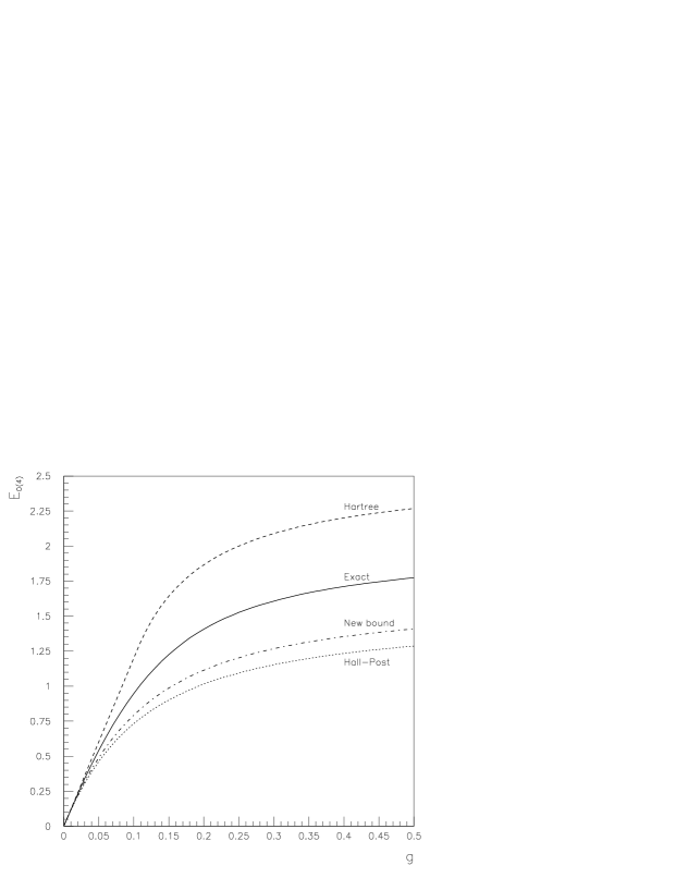
FIG. 3.: See caption Fig. 1. Case of repulsive pairing.

FIG. 4.: Ground-state energy $E_{0(A)}$ for $A=1000$ bosons with hamiltonian (92) in 50 harmonic oscillator levels. Dashed line: Hartree upper bound. Dotted line: Hall-Post lower bound ${\cal L}_{0}$. Dot-dashed line: improved lower bound ${\cal L}_{\tilde{\mu}}$, where $\tilde{\mu}=1$ or $\tilde{\mu}=2$ (see text).

FIG. 5.: Lower bounds for the energy of a system of $A$ bosons interacting with a power-law potential $\mbox{sgn}(\beta)r^{\beta}$. Solid line: relative improvement $R=({\cal L}_{1}-{\cal L}_{0})/\mid{\cal L}_{0}\mid$. The ratio $R=R_{1}R_{2}$ is a product of two factors (see Eq.(105)), which are also plotted. Dashed line: $R_{1}=1-S_{0(2)}^{\mbox{max}}/3$. Dotted line: $R_{2}=(\eta_{1(2)}-\eta_{0(2)})/\mid\eta_{0(2)}\mid$.

REFERENCES

• [1] J.L. Basdevant, A. Martin, and J.M. Richard, Nucl. Phys. B 343, 60 (1990); Nucl. Phys. B 343, 69 (1990)
• [2] J.M. Richard, and S. Fleck, Phys. Rev. Lett. 73, 1464 (1994)
• [3] J. Goy, J.M. Richard, and S. Fleck, Phys. Rev. A 52, 3511 (1995)
• [4] S. Moszkowski, S. Fleck, A. Krikeb, L. Theussl, J.M. Richard, and K. Varga, Phys. Rev. A 62, 032504 (2000)
• [5] D.K. Gridney, and J.S. Vaagen, Phys. Rev. C 61, 054304 (2000)
• [6] M.E. Fischer, and D. Ruelle, J. Math. Phys. 7, 260 (1966)
• [7] F.J. Dyson, and A. Lenard, J. Math. Phys. 8, 423 (1967); J. Math. Phys. 8, 621 (1967)
• [8] J.M. Lévy-Leblond, J. Math. Phys. 10, 806 (1969)
• [9] R.L. Hall, and H.R. Post, Proc. Phys. Soc. London 90, 381 (1967)
• [10] R.L. Hall, Proc. Phys. Soc. London 91, 16 (1967)
• [11] J.L. Basdevant, A. Martin, J.M. Richard, and T.T. Wu, Nucl. Phys. B 393, 111 (1993)
• [12] A. Benslama, A. Metatla, A. Backkhaznadji, S.R. Zouzou, A. Krikeb, J.L. Basdevant, J.M. Richard, and T.T. Wu, Few-Body Systems 24, 24 (1998)
• [13] O. Juillet, S. Fleck, L. Theussl, J.M. Richard, and K. Varga, preprint xxx.lanl.gov/quant-ph/0008048 (2000)
• [14] D. Van Neck and M. Waroquier, Phys. Rev. C 58, 3359 (1998)
• [15] D. Van Neck, A.E.L. Dieperink, and M. Waroquier, Phys. Rev. C 53, 2231 (1996)
• [16] D.S. Koltun, Phys. Rev. Lett. 28, 182 (1972)
• [17] J.J. Kelly, Adv. Nucl. Phys. 23, 75 (1996)
• [18] D. Van Neck, M. Waroquier, A.E.L. Dieperink, S.C. Pieper and V.R. Pandharipande, Phys. Rev. C 57, 2308 (1998)
• [19] A.E.L. Dieperink and T. de Forest Jr., Phys. Rev. C 10, 543 (1974)
• [20] Feng Pan, J.P. Draayer, and W.E Ormand, Phys. Lett. B 422, 1 (1998)
• [21] J. Dukelsky, and P. Schuck, preprint xxx.lanl.gov/cond-mat/0009057
• [22] R.W. Richardson, J. Math. Phys. 9, 1327 (1968)
• [23] R.L. Hall, J. Phys. G 26, 981 (2000)