Correlations in Many-Body Systems with Two-time Green’s Functions

Abstract

The Kadanoff-Baym (KB) equations are solved numerically for infinite nuclear matter. In particular we calculate correlation energies and correlation times. Approximating the Green’s functions in the KB collision kernel by the free Green’s functions the Levinson equation is obtained. This approximation is valid for weak interactions and/or low densities. It relates to the extended quasi-classical approximation for the spectral function. Comparing the Levinson, Born and KB calculations allows for an estimate of higher order spectral corrections to the correlations. A decrease in binding energy is reported due to spectral correlations and off-shell parts in the reduced density matrix.

]

I Introduction

The quantum Kadanoff-Baym equations (KB) [1] describe the time-evolution of the two-time (one-particle) Green’s functions $G({\bf p},t,t^{\prime})$. Imposing various approximations they have played an important role in the past developing corrections to the classical Boltzmann equation such as memory-effect and damping. With some restrictions it is now however feasible to solve these equations numerically without approximations.

We like to emphasize the following differences between the Boltzmann and KB-equations. In the quasi - classical Markovian Boltzmann-equation correlations are explicitly neglected. The spectral functions are given by the quasi-particle approximation. The kinetic energy is conserved in each binary collision, while the correlation energy is neglected. The equilibrium density-distribution (in momentum space) is a Fermi-distribution. Oppositely, in the KB-equations correlations are carried by the two-time Green’s functions. The total energy including the interaction potential energy is conserved. The reduced density distribution is given by a frequency integral of a spectral-function of non-zero width and a distribution function. At equilibrium this distribution-function is again given by a Fermi-distribution.

The various approximations of the KB-equations differ essentially by the reduction schemes of the two - time Green’s function to the reduced density matrix or even to the quasiparticle distribution. That this reduction is nontrivial can be traced to the fact that the Fermi and quasi-particle distributions decrease exponentially with energy while the reduced density matrix possesses power tails. In this paper we address some common schemes from the numerical point of view.

Numerical results of the quantum KB-equations already have been compared in the past with the classical Markovian dynamics as well as with other frequently used approximations [2, 3]. The study was made in particular with reference to collisions between heavy ions usually studied with the Boltzmann-equation or the BUU,VUU etc versions thereof. The general conclusion of the study was that quantum-effects reduce relaxation-rates by a factor as small as one half. This fact can be interpreted as being due to the pole renormalization or wave function renormalization [4].

Since the first numerical applications of the KB-equations by Danielewicz [2] several contributions to this evolving new field have been published with applications to nuclear matter [5, 3, 6, 7], to one- and two-band semiconductors [8, 9],to phonon-production in e-e collisions in plasmas [10] as well as to electron plasmas in general [11, 12]. Details of the computational methods is published in Computer Physics Communications[13].

The KB-equations are designed to study time-dependent non-equilibrium phenomena but they can also be used to study the system in its final equilibrium state. An example is found in [5] where an initially un-correlated zero-temperature Fermi-distribution time-develops into a correlated system whilst the collisions are calculated with the time-evolving correlated Green’s functions. The build-up of correlations is manifested as an asymptotic decrease in potential (correlation) energy (initially zero), with a corresponding increase in kinetic energy, while the total energy is constant. The resulting Green’s functions contain a wealth of information such as correlation energy and particle distribution. Spectral functions are also easily derived. Although the collision term basically implies a second order calculation with respect to the potential the propagators are by the process of time-iteration dressed with second order insertions (with their proper energy-dependence) up to all orders.

In this paper we further address and explore these features of the KB-equations. In particular we focus on correlation times and energies. We also extend previous comparisons[14] with the Levinson equation. This equation can be obtained from the KB-equations by approximating the propagators in the collision integral by free Green’s functions. The comparison between the two approaches allow us then not only to explore the validity of the Levinson equation but also to asses the importance of the higher order diagrams associated with the dressing of the propagators.

Although the interaction can in principle be a T-matrix, including ladder summations, the presented calculations are done with an effective time - local interaction. Section 2 contains a short summary of the KB-formalism used in this paper. Section 3 deals with the Levinson equation and some relations involving correlation energies and the Born approximation are shown. An apparent dilemma concerning the Born approximation result in Section 3 is resolved in Section 4 using the extended quasiparticle picture. Numerical results are shown in Section 5 and Section 6 summarizes our findings.

II The KB-equations

We show some of the equations regarding the KB-formalism needed for our presentation. For further details see for example refs[1, 2, 15].

In a homogeneous medium neglecting the mean field the KB-equations reduce (with $\hbar=1$) to:

$$(i{\partial\over{\partial t}}-{p^{2}\over{2m}})G^{{}^{>}_{<}}({\bf p},t,t^{\prime})=$$ (1)

$$\int_{t_{0}}^{t}dt^{\prime\prime}(\Sigma^{>}({\bf p},t,t^{\prime\prime})-\Sigma^{<}({\bf p},t,t^{\prime\prime}))G^{{}^{>}_{<}}({\bf p},t^{\prime\prime},t^{\prime})-$$ (2)

$$\int_{t_{0}}^{t^{\prime}}dt^{\prime\prime}\Sigma^{{}^{>}_{<}}({\bf p},t,t^{\prime\prime})(G^{>}({\bf p},t^{\prime\prime},t^{\prime})-G^{<}({\bf p},t^{\prime\prime},t^{\prime}))$$ (3)

(4)

$$(-i{\partial\over{\partial t^{\prime}}}-{p^{2}\over{2m}})G^{{}^{>}_{<}}({\bf p},t,t^{\prime})=$$ (5)

$$\int_{t_{0}}^{t}dt^{\prime\prime}(G^{>}({\bf p},t,t^{\prime\prime})-G^{<}({\bf p},t,t^{\prime\prime}))\Sigma^{{}^{>}_{<}}({\bf p},t^{\prime\prime},t^{\prime})-$$ (6)

$$\int_{t_{0}}^{t^{\prime}}dt^{\prime\prime}G^{{}^{>}_{<}}({\bf p},t,t^{\prime\prime})(\Sigma^{>}({\bf p},t^{\prime\prime},t^{\prime})-\Sigma^{<}({\bf p},t^{\prime\prime},t^{\prime})).$$ (7)

(8)

The notations are the conventional ones. $G^{>}$ and $G^{<}$ are essentially the occupation-numbers for holes and particles respectively. The particle distribution function $\rho({\bf p},t)$ is given by

$$\rho({\bf p},t)=-iG^{<}({\bf p},t,t).$$ (9)

The Green’s functions $G^{>}$ and $G^{<}$ are related on the diagonal in the $t,t^{\prime}$ plane by

$$G^{>}({\bf p},t,t)=-i+G^{<}({\bf p},t,t).$$ (10)

Between these two Green’s functions there exists a useful relation

$$G^{{}^{>}_{<}}({\bf p},t,t^{\prime})=[G^{{}^{>}_{<}}({\bf p},t^{\prime},t)]^{*}.$$ (11)

The scattering rates $\Sigma$ are given by

$$\Sigma^{{}^{>}_{<}}({\bf p},t,t^{\prime})=-i\int{d^{3}{\bf p_{1}}\over{(2\pi)^{3}}}G^{{}^{<}_{>}}({\bf p_{1}},t^{\prime},t)$$ (12)

$$\times\left<{1\over{2}}({\bf p-p_{1}})\mid T^{{}^{>}_{<}}({\bf p+p_{1}},t,t^{\prime})\mid{1\over{2}}({\bf p-p_{1}})\right>.$$ (13)

Here $T^{{}^{>}_{<}}$ is defined by

$$\left<{\bf p}\mid T^{{}^{>}_{<}}({\bf P},t,t^{\prime})\mid{\bf p}\right>=$$ (14)

$$\int dt^{\prime\prime}dt^{\prime\prime\prime}d{\bf p^{\prime\prime}}d{\bf p^{\prime\prime\prime}}\left<{\bf p}\mid T^{+}({\bf P},t,t^{\prime\prime})\mid{1\over{2}}({\bf p^{\prime\prime}-p^{\prime\prime\prime}})\right>$$ (15)

$$\times G^{{}^{>}_{<}}({\bf p^{\prime\prime}},t^{\prime\prime},t^{\prime\prime\prime})G^{{}^{>}_{<}}({\bf p^{\prime\prime\prime}},t^{\prime\prime},t^{\prime\prime\prime})$$ (16)

$$\times\left<{1\over{2}}({\bf p^{\prime\prime}-p^{\prime\prime\prime}})\mid T^{-}({\bf P},t,^{\prime\prime\prime}t^{\prime})\mid{\bf p}\right>.$$ (17)

The effective interaction $T^{\pm}$ is usually defined in a binary collision (ladder) approximation by an integral equation formally written as

$$T^{\pm}_{12}=V+VG^{\pm}_{1}G^{\pm}_{2}T^{\pm}_{12}$$ (18)

where $V$ is the ’free’ interaction potential.

In the following $T^{\pm}$ will be approximated by a local time-independent effective interaction

$$V({\bf p})=\pi^{3/2}\eta^{3}V_{0}e^{-\frac{1}{4}\eta^{2}p^{2}}$$ (19)

with $\eta=0.57fm$ and $V_{0}=-453MeV$. Considering the full dynamical T-matrix approximation one obtains more involved time integrals which gives rise to nonlocal effects [4, 16, 17].

The exchange term is not included. The eq. (13) for the scattering rates then simplifies to

$$\Sigma^{{}^{>}_{<}}({\bf p},t,t^{\prime})=-i\int{{d^{3}{\bf p_{1}}d^{3}{\bf q}}\over{(2\pi)^{6}}}V^{2}({\bf q})$$ (20)

$$\times G^{{}^{<}_{>}}({\bf p_{1}},t^{\prime},t)G^{{}^{>}_{<}}({\bf q+p_{1}},t,t^{\prime})G^{{}^{>}_{<}}({\bf p-q},t,t^{\prime}).$$ (21)

The momentum integrations are conveniently evaluated using the convolution theorem for Fourier transforms. The diagrammatic representation can be seen in figure 1. We will compare in the paper the selfconsistent with the non-selfconsistent approximation which are given in figure 1 by thick and thin lines respectively.

The total energy of the system reads [1]

$$E_{\rm tot}(t)={1\over{2}}K_{\rho}(t)+{1\over{4}}\int{{d^{3}{\bf p}}\over{(2\pi)^{3}}}({\partial\over{\partial t_{1}}}-{\partial\over{\partial t_{2}}})G^{{}^{<}}({\bf p},t_{1},t_{2}))$$ (22)

which is used throughout the paper for calculating the total energy. The kinetic energy $K_{\rho}$ for the correlated medium is

$$K_{\rho}(t)=\int{{d^{3}{\bf p}}\over{(2\pi)^{3}}}{p^{2}\over{2m}}\rho({\bf p},t)$$ (23)

and the correlation energy is defined by

$$E_{\rm corr}(t)=E_{\rm tot}(t)-K_{\rho}(t).$$ (24)

Note that the mean or Hartree-Fock field is not included in our work and the total energy therefore contains only the correlated energy. We also define the uncorrelated kinetic energy by

$$K_{f}(t)=\int{{d^{3}{\bf p}}\over{(2\pi)^{3}}}{p^{2}\over{2m}}f({\bf p},t).$$ (25)

The relation between the reduced density matrix $\rho$ and the quasi-particle distribution $f$ will be discussed below. (See Section 4) Several numerical applications of this formalism are published. For some references see the Introduction. A detailed description of numerical details are published in ref.[13].

FIG. 1.: The integral form of Kadanoff-Baym equation (above) and the two discussed approximations for the selfenergy (below). The first line describes the selfconsistent Born approximation (thick lines) and the second line the non-selfconsistent Born approximation (thin lines). The latter one leads to the Levinson equation (35).

In this paper we concentrate on correlation energies and correlation times. All (with one exception) calculations are performed with an initially uncorrelated nuclear matter system and a momentum-distribution $f({\bf p},t=0)$ specified by a density $\rho$ and temperature T. The system is then time-evolved beyond equilibrium. The selfenergies are conserving[1, 18] so that the total energy is conserved. Therefore we have during the time evolution

$$K_{f}^{i}=E_{\rm tot}(t)=E^{\rm eq}_{\rm tot}$$ (26)

where $K_{f}^{i}$ is the kinetic (and total) energy of the initial unperturbed and uncorrelated system and $E^{\rm eq}_{\rm tot}$ is the total energy after equilibration ($t\rightarrow\infty$) including correlations.

III The Levinson equation

As we will show below the Levinson equation can be considered as one of several proposed approximations of the KB-equations. It is of particular interest to us here because it allows for some analytic results [33, 14] that help to understand the numerical findings and also help to illustrate some important features built into the KB-equations. Let us first discuss different reduction schemes of the KB equation including the Levinson equation.

To evolve the two-time KB-equations along $t=t^{\prime}$ one needs the Green’s functions for off-diagonal times $t\neq t^{\prime}$. Different methods have been proposed approximating the off-diagonal elements in terms of the diagonal ones and using eq.(9) a one-time theory can then be derived.

The first method we want to discuss is the Generalized Kadanoff Baym (GKB)-ansatz introduced by Lipavsky et al. [19] given by

$$G^{<}({\bf p},t,t^{\prime})=G^{<}({\bf p},t,t)S({\bf p},t,t^{\prime})$$ (27)

for $t^{\prime}>t$ and

$$G^{>}({\bf p},t,t^{\prime})=G^{>}({\bf p},t^{\prime},t^{\prime})S({\bf p},t,t^{\prime})$$ (28)

for $t>t^{\prime}$. $S$ is the spectral function defined by

$$S({\bf p},t,t^{\prime})=i(G^{>}({\bf p},t,t^{\prime})-G^{<}({\bf p},t,t^{\prime})).$$ (29)

The GKB ansatz was discussed in ref [5] and numerical results were also shown of various approximation schemes. The very simplest ansatz for the spectral function is the quasiparticle approximation to get

$$G^{<}({\bf p},t,t^{\prime}) = G^{<}({\bf p},t,t)e^{i\omega(t-t^{\prime})}$$ (30)

$$G^{>}({\bf p},t,t^{\prime}) = (-i+G^{<}({\bf p},t^{\prime},t^{\prime}))e^{-i\omega(t-t^{\prime})}.$$ (31)

The KB-equations then reduce to Levinson’s equation [3, 20, 21, 22] for homogeneous systems

$$\frac{\partial}{\partial t}{\rho}({\bf p},t)=$$ (32)

$$2\int\frac{d^{3}{\bf p}_{1}d^{3}{\bf p}^{\prime}d^{3}{\bf p}_{1}^{\prime}}{(2\pi)^{6}}V(\mid{\bf p}-{\bf p}^{\prime}\mid)^{2}\delta({\bf p}+{\bf p}_{1}-{\bf p}^{\prime}-{\bf p}_{1}^{\prime})$$ (33)

$$\times\int_{t_{0}}^{t}d\tau{\rm cos}\Delta\omega(t-\tau)({\rho}({\bf p}^{\prime},\tau){\rho}({\bf p}_{1}^{\prime},\tau){\bar{\rho}}({\bf p},\tau){\bar{\rho}}({\bf p}_{1},\tau)$$ (34)

$$-{\rho}({\bf p},\tau){\rho}({\bf p}_{1},\tau){\bar{\rho}}({\bf p}^{\prime},\tau){\bar{\rho}}({\bf p}_{1}^{\prime},\tau))$$ (35)

with $\bar{\rho}=1-{\rho}$ and $\Delta\omega=(\omega+\omega_{1}-\omega^{\prime}-\omega_{1}^{\prime})$ . The mean field is neglected in the following and the quasiparticle energy is approximated by an effective mass $\omega=p^{2}/2m$. If for large times the distribution function becomes stationary the integration over the cos-function reduces to $\delta(\Delta\omega)$ and the equilibrium distribution $\rho$ will be a Fermi-distribution.[14]

By the approximation (31) the correlated (damped) Green’s functions in the KB-equations are replaced by the free Green’s functions which in other words means that the second order energy diagram is calculated without insertions in the particle (hole) lines.(See Fig. 1). In the time-evolution of the KB-equations the lines are on the other hand dressed repeatedly with $V^{2}$ insertions. This results in a damping or dephasing while there is no damping in the Levinson equation but there does remain a memory-effect; the integration over $\tau$ in eq (35).

It is instructive to notice that the Boltzmann collision integral is obtained from equation (32) if:
(i) One neglects the time retardation in the distribution functions, i.e. the memory effects and
(ii) The finite initial time $t_{0}$ is set equal to $-\infty$ corresponding to what is usually referred to as the limit of complete collisions.

For the Markovian Boltzmann equation the kinetic energy is conserved, while the potential energy is zero. The Levinson equation conserves the total energy. [23] The correlation energy is now given by

$$E_{\rm corr}(t)=$$ (36)

$$-\frac{1}{4}\int\frac{d^{3}{\bf p}d^{3}{\bf p}_{1}d^{3}{\bf p}^{\prime}d^{3}{\bf p}_{1}^{\prime}}{(2\pi)^{9}}V(\mid{\bf p}-{\bf p}^{\prime}\mid)^{2}\delta({\bf p}+{\bf p}_{1}-{\bf p}^{\prime}-{\bf p}_{1}^{\prime})$$ (37)

(38)

$$\times\int_{t_{0}}^{t}d\tau{\rm sin}\Delta\omega(t-\tau)({\rho}({\bf p}^{\prime},\tau){\rho}({\bf p}_{1}^{\prime},\tau){\bar{\rho}}({\bf p},\tau){\bar{\rho}}({\bf p}_{1},\tau)$$ (39)

$$-{\rho}({\bf p},\tau){\rho}({\bf p}_{1},\tau){\bar{\rho}}({\bf p}^{\prime},\tau){\bar{\rho}}({\bf p}_{1}^{\prime},\tau)).$$ (40)

For large times eq. (40) reduces to [14]

$$E_{\rm corr}^{\rm eq}=$$ (41)

$$-\frac{1}{2}\int\frac{d^{3}{\bf p}d^{3}{\bf p}_{1}d^{3}{\bf p}^{\prime}d^{3}{\bf p}_{1}^{\prime}}{(2\pi)^{9}}V(\mid{\bf p}_{1}-{\bf p}_{1}^{\prime}\mid)^{2}\delta({\bf p}+{\bf p}_{1}-{\bf p}^{\prime}-{\bf p}_{1}^{\prime})$$ (42)

$${\rho}_{eq}({\bf p}_{1}^{\prime}){\rho}_{eq}({\bf p}_{2}^{\prime}){\bar{\rho}_{eq}}({\bf p}_{1}){\bar{\rho}_{eq}}({\bf p}_{2}){{\cal P}\over{\Delta\omega}}$$ (43)

where $\cal P$ denotes the principal value and where $\rho_{eq}$ indicates the equilibrium large time correlated densities. This energy resembles the second order Born estimate of the potential energy but with two important differences.

The first of these is that the densities $\rho_{eq}$ are correlated densities, in the long time equilibrated limit. A Born estimate would however be done with an uncorrelated distribution $f$. For weak interactions and/or low density for which the Levinson equation and the Born approximation are certainly valid, the difference between initial uncorrelated and final correlated densities is negligible. Around nuclear matter values this difference is however important and we shall address this question below showing numerical results for Levinson densities, KB densities as well as initially uncorrelated densities.

The second difference between eq. (41) and the second order Born estimate is that upon closer inspection a factor of one-half appears missing. This will now be clarified. With the correlation energy given by eq. (41) the total energy after equilibration is using eq. (24)

$$K_{f}^{i}=E^{\rm eq}_{\rm tot}=K_{\rho}^{\rm eq}+E_{\rm corr}^{\rm eq}$$ (44)

The second order Born approximation for the total energy is on the other hand known from perturbation theory

$$E_{tot}^{eq}=E_{Born}=K_{f}^{eq}+{1\over{2}}E_{\rm corr}^{\rm eq}.$$ (45)

(As noted above the Hartree-Fock energy is not included so that accordingly the first order contribution to the energy is not included here.) One should note that in the process of equilibration the system is excited and the correlation energy does in both expressions (44) and (45) refer to the excited but not to the initial ground state of nuclear matter. Also note that in the process of excitation the uncorrelated kinetic energy $K_{f}^{i}$ has increased to $K_{f}^{eq}$.

In order to resolve the apparent disagreement between eqs. (44) and (45) we first note that eq. (44) results from a time-evolution of the Levinson equation starting from an uncorrelated system with a kinetic energy $K_{f}^{i}$. We shall show below that the correlated and uncorrelated kinetic energies at the end of the time-evolution are related by

$$K_{\rho}^{\rm eq}=K_{f}^{\rm eq}-{1\over{2}}E_{\rm corr}^{\rm eq}$$ (46)

Upon insertion in eq. (44) the apparent disagreement is then resolved.

To prove eq. (46) we have to discuss the difference between the reduced density matrix $\rho$ and the quasiparticle distribution $f$. This is performed in the extended quasiparticle picture.

IV Extended quasiparticle picture

In the previous section we derived the Levinson equation from the time diagonal parts of the Kadanoff and Baym equations. We adopted the GKB ansatz for the closure of the off-diagonal parts of the Green’s functions. But there is another path that we now want to explore.

Our alternative is to use the extended quasiparticle approximation (EQP) for the spectral function in the final equilibrated system. The EQP is consistent with the Levinson equation as both are a low density and/or weak interaction approximation but they differ in their physical content and different renormalizations [24]. In an expansion with $Im\Sigma^{+}<<Re\Sigma^{+}$ and $\partial Re\Sigma^{+}/\partial\omega<<1$ one finds[15, 25, 26] for the spectral function

$$S_{EQP}({\bf p},\omega)=2\pi\delta(\omega-\omega_{0})Z({\bf p})-{\cal P}{2Im\Sigma^{+}({\bf p},\omega)\over{(\omega-\omega_{0})^{2}}}$$ (47)

where

$$Z({\bf p})=1+({\partial Re\Sigma^{+}({\bf p},\omega)\over{\partial\omega}})_{\omega=\omega_{0}}$$ (48)

is the wave function renormalization and where ${\cal P}$ indicates that the principal value is to be taken when integrating over $S$. The energy $\omega_{0}$ is defined by

$$\omega_{0}=p^{2}/2m+Re\Sigma^{+}({\bf p},\omega_{0})$$ (49)

and $\Sigma^{+}$ is the retarded selfenergy.(See also Sect. 5.2). The EQP approximation satisfies the first two $\omega$ weighted sum rules [4].

$$\int{d\omega\over 2\pi}S_{EQP}({\bf p},\omega) = 1$$ (50)

$$\int{d\omega\over 2\pi}\omega S_{EQP}({\bf p},\omega) = {{\bf p}^{2}\over 2m}+\Sigma_{HF}({\bf p})$$ (51)

and has been well tested numerically for nuclear matter[25].

In equilibrium the expansion (47) is consistent with the following ansatz

$$G^{<}({\bf p},\omega)=if({\bf p})2\pi Z({\bf p})\delta(\omega-\omega_{0})+\Sigma^{<}({\bf p},\omega){{\cal P}\over{(\omega-\omega_{0})^{2}}}.$$ (52)

It allows for an approximate construction of the Green’s function and the Wigner or reduced density matrix in terms of the quasiparticle distribution. The relation between these two distribution functions, the quasiparticle distribution and the reduced density matrix, was first introduced by Craig [27] within the limit of small scattering rates. An inverse functional $f[\rho]$ was constructed in ref. [28]. For equilibrium nonideal plasmas the correlated density has been employed in refs. [15, 29] and under the name of the generalized Beth-Uhlenbeck approach it has been used in ref. [30] for nuclear matter studies. The authors in refs. [25, 26] have used this approximation under the name of Extended Quasiparticle Approximation for the study of the mean removal energy, reduced density and high-momenta tails of the reduced density matrix.

The non-equilibrium (time-dependent) extension of this formalism has been recovered within the quasiparticle approach to the kinetic equation for weakly interacting particles and referred to as a modified Kadanoff and Baym ansatz [31, 32].

Integrating eq. (52) (in the time-dependent extension) over $\omega$ gives a relation between the reduced density matrix and the quasiparticle distribution

$$\rho({\bf p},t)=f({\bf p},t)Z({\bf p},t)-i\int{d\omega\over{2\pi}}\Sigma^{<}({\bf p},\omega,t){{\cal P}\over{(\omega-\omega_{0})^{2}}}.$$ (53)

The imaginary part of the retarded function $\Sigma^{+}$ is obtained from

$$Im\Sigma^{+}({\bf p},\omega,t)=-{i\over{2}}(\Sigma^{>}({\bf p},\omega,t)-(\Sigma^{<}({\bf p},\omega,t))$$ (54)

and the real part is obtained from the dispersion relation. Then

$$Z({\bf p},t)=1-i\int{d\omega\over{2\pi}}{{\cal P}\over{(\omega-\omega_{0})^{2}}}(\Sigma^{<}({\bf p},t)-\Sigma^{>}({\bf p},t))$$ (55)

so that eq. (53) can be rewritten as

$$\rho({\bf p},t)=f({\bf p},t)-i\int{d\omega\over{2\pi}}{{\cal P}\over{(\omega-\omega_{0})^{2}}}$$ (56)

$$\times(\Sigma^{<}({\bf p},\omega,t)(1-f({\bf p},t))+\Sigma^{>}({\bf p},\omega,t)f({\bf p},t))$$ (57)

providing also the relation between the uncorrelated and correlated energies. Multiplying with the kinetic energy ${p^{2}\over{2m}}$ and integrating over ${\bf p}$ one finds the relation (46) that we wanted to prove.

We like to point out that the first term in eq (57) is just the uncorrelated distribution while the second corrects for the off-shell scatterings. It was shown in ref [25] that this equation gives practically exact agreement with a Brueckner calculation. One should also note that the Levinson equation for the reduced density-matrix was derived with the ansatz (31) i.e. with a quasi-particle spectral function. The correlations induced in the time-evolution then result in a spectral function consistent with the EQP-approximation. If one instead uses the EQP spectral function in the ansatz the result is a nonlocal Boltzmann - like kinetic equation for the quasiparticle distribution [16, 17]. For the frequency independent real valued interaction used here the nonlocal effects vanish and we are left with the Boltzmann equation for the quasiparticle distribution $f$ from which one then can find the reduced density matrix by (57). Alternatively one can consider the Levinson equation for the reduced density matrix directly. This is the approach taken in this paper. For more detailed discussions, derivations and physical content of these relations we refer the reader to refs [4, 24].

Let us remind that the two outlined schemes, the Levinson equation as well as EQP, are strictly valid only at low density and/or for weak interactions. All the same, the EQP has been found to be an excellent approximation for nuclear matter[25].

V Numerical results

In the above we have displayed the KB- as well as the Levinson-equations; the latter is obtained from KB using free (quasi-particle) Green’s functions in the collision kernel.

In this section we show some results of our calculations. The equations (KB and Levinson) were time-evolved starting at time $t=0$ with an uncorrelated Fermi gas of specified density and temperature. In addition to KB and Levinson correlation energies we have also calculated the second order Born energy given by eq. (41). In one case we also consider the collision between two Fermi-spheres (slabs in coordinate-space).

A comparison with the approximate Levinson and Born results requires a high precision of the calculations to be meaningful. To minimize the relative errors all calculations are made with essentially the same KB computer-program. To perform the Levinson calculations all that has to be changed relative to the KB is to replace the selfconsistently calculated Green’s functions used in the KB-code in the collision-kernel with the free Green’s functions shown in eq (31). In the second order Born-approximation calculations the Green’s functions on the time-diagonal were replaced by constant (time-independent) distribution functions $\rho({\bf p})$ as specified in the respective calculations below.

It may be noteworthy to point out that the Pauli-blocking which in most perturbative calculations such as Brueckner is treated approximately (e.g. with an angle averaging) here is treated ”exactly”.

The meshes that we use are an improvement relative to previous work as more computer-power is now available. The momentum-mesh in the Cartesian coordinate system that we use was 57 points along each axis with $\Delta p_{x}=\Delta p_{y}=\Delta p_{z}=0.2fm^{-1}$. The number of time-steps was typically $80$ with $\Delta t=0.25fm/c$ . The interaction shown in eq. (19) was used. The dependence of the strength $V_{0}$ of the interaction is now also investigated.

A Approach to Equilibrium; Correlation Times

If one time-evolves an initially uncorrelated Fermi-distribution with the classical Boltzmann-equation (modified for Fermion-statistics) this initial distribution would be stationary. The Fermi-distribution is in fact a solution of this equation with the collision-term equal to zero. There are no two-body correlations. This is not so for the Kadanoff-Baym equation. As the system in this case evolves from the initial uncorrelated state the correlation energy decreases with time. The system correlates. At the same time the kinetic energy increases by the same amount, because our choice of self-energies is conserving i.e. the total energy is conserved. As a consequence of the self-consistent time-iterations higher and higher orders of insertion diagrams are included in the Green’s function propagators until full selfconsistency and equilibration is achieved. In the KB-case the system converges to an equilibrated distribution but this is not always so for the Levinson-case. We shall return to this below.

In a previous publication[14] we have already considered the correlation time $t_{c}$, i.e. the time it takes the system to correlate time-evolving from the initially uncorrelated Fermi-distribution. It was in particular found that in the Levinson-approximation a simple result could be derived at low temperature namely

$$t_{c}={1\over{E_{F}}}$$ (58)

with $E_{F}$ the Fermi-energy. The temperature-dependence was found to be relatively small. This result was also used in a subsequent paper on interferometry methods[34].

Fig. 2 shows the correlation energies normalized to the equilibrium energy as a function of time for five different densities as indicated in the figure-caption. The initial distribution is in each case a zero temperature Fermi-distribution.

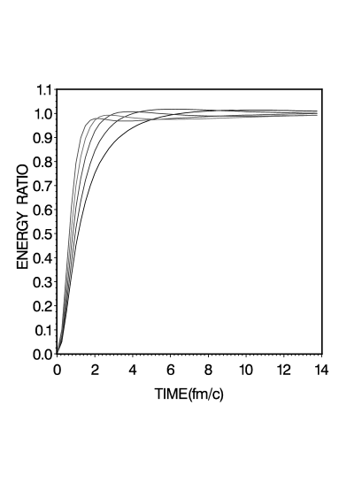
FIG. 2.: Correlation energy from KB-calculations as a function of time normalized to final equilibration energies. From left to right the five curves correspond to the normal density of nuclear matter ($\rho_{0}=0.18fm^{-3}$) multiplied by $2,1,0.5,0.25$ and $0.125$. See also Table I

In accordance with ref. [14] we define the correlation times $t_{c}$ as the time of maximum correlation-energy. We now find that the times $t_{c}$ scale roughly as

$$t_{c}={1\over{2E_{F}}}$$ (59)

as shown in Table I. The previous analytic result (58) based on the Levinson equation gave correlation times twice as large. A precise definition of these times is however not possible as is also seen in figure 2.

Fig. 3 shows the correlation energies normalized to the equilibrated energy at five different interaction-strengths indicated in the figure-caption. The initial distribution is in each case a zero-temperature Fermi-distribution. The previous analytic finding [14]was that the correlation times are roughly independent of the interaction strengths. This is nicely confirmed by the numerical results of Fig. 3 for times smaller than $2$ fm/c. There is however a large overshoot as the strength is decreased. This still remains to be understood. With the particular definition of the correlation-times that we have adopted we still see a dependence on the interaction-strengths because of this overshoot as displayed in Table III.

FIG. 3.: Similar to Fig. 2 but for normal nuclear matter density and different interaction strengths. The normal strength $V_{0}=453$ is multiplied by $2.0,1.0,0.5.0.25$ and $0.125$ respectively. The figure shows t there is an increasing ”overshoot” of the correlation energy as the strength is decreased. See also Table III

In a previous paper it was also shown that the temperature dependence of $t_{c}$ should be quite small. [14] This conclusion was based on the Levinson equation. The result using the KB-equations shown in Fig. 4 confirms this. One may only note that the approach to equilibration is markedly different at higher temperatures as compared to zero temperature. Our general conclusion regarding the independence of temperature is also exemplified by the second curve from the left in Fig. 4. This shows the correlation energy in a ”collision” between two Fermi-spheres separated by a momentum of $2.2fm^{-1}$ (100 MeV/A collision energy) and with a total density of $0.18fm^{-3}$ (normal density).

In the calculations with the KB-equations our choice of selfenergies are conserving, i.e. total energy is conserved. [18] The Levinson-equations also conserve total energy. From our calculations we find after $80$ time-steps a decrease in total energy of $3.8\%$ at normal nuclear matter density and similarly an increase of $1.3\%$ in the KB-case. This numerical accuracy is quite satisfactory.

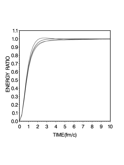
FIG. 4.: Correlation energy as a function of time normalized to final equilibration energies. The interaction strength and density are both normal. From left to right the first,third and fourth curves are for initial temperatures $0,20$ and $40$ MeV respectively. The second curve is for a ”collision” event (see text). Notice the near overlap of the curves.

Another important result shown by Figs 2-4 is that the correlation energy (and the kinetic energy) converges to an equilibrium value in the KB-case. While the KB-results show excellent convergence this is not true in the Levinson case as shown by Fig. 5 which should be compared with Fig. 3. One finds a convergence only for the two weakest interactions which also agree quite well with the corresponding curves in Fig. 3 while only moderate convergence with the factor $0.5$. For the strongest interaction there is even sign of an instability in agreement with the findings of Haug [35] and others [36],[37] who found a continuous increase of energy with time. The origin of this problem with the Levinson equation was discussed in terms of the artificial collisional broadening [38].

We note that in the Levinson case the Green’s functions are free, uncorrelated, in the collision-term while the ensuing Green’s functions are not free as e.g. evidenced by the non-zero potential energies. This is an inconsistency in the Levinson equation which, we believe, is related to the non-convergence. The problem with this equation is also reflected in the results in Table III showing reasonably good agreement between KB and Levinson correlation energies only for the three weakest interactions.

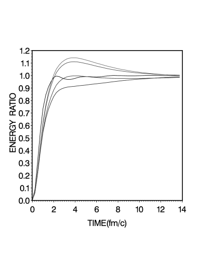
FIG. 5.: Time-dependence of normalized correlation energies in the Levinson-case for normal nuclear matter density. The oscillating curve is with the interaction strength twice the normal. The smooth curves from bottom and up are with strengths $1.,0.5,0.25$ and $0.125$ times the normal. Notice that the correlation energy converges only for the two weakest interactions. Compare with the KB-results in Fig. 3. The initial distribution is in each case a zero-temperature distribution of normal nuclear matter density.

The fact that the correlation time is finite and of the order of some $fm/c$ in nuclear matter is, we believe, of importance when studying heavy ion collisions. Correlations will change with density and temperature with typically this response time. In a previous paper we have already looked at the consequence of this fact on interferometry measurements.[34]

B Equilibrium Spectral Function; Occupation Numbers

Correlation energies are intimately related to the spectral functions in our case given by eq. (29). In the quasi-particle approximation valid for weak interactions and an uncorrelated medium they are simply delta-functions corresponding to vanishing widths represented by the first part of eq. (47).

In this section we consider the system in its final equilibrated state. The total energy is then related to the spectral function by

$$E_{\rm tot} = 2\int_{-\infty}^{+\infty}d\omega f(\omega)\int_{-\infty}^{+\infty}\frac{d^{3}{\bf p}}{(2\pi)^{3}}[{p^{2}\over 2m}+\omega]S({\bf p},\omega)$$ (60)

which is the same as eq. (22) with the equilibrium relations

$$G^{<}({\bf p},\omega) = iS({\bf p},\omega)f(\omega)$$ (61)

$$G^{>}({\bf p},\omega) = iS({\bf p},\omega)(1-f(\omega)).$$ (62)

A factor $4$ is included for the spin, isospin etc. degeneracy of the nuclear system.

The spectral functions $S({\bf p},\omega)$ can be calculated from eq. (29) by Fourier-transforming from the time-domain. It was found more practical however to use

$$\ S({\bf p},\omega)={2Im\Sigma^{+}({\bf p},\omega)\over{(\omega-{p^{2}\over{2m}}-Re\Sigma^{+}({\bf p},\omega))^{2}+(Im\Sigma^{+}({\bf p},\omega))^{2}}}.$$ (63)

Figure 7 shows some results at normal nuclear matter density. These are from KB-calculations. (As noted above in section 3 the spectral functions in the Levinson approximation are in agreement with the EQP-approximation (47) in lowest order densities.) The initial distribution is a zero-temperature Fermi-distribution and the $\omega$-dependent selfenergies are obtained by Fourier-transforming from the time-domain after equilibration. The correlation energy is in this case 35.95 MeV as shown in Table I. The figure shows that the widths are comparable with those from Brueckner and other many body calculations with ”realistic” interactions. If the calculation were for the ground-state the distribution would be much more peaked at this momentum. Because the calculations in our present work are made from an initially uncorrelated state that is then time-evolved along the real axis the final state corresponds to an excited state (with a temperature estimated to be about 25 MeV). For comparison we also show in fig. 6 spectral functions for the ground state obtained with imaginary time-stepping.[2, 5] The momenta at the Fermi-surface is not shown here as it would be too high and narrow in this case, but note the peaks at the adjacent momenta.

The occupation-numbers are in equilibrium also related to the spectral functions by

$$\rho({\bf p}) = {1\over{2\pi}}\int_{-\infty}^{+\infty}f(\omega)S({\bf p},\omega)d\omega$$ (64)

consistent with eqs. (9) and (62).

Figure 8 shows a comparison of the density-distributions obtained respectively from the KB- and Levinson calculations. Please note that the KB calculations lead to a pronounced discontinuity at the Fermi energy. A quasiparticle (Fermi-) distribution $f$ with a temperature of $27$ MeV is plotted for comparison. This is the roughly estimated temperature of the final equilibrated system. This would be the distribution in a Boltzmann calculation in which case there are no correlations, the spectral function is the quasi-classical and the $\rho$ and $f$ distributions are identical. The KB - as well as Levinson distributions possess power tails at high momenta and suppress states at lower momenta due to correlations[4].

Correlation energies are shown in Tables I and III. These are energies after $80$ time-steps ($20fm/c$). At this time the system is well equilibrated in the case of KB as already seen in the figures 2, 3 and 4. In other words the Green’s functions along the time-diagonal become constant for large times.

This is not so for the off-diagonal elements that carry the correlations. Fig 9 shows the absolute value of these elements normalized to the equilibrium value, as a function of past times. For the KB-calculations the well-known damping or dephasing is seen.

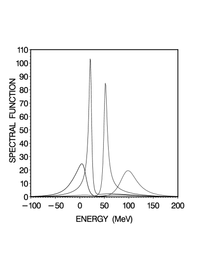
FIG. 6.: Similar to Fig 7 except that these spectral functions are for the ground-state and obtained with imaginary time-stepping. The momenta are from left to right $.0,1.0,1.6$ and $2.2fm^{-1}$.

The slight increase for the largest past times is a natural consequence of the correlation process. While the equilibrated occupation for $p=0$ is $0.62$. (See fig 8) the initial value was $1.0$ and this is still ”memorized” $20~{}fm/c$ later.

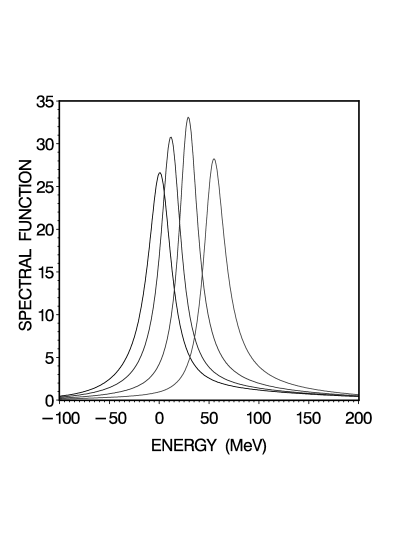
FIG. 7.: Spectral functions in nuclear matter at $\rho=0.18fm^{-3}$, $k_{f}=1.4fm^{-1}$. The momenta are from left to right $0.0,0.75,1.2$ and $1.65fm^{-1}$. Note that the last momentum is larger than $k_{f}$. The temperature is here estimated to be $25$  MeV.

Of particular interest is the increase in damping as the strength of the interaction is increased which is well illustrated by the figure. This is a very important effect that is contained in the KB-equations with the selfconsistently calculated Green’s functions. This has as a consequence that the memory-time decreases; the integration over past times which in principle should start at the time when interactions are switched on, ($t_{0}$ in eqs. (4 and 8)), can now be limited to about $5fm/c$ or less before the point of time of the evolution. Fig 9 in ref.[5] illustrates this point. Associated with an increase of the strength of the interaction is of course not only a decrease in memory-time but also an increase in the width of the spectral functions.

Only for the very weakest strength the damping is negligible. This is consistent with Table III that shows a good agreement between all methods for this case. If the situation were such that the evolution at the same time is sufficiently slow another limit is reached. The time-integration can now be done analytically the energy-spread decreases and collapses to a delta-function. The Boltzmann limit is reached.

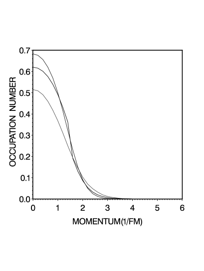
FIG. 8.: Density distributions from the KB- and Levinson- calculations at normal nuclear matter density. The KB-distribution is larger at small momenta and smaller at larger momenta. Notice that it shows the characteristic discontinuity at the Fermi-surface that is related to the strength-function. Compare with Fig. 1 in ref.(3) .

The Levinson curve is smooth (it is a Fermi-distribution) and starts at about $0.52$ at p=0. For comparison is also plotted an estimate of the Fermi-distribution $f$ with the same nuclear matter density and a temperature of $27$ MeV. It starts at about $0.68$.

The damping, so characteristic in the KB-case is absent in the Levinson case. The corresponding curves can increase or decrease in the latter case depending on the past distribution-function (on the time-diagonal). In the present calculations this function will always decrease for ${\bf p}=0$ and the plotted ratio in Fig. 9 is now consequently larger than 1.0.

C Equilibrium correlation energies

It was already shown above that the Levinson correlation energy for large times approaches a second order Born value. But it was also pointed out with reference to eq. (41) that the Born calculation then has to be made with the Levinson final reduced density but not with the initial quasiparticle distribution as would normally be done in a perturbative expansion. In the low-density and/or weak interaction limit, where the Born and Levinson approximations both become valid this difference should be irrelevant. This is verified by the results shown in columns 5,6 and 7 in table I showing Born energies calculated with occupation numbers from the KB, Levinson and initial distributions (labelled ”KB”,”Lev.” and ”Init.”) respectively. As expected the three energies agree exactly at the lowest density but the agreement becomes progressively worse as the density is increased. As predicted by eq. (41) the Born-column indicated ”Lev.” (column 6) agrees on the other hand nearly exactly with the Levinson result (column 4) at all densities, being a confirmation of computational accuracy.

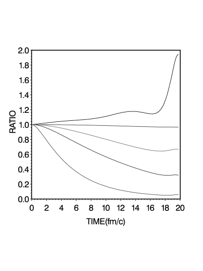
FIG. 9.: This figure shows the absolute value of $G^{<}({\bf p},T,t^{\prime})/G{<}({\bf p},T,T)$ for $T-t^{\prime}$ for four different strengths of the interaction. The four lower curves with the ratio less than 1.0 is from KB-calculations. From bottom to top the normal strength is multiplied by factors of $2.,1.,0.5$ and $0.125$. The uppermost curve is from Levinson calculation with normal interaction strength showing no damping but rather an increase with past times. This effect is explained in the text. The momentum is chosen to be ${\bf p}=0$ for all cases.

1 Comparison of Levinson with Born

As noted above the Born(Lev) correlation energies agree very well with the Levinson energies at all densities and temperatures but they differ from the Born(Init) energies as seen comparing columns 6 and 7 in table I. This is because the occupation-numbers differ in these two calculations. The Born(Init) calculations are made with the Fermi-distributions of the temperatures T indicated. These are also the initial distributions in the Levinson calculations, but the final distributions $\rho$ (with which also Born(Lev) is calculated) are different. There are two distinct effects contributing to the change from initial to final distribution. One is the heating associated with the correlations and the second comes from the difference between the reduced density matrix $\rho$ and the quasiparticle distribution $f$ that is contained in the off-shell part in EQP (57). We are going to discuss these two effects now.

The heating of the system in the Levinson case occurs since it correlates. The uncorrelated quasiparticle distribution $f$ is consequently of a higher temperature in the Born(Lev) case, column 6, than in the Born(Init) case, column 7.

In order to make a meaningful comparison between the two results we have to correct for this temperature-difference. Fortunately this is straightforward in the Levinson case. The numerical solution of the Levinson equation gives us the correlated distribution $\rho({\bf p},t)$ and from eq. (23) the kinetic energy $K_{\rho}(t)$ in the equilibrated medium (for large times). The relation (46) valid for the Levinson equation then gives us the kinetic energy $K_{f}^{\rm eq}$ which together with the density allows us to deduce the relevant parameters, temperature and chemical potential for the final equilibrium Fermi-distribution.

The Levinson correlation energy is then compared with the Born(Init) correlation energy calculated with that same final Fermi-distribution. The result of this comparison is shown in Table II at normal density. With the Born and Levinson calculations compared at the same temperature ($T_{f}$ in the table) i.e. with the same distribution $f(\omega)$ there is however a remaining difference, in Table II indicated by $Diff.$ We remind that when Born is calculated with the $\rho$-distribution (i.e. in Born(Lev)) rather than with the $f$-distribution we get no difference, i.e the Levinson energy. The remaining difference $Diff$ is then due to the second of the two separate effects referred to above. It is attributed to the difference between the reduced density $\rho$ and the corresponding quasiparticle distribution $f$. The former contains the spectral correction as in eqs. (53) and (64).

Such a spectral correction can be included in e.g. Brueckner type calculations by iteration but is rarely done. (See however a recent work [39]). Table II shows a decrease of $3.3MeV$ of the correlation energy at zero temperature. This implies a decrease in binding energy of $1.6MeV$. (We like to point out that in the EQP-approximation a change $\delta$ in correlation energy for a given distribution $f({\omega})$ changes the total energy by $\delta/2$. It changes the kinetic energy $K_{\rho}$ by $-\delta/2$.)

The dependence on the strength of the interaction is presented in Table III. The Born calculations are here for initial zero temperature Fermi distributions. For the three weakest interactions all three correlation energies agree reasonably well. But at full interaction strength we see differences of over 20 % increasing to 50 % at twice the strength.

2 Comparison of KB with Levinson

We now want to compare the KB- with the Levinson- equation. Although the KB collision term in our calculations is formally up to second order in the interaction the correlation energy at equilibrium is actually of a much higher (infinite) order. This is because the correlated Green’s functions are formed by iterative time-stepping functionals of the interaction.

The effect of these higher order terms can be assessed from comparing the KB and Levinson correlation-energies. The difference between the two stems from the difference between the Green’s functions in the collision kernel for the two separate cases. In the KB case they are selfconsistent (correlated) while in the latter they are free Green’s functions. In diagrammatic language the presence of the correlated Green’s functions in the collision kernel means that hole- and particle-lines are dressed with the two-point (second order) insertions to all orders and all time orderings, see Fig. 1. This implies that for a similar calculation in the $\omega$-representation the proper dependence on $\omega$ of the selfenergy $\Sigma^{+}({\bf p},\omega)$ has to be included in the calculation. The same problem is faced if applying Brueckner’s theory in his original recipe where the insertions in particle lines are calculated off the energy-shell.[40, 41, 43, 44] This is quite complicated and is a compelling reason why the ’continuous’ recipe (with both particle- and hole-insertions being on the energy-shell) is now customarily used. It seems that the numerical problem with off-energy shell propagation is simplified by going to time-space, as in the present work.

In Table I one finds that the difference between the ”KB” and ”Lev” correlation energies in columns 3 and 4 at normal density amounts to $13.72~{}MeV$ for an initial temperature $T=0$ and decreases to $5.63~{}MeV$ at an initial $T=60MeV$. This implies a difference in binding energy of $6.86$ and $2.82$ MeV respectively. (See discussion above regarding factor of $1/2$.) One also finds in the same table that the difference decreases with density which is to be expected. The difference in binding energy would be half of the quoted numbers. The conclusion is that the higher order diagrams resulting from insertions in the propagators contained in the KB eqs but neglected in Levinson are quite important.

D Discussion

Referring to the discussion above in table II, our results do actually consider excited, not ground state nuclear matter. In the Levinson case we could easily estimate the excitation temperature.(See section V.B). In the KB-case there is no such simple relation. Using the Levinson relation as a rough estimate we find however an excitation energy of about $25$ MeV at normal density. Ground state calculations can be done by imaginary time-stepping but this has not yet been done. The calculation showing the zero temperature spectral functions in Fig. 6 is not sufficiently accurate to allow a detailed comparison of correlation energies.

We do expect the relatively large difference between the Levinson and KB correlations to prevail at zero temperature. We also argue that our Levinson calculation closely corresponds to a ’continuous’ choice (on the energy-shell mean field insertions in hole- and particle-lines) Brueckner calculation. With this choice the higher order Brueckner diagrams that usually are considered (three-body, low-order ring and some fourth order) then contribute only a few MeV.[42] The Brueckner mean field insertions mentioned above are of course not present in the Levinson case but because we use a local interaction they are expected to give a negligible correction. We have confirmed this numerically. With realistic non-local (momentum-dependent) effective interactions one has of course important dispersion-corrections.

With the self-consistent Green’s functions as in the KB-calculations the width of the spectral functions is (implicitly) included. In contrast the Brueckner calculations are done in a quasi-classical approximation with the effective interaction, the reaction-matrix, calculated assuming an uncorrelated zero-temperature Fermi distribution. Using Green’s function methods normally including also hole-hole ladders one also rarely goes beyond the first quasi-classical approximation. (Except for the hole-hole diagrams this is equivalent then to Brueckner.) Spectral-functions are however readily obtained and the equations can be iterated. This is a rather formidable calculation, but has recently been done with realistic forces.[39] The KB-calculations in this paper corresponds to such an iterated calculation with selconsistent spectral-functions and off-energy shell $\Sigma$’s albeit with a simple interaction and no ladder summation. The results from the two calculations are not readily compared but both agree in that the corrections going beyond the quasi-classical approximation should be considered.

Referring to Fig. 9 an important difference between the Levinson and KB-collision terms is the damping, which is related to the width of the spectral-function. Referring to eq. (63) this is on the other hand related to $\Sigma^{+}({\bf p},\omega)$. Above we deduced a $1.6~{}MeV$ difference in binding energy between the Born (Init) and the Born (Levinson) calculations stemming from a spectral correction of the time diagonal density-matrix. The present difference between Levinson and KB of $6.86~{}MeV$ is also a spectral correction but stems from the off-diagonal elements i.e. the $\omega$ dependence of $\Sigma^{+}$.

VI Summary and Outlook

The Kadanoff-Baym equations have been used to calculate correlations and to find the effect of approximations such as using undressed propagators. The KB-calculations as presented above are fairly simple. The fortran version of the program is available from Computer Physics Communications[13].

In our KB- as well as Levinson-calculations the initial conditions are in general Fermi-distributions of specified temperature and density. As the equations are time-stepped the system correlates with a decrease in the potential energy. The total energy is conserved and the kinetic energy increases. The temperature of the system is consequently increasing. The final correlation-energies are therefore not for the ground-states of the respective systems. To explicitly study the ground-state one can use the imaginary time-stepping technique.[2, 5] It would have been desirable to use this in our present work for calculation of correlation energies. The precision is however not (yet) at the level of the computations with the uncorrelated initial condition. Here we only used the imaginary time-stepping method to calculate the spectral function at zero temperature shown in Fig. 6.

One of the purpose of this work was to investigate the time it takes for the system to correlate from the initially uncorrelated state. We have in particular calculated the dependence upon density, temperature and also strengths of the interaction as shown in Sect. 5.2. We find that the correlation-time $t_{c}$ scales roughly as

$$t_{c}={1\over{2E_{F}}}$$

but is nearly independent of the strength of the interaction and of the temperature of the system. This time is relevant for the discussion of collisions between heavy ions when $t_{c}$ is comparable with the collision-time between the ions. It is also of practical importance in dynamic calculations. In principle the calculation with the KB-equations involves an integration over all past times referred to as a memory-effect. In practice this is not necessary. The correlations effectively cuts down the memory-time. This is also demonstrated by the damping shown in Fig. 9. In nuclear systems the memory-time is typically less than $5fm/c$, see ref. [5], or 10-20 time-steps. In electron plasmas where correlations are smaller the corresponding time is $100fs$ or 25-50 time-steps.

It was shown in a previous work that the Levinson correlations approach a second order Born expression at large times.[14] Increasing the strength of the interaction an instability does however develop as shown in Fig. 5. A dilemma involving a factor of $2$ comparing with the Born expression for the correlation energy was resolved in Sect 4. In order to compare the Levinson with the Born correlation energies a temperature correction had to be applied and the result was shown in Table II. There remains a difference between the two which amounts to a decrease in binding of $1.6MeV$ This can be ascribed to a spectral correction and is due the difference between the uncorrelated distribution $f({\bf p})$ and the reduced density $\rho({\bf p})$ in the Levinson calculation. The relation between $f$ and $\rho$ is expressed by eq. (64) which in the EQP approximation reduces to eq. (57).

A comparison of the KB- with the Levinson-correlations show the effect of the dressing of the propagators by the $V^{2}$ insertions. This is found to result in a comparatively large correction; a $6.85~{}MeV$ decrease in binding energy. This correction is also ascribed to a spectral correction but now for time off-diagonal elements. This result should have an impact on the ongoing problem of nuclear saturation which is found to be above the experimental density and/or energy for perturbative schemes without spectral corrections.

The total energy given by eq. (22) includes besides a kinetic energy only the binary correlation energy. There is of course also a first order term, the Hartree-Fock term, contributing to the energy of the many-body system. This mean field term can be included easily in the Green’s functions.[13] We point out that besides the usual momentum independent Hartree shift another effect appears usually referred to as the dispersion-effect. This effect stemming from the momentum-dependence of the Fock (or Brueckner-Hartree-Fock) field is well-known and not of interest in our present calculation. It further decreases the binding energy in nuclear many-body calculations.

All of our nuclear matter calculations have until now been restricted to using a time-local interaction. The correlations appear however to be similar to those for more realistic interactions. This is illustrated by the spectral functions shown in Figs. 7 and 6. They show a width comparable to more serious calculations and the expected behavior as a function of momentum.[25] Our interaction does not have a short-ranged repulsion or tensor-part but we believe the long-ranged part to be a reasonable representation of the true interaction. We do however envision a future extension to more realistic nucleon forces as well as a T-matrix.

It may finally be relevant to point out that an important difference between the present KB-calculations and more conventional Green’s function studies is that it has been performed here in $t,t^{\prime}$ rather than $\omega$ -space. This is found to be very practical.

This work was supported in part by the National Science Foundation Grant No. PHY-9722050

TABLE I.:

Correlation energies as a function of the density of nuclear matter. At normal density the temperature dependence is also shown. All results are here with $V_{0}=453.0{\rm MeV}$. The energies $E_{\rm corr}^{\rm eq}$ are (the negative of) the equilibrium correlation energies. The Born energy $E_{\rm corr}^{\rm eq}$ (Born) is calculated with three different distribution-functions as discussed in the text.

	$\rho$	$T$	$E_{\rm corr}^{\rm eq}$ (KB)	$E_{\rm corr}^{\rm eq}$ (Lev)	$E_{\rm corr}^{\rm eq}$ (Born)			$t_{c}$ (KB)	${{\hbar\over{2E_{F}}}}$
	${\rm fm}^{-3}$	MeV	MeV	MeV	MeV			${\rm fm/c}$	${\rm fm/c}$
					KB	Lev.	Init.
	0.380	0	53.63	—	-	-	65.16	2.0	1.5
	0.183	0	35.95	49.67	-	49.69	43.97	2.4	2.4
	0.181	10	36.03	48.60	50.52	48.54	49.16	—	—
	0.182	20	35.94	46.74	–	46.65	52.84	—	—
	0.182	40	34.31	42.14	–	42.09	50.52	—	—
	0.182	60	31.59	37.22	38.00	37.20	44.65	—	—
	0.095	0	23.55	31.33	–	31.76	28.83	3.4	3.8
	0.047	0	14.40	17.84	18.24	18.26	17.47	5.2	6.2
	0.023	0	8.42	9.80	9.96	9.96	9.96	8.5	9.7

TABLE II.:

Comparison of Levinson $E^{\rm eq}_{\rm corr}$ and Born results at equal uncorrelated kinetic energies ($K_{f}^{\rm eq}$). The initial temperature $T_{i}$ of the Levinson calculation is increased to $T_{f}$ as a consequence of the correlations. Born(Init) is the Born correlation energy at this same temperature $T_{f}$. The remaining difference $Diff.$ between $E_{\rm corr}^{\rm eq}$ and $Born$ is due to the correlational spreading of the spectral function and is discussed in the text. All energies are in $MeV$. The density is here normal nuclear matter density.

	$T_{i}$	$E_{\rm corr}^{\rm eq}({\rm Lev})$	$K_{f}^{i}$	$K_{f}^{\rm eq}$	$T_{f}$	Born(Init)	$Diff.$
	0	49.67	24.18	49.03	27	53.0	3.3
	10	48.60	29.51	53.78	31	52.5	3.9
	20	46.74	40.91	64.24	38	51.0	4.3
	40	42.14	67.93	88.98	54	46.5	4.4
	60	37.22	96.40	115.00	—	—	—

TABLE III.:

Correlation energies as a function of strength of the interaction $V_{0}$. All results are here for normal nuclear matter density $\rho=0.183{\rm fm}^{-3}$ and temperature $T=0$. The Born energies are here calculated only with the initial uncorrelated distribution.

	$V_{0}$	$E_{\rm corr}^{\rm eq}$ (KB)	$E_{\rm corr}^{\rm eq}$ (Lev)	$E_{\rm corr}^{\rm eq}$ (Born)	$t_{c}$ (KB)
	MeV	MeV	MeV	MeV	${\rm fm/c}$
	906	93.15	134.41	175.9	1.8
	453	35.95	49.67	43.97	2.4
	227	10.45	12.41	10.99	3.2
	113	2.72	2.85	2.74	3.5
	57	0.68	0.70	0.69	3.6

REFERENCES

- [1] L.P. Kadanoff and G.Baym, Quantum Statistical Mechanics. (Benjamin,New York, 1962).
- [2] P. Danielewicz, Ann. Phys.(N.Y.) 152 305 (1984).
- [3] H.S. Köhler, Phys. Rev. E 53 3145 (1996).
- [4] P. Lipavský, K. Morawetz, and V. Špička, Annales de Physique 26,1 (2001), K. Morawetz, Habilitation University Rostock 1998.
- [5] H.S. Köhler, Phys. Rev.C 51 3232 (1995).
- [6] H.S. Köhler, Nucl. Phys. A583 339 (1995).
- [7] H.S. Köhler, Proc. of the 7th International Conference on Nuclear Reaction Mechanisms, Varenna, June 6-11,1994; ed. E. Gadioli.
- [8] R. Binder,H.S. Köhler,M. Bonitz,N. Kwong, Phys Rev B 55 5110 (1997).
- [9] N.H. Kwong, M. Bonitz, R. Binder and H.S. Köhler, Phys. Stat. Sol. 206 197 (1998).
- [10] H.S. Köhler and R.Binder, Contribution to Plasma Physics B37 167 (1997).
- [11] M. Bonitz, D. Kremp, D.C. Scott, R. Binder, W. D. Kraeft and H.S. Köhler, J.Phys: Condens. Matter 8 (1996).
- [12] M. Bonitz, R. Binder,and H.S. Köhler, Contribution to Plasma Physics B37 101 (1997).
- [13] H.S. Köhler, N.H. Kwong and Hashim A. Yousif, Comp.Phys.Comm. 123 123 (1999).
- [14] K. Morawetz and H.S. Köhler, Eur. Phys. J. A4 291 (1999).
- [15] W.D. Kraeft,D. Kremp,W. Ebeling and G. Röpke, ”Quantum Statistics of Charged Particle Systems”, Akademie-Verlag, Berlin,1986; D. Kremp,W.D. Kraeft and A.J.D. Lambert, Physica 127A 72 (1984).
- [16] V. Špička, P. Lipavský, and K. Morawetz, Phys. Lett. A 240, 160 (1998).
- [17] K. Morawetz et al., Phys. Rev. Lett. 82, 3767 (1999).
- [18] Gordon Baym and Leo P. Kadanoff, Phys. Rev. 124 287 (1961) ; Gordon Baym, Phys. Rev. 127 1391 (1962).
- [19] P. Lipavsky, V. Spicka, and B. Velicky, Phys. Rev. B 34 6893 (1986).
- [20] I. B. Levinson, Fiz. Tverd. Tela Leningrad 6, 2113 (1965).
- [21] I. B. Levinson, Zh. Eksp. Teor. Fiz. 57, 660 (1969), [Sov. Phys.–JETP 30, 362 (1970)].
- [22] A. P. Jauho and J. W. Wilkins, Phys. Rev. B 29, 1919 (1984).
- [23] K. Morawetz, Phys. Lett. A 199, 241 (1995).
- [24] K. Morawetz, P. Lipavský, and V. Špička, Ann. of Phys. (2000), sub. cond-mat/0005287.
- [25] H.S. Köhler,Phys. Rev. C 46 1687 (1992).
- [26] H.S. Köhler and Rudi Malfliet, Phys. Rev. C 48 1034 (1992).
- [27] R. A. Craig, Ann. Phys. (N.Y.) 40, 416 (1966).
- [28] B. Bezzerides and D. F. DuBois, Phys. Rev. 168, 233 (1968).
- [29] H. Stolz and R. Zimmermann, Phys. Status Solidi B 94, 135 (1979).
- [30] M. Schmidt and G. Röpke, Phys. stat. sol. (b) 139, 441 (1987).
- [31] V. Špička and P. Lipavský, Phys. Rev. Lett 73, 3439 (1994).
- [32] V. Špička and P. Lipavský, Phys. Rev. B 52, 14615 (1995).
- [33] K. Morawetz, V. Špička, and P. Lipavský, Phys. Lett. A 246, 311 (1998).
- [34] K. Morawetz and H.S. Köhler, Proceedings of CRIS ’98 (2nd Catania Relativistic Ion Studies) Acicastello, Italy, June 8-12, 1998, Edited by S.Costa, S. Albergo, A. Insolia, C. Tuve, World Scientific, Singapore, 1998.
- [35] L. Banyai, D. B. T. Thoai, C. Remling, and H. Haug, Phys. stat. sol. (b)173, 149 (1992).
- [36] D. Kremp, M. Bonitz, W. Kraeft, and M. Schlanges, Ann. of Phys. 258 320 (1997).
- [37] S. L. Popyrin, Dokl. Phys. 43, 671 (1998).
- [38] V. Spicka and P. Lipavsky, Phys. Rev. B 52 14615 (1995).
- [39] E. P. Roth, Ph.D. thesis ,Washington University, St. Louis, 2000.
- [40] K.A. Brueckner, Phys. Rev. 100 36 (1955).
- [41] K.A. Brueckner and J.L. Gammel, Phys. Rev. 109 1023 (1958).
- [42] H.Q. Song, M.Baldo, G.Giansiracusa, and U. Lombardo, Phys. Lett. B411 (1997) 237.
- [43] S.A. Coon and J. Dabrowski, Phys. Rev. B 140 287 (1965).
- [44] H.S. Köhler, Nucl. Phys. A204 65 (1973).