The stability of the scalar $\chi^{2}\phi$ interaction

Abstract

A scalar field theory with a $\chi^{\dagger}\chi\phi$ interaction is known to be unstable. Yet it has been used frequently without any sign of instability in standard text book examples and research articles. In order to reconcile these seemingly conflicting results, we show that the theory is stable if the Fock space of all intermediate states is limited to a finite number of $\chi{\bar{\chi}}$ loops associated with field $\chi$ that appears quadradically in the interaction, and that instability arises only when intermediate states include these loops to all orders.

Scalar field theories with a $\chi^{\dagger}\chi\phi$ interaction (which we will subsequently denote simply by $\chi^{2}\phi$) have been used frequently without any sign of instability, despite a proof in 1959 by G. Baym [1] showing that the theory is unstable. For example, it is easy to show that, for a limited range of coupling values $0\leq g^{2}\leq g^{2}_{crit}$, the simple sum of bubble diagrams for the propagation of a single $\chi$ particle leads to a stable ground state, and it is shown in Ref. [2] that a similar result also holds for the exact result in “quenched” approximation. However, if the scalar $\chi^{2}\phi$ interaction is unstable, then this instability should be observed even when the coupling strength $g$ is vanishingly small $g^{2}\rightarrow 0^{+}$, as pointed out recently by Rosenfelder and Schreiber[3] (see also Ref. [4]). Both the simple bubble summation and the quenched calculations do not exhibit this behavior. Why do the simple bubble summation and the exact quenched calculations produce stable results for a finite range of coupling values?

A clue to the answer is already provided by the simplest semiclasical estimate of the ground state energy. In this approximation the gound state energy is obtained by minimizing

$$E_{0}=m^{2}\chi^{2}+\frac{1}{2}\mu^{2}\phi^{2}-g\phi\chi^{2}\,,$$ (1)

where $m$ is the bare mass of the matter particles, and $\mu$ the mass of the “exchanged” quanta, which we will refer to as the mesons. The minimum occurs at

$$E_{0}=m^{2}\chi^{2}-g^{2}\frac{\chi^{4}}{2\mu^{2}}\,.$$ (2)

The ground state is therefore stable (i.e. greater than zero) provided

$$g^{2}<g^{2}_{\rm crit}=\frac{2m^{2}\mu^{2}}{\chi^{2}}\,.$$ (3)

This simple estimate suggests that the theory is stable over a limited range of couplings if the strength of the $\chi$ field is finite. In this letter we develop this argument more precisley and show under what conditions it holds.

We start in the Heisenberg representation, where the fields depend on time and the states are independent of time. The fields are expanded in terms of creation and annihilation operators

$$\chi(t,\bf{r}) = \int d\tilde{k}_{m}\left[a(k)\,e^{-ik\cdot x}+b^{\dagger}(k)\,e^{ik\cdot x}\right]$$ (4)

$$\phi(t,\bf{r}) = \int d\tilde{k}_{\mu}\left[c(k)\,e^{-ik\cdot x}+c^{\dagger}(k)\,e^{ik\cdot x}\right]$$ (5)

where $x=\{t,{\bf r}\}$ and

$$d\tilde{k}_{m}\equiv\frac{d^{3}k}{(2\pi)^{3}\,2E_{m}(k)}$$ (6)

with $E_{m}(k)=\sqrt{m^{2}+k^{2}}$. The equal-time commutation relations are

$$\left[a(k),a^{\dagger}(k^{\prime})\right]=(2\pi)^{3}\,2E_{m}(k)\,\delta^{3}(k-k^{\prime})\,.$$ (7)

The Lagrangian for the $\chi^{2}\phi$ theory is

$${\cal L}=\chi^{\dagger}\left[\partial^{2}-m^{2}+g\phi\right]\chi+\frac{1}{2}\,\phi\left(\partial^{2}-\mu^{2}\right)\phi\,,$$ (8)

and the hamiltonian $H$ is a normal ordered product of interacting (or dressed) fields $\phi_{d}$ and $\chi_{d}$

$$H[\phi_{d},\chi_{d},t\,]=\int d^{3}r\,:\Biggl{\{}\left(\frac{\partial\chi_{d}}{\partial t}\right)^{2}+({\bf\nabla}\chi_{d})^{2}+m^{2}\chi_{d}^{2}$$ (9)

$$+\frac{1}{2}\biggl{[}\left(\frac{\partial\phi_{d}}{\partial t}\right)^{2}+(\vec{\nabla}\phi_{d})^{2}+\mu^{2}\phi_{d}^{2}\biggr{]}-g\chi_{d}^{2}\phi_{d}\Biggr{\}}:\,.$$ (10)

This hamitonian conserves the difference between number of matter and the number of antimatter particles, which we denote by $n_{0}$. Eigenstates of the hamiltonian will therefore be denoted by $\left|n_{0},\lambda\right>$, where $\lambda$ represents the other quantum numbers that define the state. Hence, allowing for the fact that the eigenvalue may depend on the time,

$$H[\phi_{d},\chi_{d},t\,]\left|n_{0},\lambda\right>=M_{n_{0},\lambda}(t)\left|n_{0},\lambda\right>\,.$$ (11)

In the absence of an exact solution of (11), we may estimate it from the equation

$$M_{n_{0},\lambda}(t)= \left<n_{0},\lambda\right|H[\phi_{d},\chi_{d},t\,]\left|n_{0},\lambda\right>$$ (12)

$$= \left<n_{0},\lambda\right|U^{-1}(t,0)H[\phi,\chi,0\,]U(t,0)\left|n_{0},\lambda\right>$$ (13)

$$\equiv \left<n_{0},\lambda,t\right|H[\phi,\chi,0\,]\left|n_{0},\lambda,t\right>\,,$$ (14)

where $U(t,0)$ is the time translation operator which carries the hamiltonian from time $t=0$ to later time $t$. We have also chosen $t=0$ to be the time at which the interaction is turned on, $\phi_{d}(t)=U^{-1}(t,0)\phi(0)U(t,0)$, and the last step simplifies the discussion by permitting us to work with a hamiltonian constructed from the free fields $\phi$ and $\chi$. [If the interaction were turned on at some other time $t_{0}$, we would obtain the same result by absorbing the additional phases $\exp(\pm iEt_{0})$ into the creation and annhilation operators.]

At $t=0$ the hamiltonian in normal order reduces to

$$H[\phi, \chi,0\,]=\int d\tilde{k}_{m}\,E_{m}(k)\,{\cal N}_{0}(k,k)$$ (15)

$$+ \int d\tilde{p}_{\mu}\,E_{\mu}(p)\,c^{\dagger}(p)c(p)$$ (16)

$$- \frac{g}{2}\int\,\frac{d\tilde{k}_{m}\,d\tilde{k^{\prime}}_{m}}{\omega(k-k^{\prime})}{\cal N}_{1}(k,k^{\prime})\biggl{[}c^{\dagger}(k^{\prime}-k)+c(k-k^{\prime})\biggr{]}$$ (17)

where

$${\cal N}_{0}(k,k^{\prime})=\left\{a^{\dagger}(k)a(k^{\prime})+b^{\dagger}(k)b(k^{\prime})\right\}$$ (18)

$${\cal N}_{1}(k,k^{\prime})={\cal N}_{0}(k,k^{\prime})+\left\{a^{\dagger}(k)b^{\dagger}(-k^{\prime})+a(-k)b(k^{\prime})\right\}$$ (19)

and $\omega(k)=\sqrt{\mu^{2}+{\bf k}^{2}}$. To evaluate the matrix element (14) we express the the eigenstates as a sum of free particle states with $n_{0}$ matter particles, $n_{\rm pair}$ pairs of $\chi{\bar{\chi}}$ particles, and $\ell$ mesons:

$$\left|n_{0},\lambda,t\right>\equiv \left|n_{0},\alpha(t),\beta(t)\right>$$ (20)

$$= \frac{1}{\gamma(t)}\,\sum_{n_{\rm pair}=0}^{\infty}\sum_{\ell=0}^{\infty}\alpha_{n_{\rm pair}}(t)\beta_{\ell}(t)\left|n_{0},n_{\rm pair},\ell\right>$$ (21)

where $\gamma(t)$ is a normalization constant (defined below), the time dependence of the states is contained in the time dependence of the coefficients $\alpha(t)$ and $\beta(t)$, and

$$\left|n_{0},n_{\rm pair},\ell\right>\equiv\int\frac{\left|k_{1},\cdots,k_{n_{1}};q_{1},\cdots,q_{n_{2}};p_{1},\cdots,p_{\ell}\right>}{\sqrt{(n_{0}+n_{\rm pair})!\,n_{\rm pair}!\,\ell!}}$$ (22)

with $n_{1}=n_{0}+n_{\rm pair}$, $n_{2}=n_{\rm pair}$ and

$$\int=\int\,\prod_{i=1}^{n_{1}}\,d\tilde{k_{i}}\,f(k_{i})\;\prod_{j=1}^{n_{2}}\,d\tilde{q_{j}}\,f(q_{j})\;\prod_{l=1}^{\ell}\,d\tilde{p_{l}}\,g(p_{l})$$ (23)

The particle masses in $d\tilde{k}$ and $d\tilde{p}$ have been suppressed; their values should be clear from the context. The normalization of the functions $f(p)$ and $g(p)$ is chosen to be

$$\int d\tilde{k}\,f^{2}(k)=\int d\tilde{p}\,g^{2}(p)\equiv 1$$ (24)

which leads to the normalization

$$\left<n^{\prime}_{0},n^{\prime}_{\rm pair},\ell^{\prime}\,|\,n_{0},n_{\rm pair},\ell\right>= \delta_{n^{\prime}_{0},n_{0}}\,\delta_{n^{\prime}_{\rm pair},n_{\rm pair}}\,\delta_{\ell^{\prime},\ell}$$ (25)

$$\left<n_{0},\lambda,t\,|\,n_{0},\lambda,t\right>= 1\,,$$ (26)

if $\gamma(t)=\alpha(t)\beta(t)$ with

$$\alpha^{2}(t)= \sum_{n_{\rm pair}=0}^{\infty}\alpha_{n_{\rm pair}}^{2}(t)=\alpha(t)\cdot\alpha(t)$$ (27)

$$\beta^{2}(t)= \sum_{\ell=0}^{\infty}\,\beta_{\ell}^{2}(t)=\beta(t)\cdot\beta(t)\,.$$ (28)

The expansion coefficients $\{\alpha_{n_{\rm pair}}(t)\}$ and $\{\beta_{\ell}(t)\}$ are vectors in infinite dimensional spaces.

In principle the scalar cubic interaction in four dimensions requires ultraviolet regularization. However the issue of regularization and the question of stabilty are qualitatively unrelated. For example, the cubic interaction is also unstable in dimensions lower than four, where there is no need for regularization. The ultraviolet regularization would have an effect on the behavior of functions $f(p)$, and $g(p)$, which are left unspecified in this discussion except for their normalization.

The matrix element (14) can now be evaluated. Assuming that $f(k)=f(-k)$ and $g(k)=g(-k)$, it becomes:

$$M_{n_{0},\lambda}(t) =\left\{n_{0}+2L(t)\right\}\tilde{m}+G(t)\,\tilde{\mu}$$ (30)

$$-gV\left\{n_{0}+2L(t)+2L_{1}(t)\right\}\,\sqrt{G_{1}(t)}\,,$$

where the constants $\tilde{m}$, $\tilde{\mu}$, and $V$ are

$$\tilde{m} \equiv \int\,d\tilde{k}\,E_{m}(k)\,f^{2}(k),\ \ \tilde{\mu}\equiv\int\,d\tilde{p}\,E_{\mu}(p)\,g^{2}(p)$$ (31)

$$V \equiv \int\,\frac{d\tilde{k}_{m}\,d\tilde{k}^{\prime}_{m}\,f(k)f(k^{\prime})g(k-k^{\prime})}{\sqrt{m^{2}+({\bf k}-{\bf k}^{\prime})^{2}}}\,,$$ (32)

and the time dependent quantities are

$$L(t)= \sum_{n_{\rm pair}=0}^{\infty}\frac{n_{\rm pair}\,\alpha^{2}_{n_{\rm pair}}(t)}{\alpha^{2}(t)},\ \ G(t)=\sum_{\ell=0}^{\infty}\frac{\ell\,\beta_{\ell}^{2}(t)}{\beta^{2}(t)}$$ (33)

$$L_{1}(t)= \sum_{n_{\rm pair}=1}^{\infty}\frac{\sqrt{n_{0}+n_{\rm pair}}\sqrt{n_{\rm pair}}\;\alpha_{n_{\rm pair}}(t)\,\alpha_{{n_{\rm pair}}-1}(t)}{\alpha^{2}(t)}$$ (34)

$$\sqrt{G_{1}(t)}= \sum_{\ell=1}^{\infty}\frac{\sqrt{\ell}\;\beta_{\ell}(t)\beta_{\ell-1}(t)}{\beta^{2}(t)}\,.$$ (35)

Note that $L$ and $G$ are the average number of matter pairs and mesons, respectively, in the intermediate state.

The variational principle tells us that the correct mass must be equal to or larger than (30). This inequality may be simplified by using the Schwarz inequality to place an upper limit on the quantities $L_{1}$ and $G_{1}$. Introducing the vectors

$$f_{1}= \{\alpha_{1},\sqrt{2}\,\alpha_{2},\cdots\}=\{\sqrt{n}\;\alpha_{n}\}$$ (36)

$$f_{2}= \{\sqrt{n_{0}+1}\,\alpha_{0},\sqrt{n_{0}+2}\,\alpha_{1},\cdots\}=\{\sqrt{n_{0}+n}\;\alpha_{n-1}\}$$ (37)

$$h= \{\beta_{1},\sqrt{2}\,\beta_{2},\cdots\}=\{\sqrt{\ell}\;\beta_{\ell}\}\,,$$ (38)

we may write

$$L_{1}(t)=\frac{f_{1}(t)\cdot f_{2}(t)}{\alpha^{2}(t)}\leq\frac{\sqrt{f_{1}^{2}(t)\,f_{2}^{2}(t)}}{\alpha^{2}(t)}$$ (39)

$$\hskip 91.04872pt=\sqrt{L(t)\{n_{0}+1+L(t)\}}$$ (40)

$$\sqrt{G_{1}(t)}=\frac{h(t)\cdot\beta(t)}{\beta^{2}(t)}\leq\frac{\sqrt{h^{2}(t)\beta^{2}(t)}}{\beta^{2}(t)}=\sqrt{G(t)}\,.$$ (41)

Hence, suppressing explicit reference to the time dependence of $L$ and $G$, Eq. (30) can be written

$$M_{n_{0},\lambda}(t)\geq \left(n_{0}+2L\right)\tilde{m}+G\,\tilde{\mu}$$ (43)

$$-gV\left\{\left(\sqrt{n_{0}+1+L}+\sqrt{L}\right)^{2}-1\right\}\,\sqrt{G}\,.$$

Minimization of the ground state energy with respect to the average number of mesons $G$ occurs at

$$\sqrt{G_{0}}=\frac{gV}{2\tilde{\mu}}\,\left\{\left(\sqrt{n_{0}+1+L}+\sqrt{L}\right)^{2}-1\right\}\,.$$ (44)

At this minimum point the ground state energy is bounded by

$$M_{n_{0},\lambda}(t)\geq \left\{n_{0}+2L\right\}\tilde{m}-\tilde{\mu}G_{0}\,.$$ (45)

This result shows that the ground state is stable for couplings in the interval $0<g^{2}<g_{crit}^{2}$ with

$$g_{crit}^{2}\equiv\frac{4\,\tilde{\mu}\,\tilde{m}\,(n_{0}+2L)}{V^{2}\left\{\left(\sqrt{n_{0}+1+L}+\sqrt{L}\right)^{2}-1\right\}^{2}}\,.$$ (46)

This interval is nonzero if the number of matter particles, $n_{0}$, and the average number of $\chi\bar{\chi}$ pairs, $L$, is finite. In particular, if there are no $Z$ diagrams or $\chi\bar{\chi}$ loops in the intermediate states, then the ground state will be stable for a limited range of values of the coupling.

This result also suggests strongly that the system is unstable when $g^{2}>g^{2}_{\rm crit}$, or when $L\to\infty$ (implying that $g^{2}_{\rm crit}\to 0$). However, since Eq. (45) is only a lower bound, our argument does not provide a proof of these latter assertions.

To strengthen our understanding of the causes of instability in a $\chi^{2}\phi$ theory, we turn to the Feynman-Schwinger representation (FSR). This can be used to show that the ground state is (i) stable when $Z$-diagrams are included in intermediate states, but (ii) unstable when matter loops are included.

The FSR is a path integral approach for finding the exact result for propagators in field theory. It replaces integrals over fields by integrals over all possible covariant trajectories of the particles[5]. It has been applied to the $\chi^{2}\phi$ interaction in Refs. [2, 6, 7, 8, 9, 10].

The covariant trajectory $z(\tau)$ of the particle is parametrized as a function of the proper time $\tau$. In $\chi^{2}\phi$ theory the FSR expression for the 1-body propagator for a dressed $\chi$-particle in quenched approximation in Euclidean space is given by

$$G(x,y) = \int_{0}^{\infty}ds\left[\frac{N}{4\pi s}\right]^{2N}\;\prod^{N-1}_{i=1}\int d^{4}z_{i}$$ (48)

$$\times\exp\biggl{\{}-K[z,s]-V[z,s_{r}]\biggr{\}}\,,$$

where the integrations are over all possible particle trajectories (discretized into $N$ segments with $N-1$ variables $z_{i}$ and boundary conditions $z_{0}=x$, and $z_{N}=y$) and the kinetic and self energy terms are

$$K[z,s] = m^{2}s+\frac{N}{4s}\sum_{i=1}^{N}(z_{i}-z_{i-1})^{2}\,,$$ (49)

$$V[z,s] = -\frac{g^{2}s^{2}}{2N^{2}}\sum_{i,j=1}^{N}\Delta\left(\delta z_{ij},\mu\right)\,,$$ (50)

where $\Delta(z,\mu)$ is the Euclidean progagator of the meson (suitably regularized), $\delta z_{ij}=\frac{1}{2}(z_{i}+z_{i-1}-z_{j}-z_{j-1})$, and

$$s_{r}\equiv\frac{s}{1+(s-s_{0})^{2}/\Gamma^{2}}\,,$$ (51)

(The substitution $s\to s_{r}$ does not alter the results, but is necessary to correctly transform the original integral from Minkowsky space to Euclidean space, where it can be numerically evaluated. For a detailed discussion of this technical point, see Ref. [2].)

In preparation for a discussion of the effects of $Z$-diagrams and loops, we first discuss the stability of Eq. (48) when neither $Z$-diagrams nor loops are present. To make the discussion explicit, consider the one body propagator in 0+1 dimension. Since the integrals converge, we make the crude approximation that each $z_{i}$ integral is approximated by one point (since we are excluding $Z$-diagrams, the points may lie along the classical trajectory). If the boundary conditions are $z_{0}=0$ and $z_{N}=T$ the points along the classical trajectory are $z_{i}=iT/N$, and

$$K[z,s]=m^{2}s+\frac{N}{4s}\sum_{i=1}^{N}(z_{i}-z_{i-1})^{2}=m^{2}s+\frac{T^{2}}{4s}\,.$$ (52)

If the interaction is zero, this has a stationary point at $s=s_{0}=T/(2m)$, giving

$$K[z,s]=K_{0}=mT\,,$$ (53)

yielding the expected free particle mass $m$. [Note that half of this result comes from the sum over $(z_{i}-z_{i-1})^{2}$.] The potential term (50) may be similarily evaluated; it gives a negative contribution that reduces the mass.

We now turn to a discussion of the effect of $Z$-diagrams. For the simple estimate of the kinetic energy, Eq. (52), we chose integration points $z_{i}=iT/N$ uniformly spaced along a line. The classical trajectory connects these points without doubling back, so that they increase monotonically with proper time, $\tau$. However, since the integration over each $z_{i}$ is independent, there also exists trajectories where $z_{i}$ does not increase monotonically with $\tau$. In fact, for every choice of integration points $z_{i}$ there exist trajectories with $z_{i}$ monotonic in $\tau$ and trajectories with $z_{i}$ non-monotonic in $\tau$. The latter double back in time, and describe $Z$-diagrams in the path integral formalism. Two such trajectories that pass through the same points $z_{i}$ are shown in Fig. 1. These two trajectories contain the same points $z_{i}$, but ordered in different ways, and both occur in the path integral.

FIG. 1.: It is possible to create particle-antiparticle pairs using folded trajectories. However folded trajectories are suppressed by the kinematics.

Now, since the total self energy is the sum of potential contributions $V[z,s]$ from all $(z_{i},z_{j})$ pairs, irrespective of how these coordinates are ordered, it must be the same for the straight trajectory $z(\tau)$ and the folded trajectory $z_{f}(\tau)$:

$$V[z_{f},s]=V[z,s]\,.$$ (54)

However, according to Eq. (49), the kinetic energy of the folded trajectory is larger than the kinetic energy of the straight trajectory

$$K[z_{f},s]>K[z,s]\,,$$ (55)

because it includes some terms with larger values of $(z_{i}-z_{i-1})^{2}$. Since the kinetic energy term is always positive, the folded trajectory ($Z$-graph) is always suppressed (has a larger exponent) compared with a corresponding unfolded trajectory (provided, of course, that $g^{2}<g^{2}_{\rm crit}$).

This argument holds only for cases where the trajectory does not double back to times before $z_{0}=0$ or after $z_{N}=T$. An example of such a trajectory is shown in Fig. 2 (upper panel). Here we compare this folded trajectory to another folded trajectory, $z^{\prime}_{f}$, with point $z_{1}$ closer to the starting point $z_{0}$ (lower panel of Fig. 2). This new folded trajectory has points spaced closer together, so that the kinetic energy is smaller and the potential energy is larger, and therefore

$$K[z_{f},s]-V[z_{f},s]>K[z^{\prime}_{f},s]-V[z^{\prime}_{f},s]\,.$$ (56)

It is clear that the larger the folding in the trajectory, the less energetically favorable is the path, and the most favorable path is again an unfolded trajectory with no points outside of the limits $z_{0}<z_{i}<z_{N}$.

While these arguments have been stated in 0+1 dimensions for simplicity, they are not dependent on the number of dimensions, and hold for the realistic case of 3+1 dimensions.

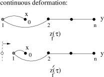
FIG. 2.: A folded trajectory at the end point of the path, and a similar one with $z_{1}$ closer to $z_{0}$.

We conclude that a calculation in quenched approximation, where the creation of particle-antiparticle pairs can only come from $Z$-graphs, must be more stable (produce a larger mass) than a similar calculation without any Z-graphs or $\chi\bar{\chi}$ pairs. The quenched $\chi^{2}\phi$ theory therefore is bounded by the same limits given in Eq. (46). This conclusion supports, and is supported by, the results of Refs. [2, 9, 10] which show, in the quenched approximation, that the $\chi^{2}\phi$ interaction is stable for a finite range of coupling strengths.

It is now clear that the instability of $\chi^{2}\phi$ theory must be due to either (i) the possibility of creating an infininte number of closed $\chi\bar{\chi}$ loops, or (ii) the presence of an infinite number of matter particles (as in an infinite medium). Indeed, the original proof given by Baym used the possibility of loop creation from the vacuum to prove that the vacuum was unstable. In fact, the FS representation can be used to show explicitly that the critical coupling $g^{2}_{\rm crit}$ decreases as $1/L$, where $L$ is the number of closed loops, in agreement with the estimate of Eq. (46)[11].

This work was supported in part by the US Department of Energy under grant No. DE-FG02-97ER41032. The Southeastern Universities Research Association (SURA) operates the Thomas Jefferson National Accelerator Facility under DOE contract DE-AC05-84ER40150.

REFERENCES

• [1] G. Baym, Phys.Β Rev.Β 117, 886 (1959).
• [2] Γ‡. ŞavklΔ±, J.Β A.Β Tjon, and F.Β Gross, Phys. Rev.Β C 60 055210 (1999).
• [3] R. Rosenfelder, A.W. Schreiber, Phys. Rev. D 53 3337, 1996; Phys. Rev. D53, 3354, 1996; hep-ph/9911484.
• [4] B.Β Ding and J.Β Darewych, J.Β Phys.Β G, 26, 907 (2000).
• [5] Yu. A. Simonov and J. A. Tjon, Ann. Phys. 228, 1 (1993).
• [6] T. Nieuwenhuis and J. A. Tjon, Phys. Rev. Lett. 77, 814 (1996).
• [7] T. Nieuwenhuis, PhD-thesis, University of Utrecht (1995), unpublished.
• [8] Γ‡. ŞavklΔ±, F.Β Gross, J.Β A.Β Tjon, Phys Review D 62 116006
• [9] Γ‡. ŞavklΔ± Oct 2000. 33pp. Lectures given at 13th Indian Summer School: Understanding the Structure of Hadrons, Prague, Czech Republic, 28 Aug - 1 Sep 2000. To be published in Czech.Β J.Β Phys, hep-ph/0011249
• [10] Γ‡. ŞavklΔ±, hep-ph/9910502, ( accepted for publication in Comp. Phys. Comm.)
• [11] Γ‡. ŞavklΔ±, F.Β Gross, and J.Β A.Β Tjon, in preparation.