How a quark-gluon plasma phase modifies the bounds on
extra dimensions from SN1987a

Abstract

The shape of the neutrino pulse from the supernova SN1987a provides one of the most stringent constraints on the size of large, compact, “gravity-only” extra dimensions. Previously, calculations have been carried out for a newly-born proto-neutron star with a temperature of about 50 MeV at nuclear matter density. It is arguable that, due to the extreme conditions in the interior of the star, matter might be a quark-gluon plasma, where the relevant degrees of freedom are quarks and gluons rather than nucleons. We consider an energy-loss scenario where seconds after rebounce the core of the star consists of a hot and dense quark-gluon plasma. Adopting a simplified model of the plasma we derive the necessary energy-loss formulae in the soft-radiation limit. The emissivity is found to be comparable to the one for nuclear matter and bounds on the radius of extra dimensions are similar to those found previously from nuclear matter calculations.

I Introduction

Ideas that we live in a world consisting of $d$ compact extra dimensions in addition to the usual four infinite dimensions are not new and date back to the 1930s. They imply that there are Kaluza-Klein (KK)-modes corresponding to excitations of ordinary standard model particles in the extra dimensions. Such modes, however, have not been seen in any collider experiment so far [1].

Recently, a variation of this concept has been revitalized by Arkani-Hamed et al. [2, 3, 4] who considered an alternative picture in which standard model fields are confined to a four-dimensional “brane” while gravity, constituting the dynamics of space-time itself, is allowed to propagate into the whole (4+$d$) dimensional “bulk”. This picture caused some excitement because it provides a natural solution to the hierarchy problem. As detailed in [3], the extension of the four-dimensional space for gravitons leads to a “dilution” of gravity into the extra dimensions and therefore to the smallness of Newton’s gravitational constant $G_{N}$. Matching the Planck mass $M_{\text{Pl}(4)}$ in the four-dimensional world to the one in the (4+$d$) dimensional world, $M_{\text{Pl}(4+d)}$, via the relation

$$M_{\text{Pl}(4)}^{2}\sim R^{d}M_{\text{Pl}(4+d)}^{2+d},$$ (1)

one can bring the Planck mass down from $10^{19}$ TeV to the weak scale of $~{}1$ TeV by choosing an appropriate size $R$ of the extra dimensions. For one extra dimension, $R\sim 10^{11}$ m, in this case gravity—specifically Newton’s inverse-square law—would be modified on the scale of astronomical distances, a case clearly ruled out. But already for $d=2$, $R\sim 1$ mm, which is just out of reach to present experimental measurements of the gravitational force law [6].

Another way of testing these models is to search for “beyond the standard model” physics at the scale $M_{\text{Pl}(4+d)}$. Even though one would naively expect a violation of the standard model at this scale to be of only gravitational strength, the large number of excited KK-modes at such high energies compensates for the weak coupling between these KK-modes and the ordinary matter fields. Such effects could alter standard model predictions due to virtual KK-mode contributions or manifest themselves in the form of massive graviton production [7, 8, 9]. It might be possible that such effects can be seen in the form of missing energy at future colliders operating at the TeV scale like the CERN LHC [10, 11].

The most stringent constraints on the size of extra dimensions come from astrophysical considerations. Recently it has been pointed out that an overproduction of massive KK modes in the early universe might result in early matter domination and therefore a lower age of the universe [12].

Another way to obtain bounds on the size of extra dimensions from astrophysics comes from supernova SN1987a. Our current theory of supernovae predicts the shape and duration of SN1987a’s neutrino pulse very well. Hence, if some new channel transports too much energy from the interior of the supernova then the current understanding of SN1987a’s neutrino signal gets invalidated. Raffelt [13] has quantified the maximum possible emissivity for a new energy loss process which doesn’t conflict with our current understanding of the neutrino signal as $10^{19}$ ergs/g/s. Using this criteria there have been several calculations [14, 15, 16] to obtain bounds on the size of the extra dimensions for a newly born proto-neutron star assuming that the interior of the star consists of nuclear matter at a temperature of $\sim 50$ MeV. A more rigorous approach has been undertaken recently by Hanhart et al. [17] who performed detailed simulations of the effect of exotic radiation on the neutrino signal.

Although the star’s inner core might well consist of nuclear matter, because of the extreme conditions seconds after core bounce with a density in some regions possibly up to $\sim 15$ times the nuclear matter density $n_{0}=0.17~{}\text{fm}^{-3}$ and a temperature of maybe up to $\sim 100$ MeV, matter is near a phase transition to a deconfined QCD plasma.

It is therefore important to investigate how bounds on the size of extra dimensions change if a scenario is considered where, in contrast to taking nucleons as the relevant degrees of freedom, the calculation is carried out using quarks and gluons as degrees of freedom. However, in the regime we are considering here matter is not in a state where the density and temperature are so high that a first order perturbative calculation would suffice; it is rather in a regime where deconfinement just sets in and the QCD coupling constant is still large (${\alpha}_{s}\sim 1$). For this reason we will carry out our calculations for a (unphysical) regime of very high density (up to $10^{7}n_{0}$). There, the coupling is weak and perturbative calculations are feasible. From there we extrapolate down to get the emissivity in the physical region.

Note that if the temperature falls below a critical temperature $T_{c}$ of $\sim 50$ MeV (for a density of a few times nuclear density) this very dense plasma most likely undergoes a phase-transition to a color superconducting phase (for a recent review see [18]). Since we do not consider such a scenario here, we assume the temperature to be above $T_{c}$.

The paper is organized as follows: In Section II we calculate the amplitude for the emission of soft gravi- and dilastrahlung into KK-modes from quark-quark (qq) scattering in a degenerate QCD plasma. This calculation is fairly general, it applies to soft radiation of KK-modes from light relativistic fermions. Then, in Section III, we consider a simple model of the plasma consisting of three light quark flavors to estimate the size of the qq scattering cross sections. To treat the occurring divergences for colinear scattering we incorporate the effects of the surrounding plasma into the gluon propagator by introducing a cutoff mass. We do not consider any other many-body effects; our goal is to obtain an estimate for the qq scattering cross section, an exact calculation is presently not feasible. In Section IV, we carry out the phase-space integration to get a formula for numerical calculation of the emissivity of a gas of weakly interacting quarks. We also provide an approximation formula for the degenerate limit. Finally, in Section V, we calculate the emissivity and the bounds on the size of the $d$ extra dimensions for the case of $d=2$ and $d=3$ and compare them to the result from previous nuclear matter calculations.

II 4D-Graviton, KK-Graviton, and KK-Dilaton Radiation from Quark-Quark Scattering

We assume the $d$ extra dimensions to form a $d$-torus with radius $R$ so that the KK-graviton and KK-dilation mode expansions are given by

$$h^{\mu\nu}(x,y)=\sum_{\vec{j}}h^{\mu\nu,\vec{j}}(x)\exp\left(i\frac{\vec{j}\cdot\vec{y}}{R}\right)\quad\text{and}\quad\phi_{ab}(x,y)=\sum_{\vec{j}}h_{ab}^{\vec{j}}(x)\exp\left(i\frac{\vec{j}\cdot\vec{y}}{R}\right),$$ (2)

respectively. In addition to these particles there emerge massive spin-1 particles from the KK reduction of the Fierz-Pauli Lagrangian [7] which decouple from matter and need not be considered here.

The coupling of the 4D-graviton $g\equiv h$, KK-graviton $h^{\vec{j}}$, and KK-dilaton $\phi^{\vec{j}}$ to the energy-momentum tensor $T_{\mu\nu}$ of the matter field is governed by the Lagrange density

$${\cal L}=-\frac{\kappa}{2}\left(h^{\mu\nu}T_{\mu\nu}+\sum_{\vec{j}}\left[h^{\mu\nu,\vec{j}}T_{\mu\nu}+\sqrt{\frac{2}{3(d+2)}}\phi_{aa}^{\vec{j}}T^{\mu}_{\mu}\right]\right),$$ (3)

where $\kappa$ is defined as $\kappa=\sqrt{16\pi G_{N}}$ with $G_{N}$ being Newton’s gravitational constant. Note that in Eq. (3) the massless graviton $h_{\mu\nu}$—being the zero-mode of the $h^{\mu\nu,\vec{j}}$ modes—has been written separately for clarity. The energy-momentum tensor $T_{\mu\nu}$ for a free quark is given by

$$T_{\mu\nu}=\frac{i}{2}\bar{\psi}\left(\overrightarrow{\partial_{\mu}}-\overleftarrow{\partial_{\mu}}\right)\gamma_{\nu}\psi-g_{\mu\nu}\left[\frac{i}{2}\bar{\psi}\gamma^{\alpha}(\overrightarrow{\partial_{\alpha}}-\overleftarrow{\partial_{\alpha}})\psi-m\bar{\psi}\psi\right].$$ (4)

As we will discuss in the next section, the leading contribution from gravitational emission for the degenerate quark-gluon plasma of our model comes from the qq scattering processes $qq\rightarrow qqX$, where a low-momentum 4D-graviton ($X=g$), KK-graviton ($X=h$), or KK-dilaton ($X=\phi$) is emitted.

A Amplitude for $qq\rightarrow qqX$ in the Soft Limit

For a degenerate plasma the participating quarks are near the Fermi surface and hence the momentum $\vec{k}$ of the emitted graviton is small compared to the quark momenta. In the soft limit the leading diagrams for the process $qq\rightarrow qqX$ are those where the graviton radiates off one of the external legs as shown in Fig. 1 (bremsstrahlung process).

FIG. 1.: The leading order diagrams for the process $qq\rightarrow qqX$. In the soft limit these diagrams are dominant over those where the graviton couples to some internal line. ${\cal A}$ is the on-shell amplitude for quark-quark scattering.

For small $\vec{k}$ these diagrams are ${\cal O}(k^{-1})$ while diagrams where the graviton couples to some internal line are ${\cal O}(1)$ and therefore suppressed [20, 21, 22].

The amplitude $M_{\mu\nu}$ of this process then factorizes into the amplitude ${\cal A}$ (which includes a sum over spins and colors of the incoming and outgoing quarks) for on-shell $qq\rightarrow qq$ scattering and the conserved gravitational current $T_{\mu\nu}$. To lowest order in $\vec{k}$, $M_{\mu\nu}$ can be written as [16]

$$M_{\mu\nu}=\frac{\kappa}{2}\sum_{j=1}^{4}\eta_{j}{p_{j}}_{\mu}{p_{j}}_{\nu}\frac{1}{p_{j}\cdot k}\,{\cal A},$$ (5)

where

$$\eta_{j}=\left\{\begin{array}[]{cl}1&\text{if }j=1,2\\ -1&\text{if }j=3,4\end{array}\right.\\ .$$ (6)

Here, the $p_{j}$ denote the four-momenta of the incoming ($j=1,2$) and outgoing ($j=3,4$) quarks while $k=({\omega},\vec{k})$ is the graviton’s four-momentum. The result Eq. (5) has been calculated by Weinberg [23] using an entirely classical derivation. This is not unexpected since to lowest order in $\vec{k}$ graphs where the radiation comes from an internal line are suppressed and so the radiation from the external legs is the dominant one, corresponding to classical bremsstrahlung from the gravitational charges accelerated during the collision.

B Energy-Loss Formulae

The energy loss into a KK-mode $\vec{j}$ and into the momentum space volume element $d^{3}k$ due to 4D-graviton, KK-graviton, and KK-dilation emission is given by

$$d\epsilon_{g}=\omega\frac{d^{3}k}{(2\pi)^{3}2\omega}\sum_{\lambda}\left[M^{{\alpha}\beta}\epsilon_{{\alpha}\beta}(\vec{k},\lambda)\right]^{*}M^{\mu\nu}\epsilon_{\mu\nu}(\vec{k},\lambda)=\omega\frac{d^{3}k}{(2\pi)^{3}2\omega}\left({M^{\lambda\nu}}^{*}M_{\lambda\nu}-\frac{1}{2}\left|M^{\lambda}_{\phantom{\lambda}\lambda}\right|^{2}\right),$$ (7)

$$d\epsilon^{\vec{j}}_{h}=\omega\frac{d^{3}k}{(2\pi)^{3}2\omega}\sum_{\lambda=1}^{5}\left[M^{{\alpha}\beta}\epsilon^{\vec{j}}_{{\alpha}\beta}(\vec{k},\lambda)\right]^{*}{M^{\mu\nu}\epsilon^{\vec{j}}_{\mu\nu}(\vec{k},\lambda)},$$ (8)

and

$$d\epsilon^{\vec{j}}_{\phi}=\frac{2}{3(d+2)}\omega\frac{d^{3}k}{(2\pi)^{3}2\omega}M_{\alpha}^{\phantom{{\alpha}}{\alpha}}M_{\beta}^{\phantom{\beta}\beta}\sum_{\lambda=1}^{n(n-1)/2}\left[e^{\vec{j}}_{ii}(\vec{k},\lambda)\right]^{*}e^{\vec{j}}_{jj}(\vec{k},\lambda)=\frac{d^{3}k}{2(2\pi)^{3}}M_{\alpha}^{\phantom{{\alpha}}{\alpha}}M_{\beta}^{\phantom{\beta}\beta}\frac{2(d-1)}{3(d+2)},$$ (9)

respectively. Here, $\epsilon_{\mu\nu}$, $\epsilon^{\vec{j}}_{\mu\nu}$, and $e^{\vec{j}}_{\mu\nu}$ are the polarization tensors of the 4D-graviton, KK-graviton, and KK-dilaton, respectively [7].

Utilizing the conservation of the energy-momentum tensor, $k^{\mu}M_{\mu\nu}=0$, $M_{\mu\nu}$ can be expressed in terms of the purely spacelike components as

$$M_{0i}=-\frac{k^{j}}{\omega}M_{ji},\quad M_{00}=\frac{k^{i}k^{j}}{\omega^{2}}M_{ji}$$ (10)

or, upon defining

$$W_{\mu\nu ij}=\eta_{i\mu}\eta_{j\nu}-\eta_{i\mu}\eta_{0\nu}\frac{k_{j}}{\omega}-\eta_{0\mu}\eta_{j\nu}\frac{k_{i}}{\omega}+\eta_{0\mu}\eta_{0\nu}\frac{k_{i}k_{j}}{\omega^{2}},$$ (11)

be written as

$$M_{\mu\nu}=W_{\mu\nu ij}M^{ij}.$$ (12)

Using this notation the energy loss formulae in Eqs. (7)–(9) can be written solely in terms of the space-space components of the tensor $M_{\mu\nu}$ as

$$d\epsilon^{\vec{j}}_{X}=\frac{dkk^{2}}{4\pi^{2}}\frac{d\hat{k}}{4\pi}M_{ij}\Lambda_{X}^{ijkl}M_{kl},$$ (13)

where the $\Lambda_{X}^{ijkl}$ are given by

$$\Lambda_{g}^{ijkl}=\delta^{ik}\delta^{jl}-\frac{1}{2}\delta^{ij}\delta^{kl}-\frac{1}{2k^{2}}\left(4k^{j}k^{l}\delta^{ik}-k^{k}k^{l}\delta^{ij}-k^{i}k^{j}\delta^{kl}\right)+\frac{1}{2k^{4}}k^{i}k^{j}k^{k}k^{l},$$ (14)

$$\Lambda_{h}^{ijkl} = W^{\mu\nu ij}B_{\mu\nu{\alpha}\beta}W^{{\alpha}\beta kl}$$ (15)

$$= \left(\delta^{ik}\delta^{jl}+\delta^{il}\delta^{jk}-\frac{2}{3}\delta^{ij}\delta^{kl}\right)+\frac{4}{3\omega^{4}}k^{i}k^{j}k^{k}k^{l}$$ (17)

$$-\frac{1}{\omega^{2}}\left(\delta^{ik}k^{j}k^{l}+\delta^{jk}k^{i}k^{l}+\delta^{il}k^{j}k^{k}+\delta^{jl}k^{i}k^{k}-\frac{2}{3}(k^{i}k^{j}\delta^{kl}+k^{k}k^{l}\delta^{ij})\right),$$

and

$$\Lambda_{\phi}^{ijkl}=W_{{\alpha}\phantom{{\alpha}}}^{\phantom{{\alpha}}{\alpha}ij}W_{\beta\phantom{\beta}}^{\phantom{\beta}\beta kl}\frac{2(d-1)}{3(d+2)}=\left(\delta^{ij}\delta^{kl}+\frac{1}{\omega^{2}}\left[\delta^{ij}k^{k}k^{l}+\delta^{kl}k^{i}k^{j}\right]+\frac{1}{\omega^{4}}k^{i}k^{j}k^{k}k^{l}\right)\frac{2(d-1)}{3(d+2)}.$$ (18)

The tensor $B_{\mu\nu{\alpha}\beta}$, defined by the spin sum of the KK-graviton polarization tensors

$$\sum_{{\lambda}=1}^{5}\epsilon_{\mu\nu}^{\vec{j}}(\vec{k},{\lambda})\left[\epsilon_{\rho\sigma}^{\vec{j}}(\vec{k},{\lambda})\right]^{*}=B_{\mu\nu\rho\sigma}^{\vec{j}}(\vec{k}),$$ (19)

is given in [7, 8].

We will now choose the center-of-momentum (COM) frame as our reference frame where the 4-momenta of the two incoming quarks are given by $(p^{0},\vec{p})$ and $(p^{0},-\vec{p})$ and those of the outgoing quarks by $({p^{\prime}}^{0},\vec{p^{\prime}})$ and $({p^{\prime}}^{0},-\vec{p^{\prime}})$. The COM scattering angle ${\theta_{\text{cm}}}$ is defined by $\vec{p}\cdot\vec{p^{\prime}}=pp^{\prime}\cos{{\theta_{\text{cm}}}}$. We also assume the quarks to have equal mass.

If the momenta of the scattering particles are much smaller than their rest mass $M$—as is the case in soft radiation from nucleon-nucleon scattering—it can be neglected in the denominator in Eq. (5) and $M_{\mu\nu}$ is simply given by [16]

$$M_{ij}=\frac{{\kappa}}{M{\omega}}\left(p_{i}p_{j}-p^{\prime}_{i}p^{\prime}_{j}\right)\,{\cal A}.$$ (20)

In our case, however, this approximation is inappropriate since the quark mass is very small compared to the quark Fermi momenta, we therefore write Eq. (5) as

$$M_{ij}=\frac{\kappa}{2}\left(\frac{p_{i}p_{j}}{p^{0}\omega-\vec{p}\cdot\vec{k}}+\frac{p_{i}p_{j}}{p^{0}\omega+\vec{p}\cdot\vec{k}}-\frac{p^{\prime}_{i}p^{\prime}_{j}}{p^{\prime 0}\omega-\vec{p^{\prime}}\cdot\vec{k}}-\frac{p^{\prime}_{i}p^{\prime}_{j}}{p^{\prime 0}\omega+\vec{p^{\prime}}\cdot\vec{k}}\right){\cal A}.$$ (21)

The $\int{d\hat{k}}/{4\pi}$ integration in Eq. (13) can then be carried out analytically for the three cases. For soft graviton radiation the quark momenta are assumed to lie on the Fermi surface and it is justified to assume $|\vec{p}|\approx|\vec{p^{\prime}}|$. We can then approximate the momenta $p$ and $p^{\prime}$ by

$$\bar{p}^{2}=\frac{p^{2}+{p^{\prime}}^{2}}{2}.$$ (22)

Replacing $p$ and $p^{\prime}$ with $\bar{p}$ the formulae simplify considerably and the $\int{d\hat{k}}/{4\pi}$ integration can be written as

$$\int\frac{d\hat{k}}{4\pi}M_{ij}\Lambda_{X}^{ijkl}M_{kl}=\frac{{\kappa}^{2}\bar{p}^{2}}{{\omega}k}g_{X}(x,y,{\theta_{\text{cm}}})\left|{\cal A}\right|^{2}$$ (23)

in terms of ${\cal A}$ and the dimensionless functions $g_{X}$ which are given in the Appendix. Here we have also defined $x=m_{\vec{j}}/{\omega}$ and $y={\bar{p}}^{0}/\bar{p}={\sqrt{{\bar{p}}^{2}+M^{2}}}/\bar{p}$.

Note that for massless quarks one of the denominators in Eq. (21) becomes zero if the momentum of that quark is parallel to $\vec{k}$ and one might think that this term becomes infinite. However, as already noted in Ref. [23] for the case of the massless 4D-graviton, this singularity is only spurious and gets canceled by $\Lambda_{X}^{ijkl}$ in the numerator so that $g_{X}$ is finite not only for $X=g$, but also for $X=h$ and $X=\phi$.

We can then employ the energy-momentum relation for the KK-mode $\vec{j}$ and write the formula for the energy loss per unit frequency interval into the given KK-mode of mass $m_{\vec{j}}^{2}={\omega}^{2}-k^{2}$ as

$$\frac{d\epsilon_{X}^{\vec{j}}}{d{\omega}}=\frac{{\omega}k}{4\pi^{2}}\int\frac{d\hat{k}}{4\pi}M_{ij}\Lambda_{X}^{ijkl}M_{kl}=\frac{{\kappa}^{2}\bar{p}^{2}}{4\pi^{2}}g_{X}(x,y,{\theta_{\text{cm}}})\left|{\cal A}\right|^{2}.$$ (24)

This result is general as it applies to soft radiation from any light relativistic fermions with equal mass, not just to the quarks we are about to consider.

III A Simple Plasma Model

After bounce the homologous core of the star undergoing a supernova explosion gets compressed to a very high density. Previous calculations [14, 15, 16] assumed a density of $1-3$ times nuclear matter density $n_{0}=0.17$ fm and a temperature of $T\approx 30-80$ MeV corresponding to a (non-relativistic) nucleon chemical potential of $\mu_{N}\approx 50-100$ MeV.

Under such extreme conditions the star’s core not only consists of free neutrons and protons but these degrees of freedom are highly excited and near a phase transition to a deconfined quark-gluon plasma. It is therefore worthwhile to investigate how the graviton emissivity and hence the bounds on extra dimensions change if one carries out the calculations in this regime. Our intention here is to investigate graviton radiation into extra dimension from such a QCD plasma.

The physics of a QCD plasma under such violent conditions is particularly rich. In addition to quarks of different flavors, a variety of other particles are present and being produced constantly, such as electrons, positrons, neutrinos, and collective excitations like plasmons. The properties of the quark-gluon plasma are far from being completely understood so that we do not even attempt to take the whole richness of matter under such extreme conditions into account here. Instead, we assume a rather simply model for the plasma (not unlike the one used in Ref. [24]) where, in addition to electrons and neutrinos, only $u$, $d$, and $s$ quarks are assumed to be present. The possible weak reactions in the plasma are then

$$d\leftrightarrow u+e^{-}+{\nu}_{e}^{-}\quad\text{and}\quad s\leftrightarrow u+e^{-}+{\nu}_{e}^{-}.$$ (25)

At thermal equilibrium the chemical potentials have to add up to zero. For a low temperature $T$ this requirement reads

$${\mu}_{d}={\mu}_{u}+{\mu}_{e}+{\mu}_{\nu}\quad\text{and}\quad{\mu}_{s}={\mu}_{u}+{\mu}_{e}+{\mu}_{\nu}.$$ (26)

In addition, we want to satisfy charge neutrality, thereby imposing the constraint

$$0=Q=\frac{2}{3}n_{u}-\frac{1}{3}n_{d}-\frac{1}{3}n_{s}-n_{e}.$$ (27)

These three conditions can be simultaneously satisfied by choosing

$$n_{u}=n_{d}=n_{s}=\frac{n_{q}}{3}=n_{B}\quad\text{and}\quad n_{e}=n_{\nu}=0,$$ (28)

where $n_{q}$ is the quark number density and $n_{B}$ denotes the baryon number density. We do not consider dynamical production of these or any heavier quark flavors. As an additional simplification we take the mass of the $u$, $d$, and $s$ quarks to be zero.

The main contribution to graviton radiation from this plasma comes from the bremsstrahlung reaction $qq\rightarrow qqX$ ($X=g,h,\phi$) where a graviton is radiated from an external quark leg. This reaction is of order ${\cal O}({\kappa}{\alpha}_{s})$ where ${\alpha}_{s}$ is the QCD coupling constant. As we will see below, ${\alpha}_{s}$ is rather large and ${\cal O}(1)$. Moreover, we get contributions from processes involving dynamical produced electrons ($e$) and positrons ($p$), like $ee\rightarrow eeX$ or $ep\rightarrow epX$. These reactions are suppressed compared to $qq\rightarrow qqX$ by a factor of ${\alpha}_{\text{QED}}/{\alpha}_{s}$, where ${\alpha}_{\text{QED}}=1/137$ is the fine-structure constant. More contributions come from graviton-production reactions like $q\rightarrow qXX$. These, however, are ${\cal O}({\kappa}^{2})$ and therefore highly suppressed. We also assume that because of $T\ll\mu_{q}$ the number density of gluons is much smaller than that of quarks and therefore we do not consider the reaction $qg\rightarrow qX$. Note that the inclusion of any KK-modes generated by channels we neglect will only increase the emissivity and strengthen the bounds obtained below.

The baryon number density $n_{B}$ in the central core region of a stable neutron star is $\sim 1-15$ times the nuclear matter density $n_{0}=0.17~{}\text{fm}^{-3}$, depending on the nuclear matter equation of state used (compare Ref. [24] and values cited therein). Assuming quark matter, the (relativistic) quark chemical potential $\mu_{q}$ can be related to the quark density $n_{q}$ using the formula

$$n_{q}=6\frac{1}{2\pi^{2}}\int_{0}^{\infty}d{\epsilon}\,{\epsilon}^{2}N_{q}({\epsilon})$$ (29)

where $N_{q}({\epsilon})=(\exp[({\epsilon}-\mu_{q})/T]+1)^{-1}$ is the mean occupation number and ${\epsilon}$ is the (relativistic) quark energy. Choosing $n_{q}$ and $T$ we can then determine $\mu_{q}$; for $T=50$ MeV and $n_{q}=10-20n_{0}$ we find $\mu_{q}\approx 500-600$ MeV, which is in good agreement with other calculations [24]. Therefore quark matter has $\mu_{q}/T\gg 1$ which confirms our assumption that it is degenerate.

Furthermore, using $\mu_{q}$ and $T$ we can calculate the average momentum square $\langle p^{2}\rangle$ carried by the quarks using

$$\langle p^{2}\rangle=\frac{\int d^{3}p\,p^{2}N_{q}({\epsilon})}{\int d^{3}p\,N_{q}({\epsilon})}.$$ (30)

For typical parameters for the plasma ($n_{q}\approx 10-20n_{0}$, $T\approx 50$ MeV) we calculate the average momentum carried by the quarks to be $p\approx 420-520$ MeV which is just about the order of energy at which the strong interaction becomes strong and the QCD coupling constant ${\alpha}_{s}$ is expected to be rather large. Of course, this is eventually a sign that matter under these conditions is at the phase transition to the QCD phase. Therefore this regime is particularly difficult to treat because on the one hand nucleonic degrees of freedom are no longer the proper degrees of freedom while on the other hand perturbative QCD calculations are notoriously difficult.

For this reason we will evaluate the emissivity for unphysically high densities of $n_{q}\sim 100-10^{7}n_{0}$ and extrapolate from this region down to the physical regime. At such high densities the momentum carried by the quarks is $p\sim 1-40$ GeV. This being in the perturbative regime, we can estimate the strength of the QCD coupling constant ${\alpha}_{s}$ employing the leading-log formula for the running coupling [derived from the ${\beta}$-function to ${\cal O}({\alpha}_{s}^{2})$]

$${\alpha}_{s}=\frac{g^{2}}{4\pi}=\frac{12\pi}{(33-2N_{F})\ln\frac{\langle p^{2}\rangle}{\Lambda^{2}}}$$ (31)

which gives ${\alpha}_{s}\approx 0.48-0.13$—small enough for perturbative calculations. To check the effects of higher order correction we also use the formula

$${\alpha}_{s}=\frac{g^{2}}{4\pi}=\frac{4\pi}{{\beta}_{0}u}\left(1-\frac{2{\beta}_{1}}{{\beta}_{0}^{2}}\frac{\ln u}{u}+\frac{4{\beta}_{1}^{2}}{{\beta}_{0}^{4}\ln^{2}u}\left[\left(\ln u-\frac{1}{2}\right)^{2}+\frac{{\beta}_{2}{\beta}_{0}}{8{\beta}_{1}^{2}}-\frac{5}{4}\right]\right)$$ (32)

derived from the ${\beta}$-function to 4th order in ${\alpha}_{s}$. Here

$${\beta}_{0}=11-\frac{2}{3}N_{F},\quad{\beta}_{1}=51-\frac{19}{3}N_{F},\quad{\beta}_{2}=2857-\frac{5033}{9}N_{F}+\frac{325}{27}N_{F}^{2},\text{ and }u=\ln\frac{\langle p^{2}\rangle}{\Lambda^{2}},$$ (33)

where $\Lambda\approx 200$ MeV is taken as the QCD breakdown scale and $N_{F}=3$ is the number of flavors. The formula in Eq. (32) changes ${\alpha}_{s}$ by about $18-37\%$ compared to Eq. (31).

It is instructive to compare the number of nucleons $N_{N}$ and quarks $N_{q}$ participating in scattering for the two cases of nucleon-nucleon scattering (for simplicity we assume here neutron matter) and qq scattering in the degenerate limit. For low temperature the baryon number density $n_{B}$ is approximately proportional to $p_{F}^{3}$. For nucleons $n_{B}\approx p_{F}^{3}/(3\pi^{2})$, while for quarks $n_{B}\approx p_{F}^{3}/\pi^{2}$. The number of particles $N_{N}$ [$N_{q}$] participating in scattering is roughly proportional to the momentum-space volume of a shell of the Fermi sphere with radius $p_{F}$ and thickness $dE\approx T$ leading to $N_{N}\approx 8\pi p_{F}^{2}\,dp$ [$N_{q}\approx 72\pi p_{F}^{2}\,dp$] in the nucleon [quark] case. Making use of the energy-momentum relations $p\,dp=M\,dE$ [$p\,dp=p\,dE$] this becomes $N_{N}\approx\pi(3\pi^{5})^{1/3}n_{B}^{1/3}MT$ [$N_{q}=72\pi^{7/3}n_{B}^{2/3}T$]. Using $M\approx 940$ MeV the ratio of $N_{N}$ and $N_{q}$ for a density of $n_{B}=10n_{0}$ is

$$\frac{N_{N}}{N_{q}}\approx 0.3$$ (34)

and hence, despite the fact that the quarks have a higher number of degrees of freedom, the number of particles participating in scattering is not much different in the two cases.

A Quark-Quark Scattering Cross Sections

The matrix elements for the scattering of quarks to first order in ${\alpha}_{s}$ can be calculated from the one-gluon exchange diagrams and are given in [25]. For quarks of different flavor the squared matrix element can be written as

$$\left|{\cal A}_{qq^{\prime}}\right|^{2}=256\pi^{2}{\alpha}_{s}^{2}\frac{s^{2}+u^{2}}{t^{2}}$$ (35)

and for quarks of the same flavor as

$$\left|{\cal A}_{qq}\right|^{2}=256\pi^{2}{\alpha}_{s}^{2}\left(\frac{s^{2}+u^{2}}{t^{2}}+\frac{s^{2}+t^{2}}{u^{2}}-\frac{2}{3}\frac{s^{2}}{ut}\right)$$ (36)

(see Fig. 2).

FIG. 2.: The lowest order diagrams for scattering of quarks of the same flavor.

Here $s$, $t$, and $u$ are the usual Mandelstam variables given in the COM frame for zero quark mass by $s=4p^{2}=4{p^{\prime}}^{2}$, $t=-2p^{2}(1-\cos{\theta_{\text{cm}}})$, and $u=-2p^{2}(1+\cos{\theta_{\text{cm}}})$, where ${\theta_{\text{cm}}}$ is the COM scattering angle.

Note that similar diagrams exchanging a photon instead of a gluon are suppressed by a factor of ${\alpha}_{\text{QED}}/{\alpha}_{s}$ and need not be considered.

The matrix elements in Eqs. (35) and (36) can become highly singular because of the $t^{2}$ and $u^{2}$ in the denominators. The momentum $q$ transfered by the exchanged gluon vanishes as ${\theta_{\text{cm}}}\rightarrow 0$ or ${\theta_{\text{cm}}}\rightarrow\pi$, which corresponds to colinear scattering. On the other hand, the energy-momentum tensor $M_{\mu\nu}$ also vanishes for colinear scattering and one might think that this would render the singularity spurious. However, this is not the case. An analysis of the functions $g_{X}$ shows that for ${\theta_{\text{cm}}}\approx 0$ [${\theta_{\text{cm}}}\approx\pi$] $g_{X}$ behaves like $\sim{\theta_{\text{cm}}}^{2}$ [$\sim(\pi-{\theta_{\text{cm}}})^{2}$] while $\left|{\cal A}_{qq}\right|^{2}$ and $\left|{\cal A}_{qq^{\prime}}\right|^{2}$ behave like $\sim 1/{\theta_{\text{cm}}}^{4}$ [$\sim 1/(\pi-{\theta_{\text{cm}}})^{4}$].

B Curing the Divergences

In the case of electron-electron scattering in an electron gas the divergences that one encounters are of a similar origin and are usually taken care of by including effects which screen the bare particles arising from the interaction of the electrons and photons with the surrounding matter. We will employ, without justification, a similar procedure in the present case of a QCD plasma.

The bare gluon propagator $D_{\mu\nu}$ is related to the gluon self-energy $\Pi_{\mu\nu}$ by Dyson’s equation

$$D_{\mu\nu}^{-1}=g_{\mu\nu}({\omega}^{2}-q^{2})+\Pi_{\mu\nu}.$$ (37)

Following Ref. [26], the matrix element for scattering of like quarks for small momentum transfer is equal to the one for unlike quarks and can be written as

$$\left|{\cal A}_{qq^{\prime}}\right|^{2}=128\pi^{2}{\alpha}_{s}^{2}\left|\frac{1}{q^{2}+\Pi_{l}^{2}}-\frac{(1-x^{2})\cos{\phi}}{q^{2}-{\omega}^{2}+\Pi_{t}}\right|^{2},$$ (38)

where $\Pi_{l}$ and $\Pi_{t}$ are the longitudinal and transverse gluon polarization functions given for $q\ll\mu_{q}$ by

$$\Pi_{l}=q_{D}^{2}\left(1-\frac{x}{2}\ln{\frac{x+1}{x-1}}\right)\quad\text{and}\quad\Pi_{t}=q_{D}^{2}\left(\frac{x^{2}}{2}+\frac{x(1-x^{2})}{4}\ln{\frac{x+1}{x-1}}\right).$$ (39)

Here $x={\omega}/q$ and $q_{D}$ is the Debye wave number for cold quark matter of three flavors given by $q_{D}^{2}=6{\alpha}_{s}\mu_{q}^{2}/\pi^{2}$. Note that for quarks of equal mass in the COM frame ${\omega}=0$ and therefore $\Pi_{t}=0$; the transverse part of the propagator is still unscreened, at least for $\Pi_{t}$ calculated to zeroth order in $x$. Since $T\ll\mu$ the participating quark’s momenta are near the Fermi surface and hence ${\omega}\simeq 0$, independent of the chosen reference frame. The problem of an unscreened transverse gluon propagator can be solved in some cases by retaining ${\cal O}(x)$ terms in Eq. (39) and is related to frequency-dependent screening [27].

Because of these complications we adopt here a much simpler method to incorporate the complicated screening effects. We will render the amplitudes in Eqs. (35) and (36) finite by including a Debye screening mass $m_{D}$, by substituting

$$t\rightarrow t-m_{D}^{2}\quad\text{and}\quad u\rightarrow u-m_{D}^{2}$$ (40)

for $u$ and $t$ in the denominator. For a small coupling constant the Debye mass to lowest order is given by

$$m_{D}^{2}=g^{2}\left(\frac{3}{2}T^{2}+\frac{1}{2\pi^{2}}\sum_{f}{\mu_{f}^{2}}\right)$$ (41)

which makes it about $60-20\%$ of a typical momentum transfer for densities $n_{q}=100-10^{7}n_{0}$. To consider higher order corrections to $m_{D}$ and to account for other many-body effects in the QCD plasma at these high densities we carry out the calculation for the emissivity not only using the value $m_{D}$ from Eq. (41) but also the values $m_{D}/3$ and $3m_{D}$, thereby spanning about an order of magnitude in the cutoff mass. As an example we show in Fig. 3

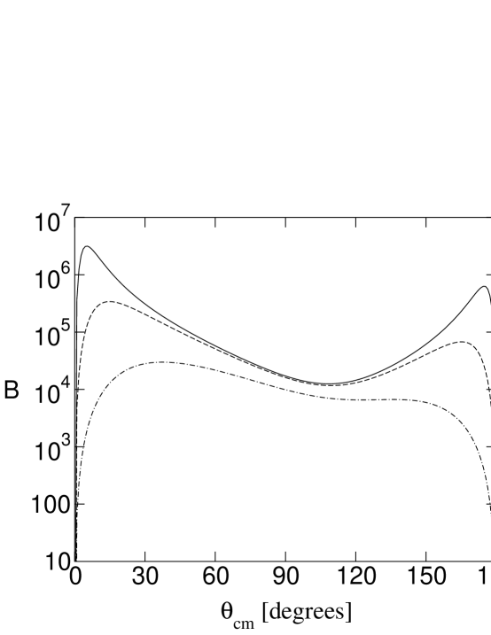
FIG. 3.: The function $B({\theta_{\text{cm}}})$ for $n_{q}=10^{5}n_{0}$ and for different cutoff masses $m_{D}/3$ MeV (solid line), $m_{D}$ MeV (dashed line), and $3m_{D}$ MeV (dot-dashed line) with $m_{D}=2250$ MeV. The typical COM momentum is 8400 MeV and ${\alpha}_{s}$ is set to 1.

the dimensionless function $B({\theta_{\text{cm}}})$ defined by

$$B({\theta_{\text{cm}}})=\left(\left|{\cal A}_{qq^{\prime}}\right|^{2}+\frac{\left|{\cal A}_{qq}\right|^{2}}{4}\right)\sin^{2}{{\theta_{\text{cm}}}},$$ (42)

which enters the formula for the emissivity for a varying cutoff mass $m_{D}$. The factor $\sin^{2}{{\theta_{\text{cm}}}}$ in $B({\theta_{\text{cm}}})$ is an approximation for $\int_{0}^{1}dx\,x^{d-1}g_{X}(x,1,{\theta_{\text{cm}}})$ as explained in the next section. $B({\theta_{\text{cm}}})$ has been calculated for a plasma at the density $n_{q}=10^{5}n_{0}$ where a typical COM momentum is about 8400 MeV and $m_{D}\approx 2250~{}MeV$. The variation of $m_{D}$ of about one order of magnitude causes a variation in $B({\theta_{\text{cm}}})$ of about 1-2 orders of magnitude.

Other possible ways to regulate these divergences could be to introduce a cutoff of order $m_{D}$ for the gluon-momentum integration or to cut off the integration over ${\theta_{\text{cm}}}$ at some small angle $1/\Lambda$ when calculating observables. The latter technique was used by Weinberg [23] to calculate the power produced in gravitational radiation from the hydrogen plasma in the sun.

IV Gravitational Emissivity of a Gas of Relativistic Fermions

In order to calculate the emissivity due to graviton radiation from the two-body scattering reaction $qq\rightarrow qqX$ in a gas of relativistic quarks we have to integrate over the phase space of incoming ($\vec{p_{1}}$, $\vec{p_{2}}$) and outgoing ($\vec{p^{\prime}_{1}}$, $\vec{p^{\prime}_{2}}$) quarks as well as that of the emitted gravitational particle ($\vec{k}$). The formula for the emissivity is then given by

$$\frac{d{\cal E}_{X}}{dt} = \sum_{\vec{j}}\int d{\omega}\int\left[\prod_{i=1..2}\frac{d^{3}p_{i}}{(2\pi)^{3}2E_{i}}\frac{d^{3}p_{i}^{\prime}}{(2\pi)^{3}2E^{\prime}_{i}}\right]f_{1}f_{2}(1-f_{1}^{\prime})(1-f_{2}^{\prime})$$ (44)

$$\times(2\pi)^{4}\delta^{4}(p_{1}+p_{2}-p_{1}^{\prime}-p_{2}^{\prime}-k)\frac{d{\epsilon}_{X}^{\vec{j}}}{d{\omega}}.$$

Here, again, the $X$ stands for the type of gravitational radiation, massless 4D-gravitons ($X=g$), massive KK-gravitons($X=h$), or massive KK-dilatons ($X=\phi$). The functions $f$ are Pauli blocking factors given by $f_{i}=(\exp[(E_{i}-{\mu})/T]+1)^{-1}$, furthermore $E_{i}=\left|\vec{p_{i}}\right|$ for massless quarks. The summation over the KK-modes $\vec{j}$ doesn’t apply to the massless 4D-graviton, obviously.

This formula applies for scattering of differently flavored quarks. A symmetry factor of $1/4$ would have to be included for scattering of quarks having the same flavor to account for identical particles in the initial and final states. We will consider this symmetry factor at the beginning of the next section.

In the soft-radiation limit we can neglect the graviton momentum $\vec{k}$ in the momentum-conserving delta function. Furthermore, by introducing the total momentum $\vec{P}=\vec{p_{1}}+\vec{p_{2}}=\vec{p^{\prime}_{1}}+\vec{p^{\prime}_{2}}$ and relative initial and final momenta $\vec{p}=(\vec{p_{1}}-\vec{p_{2}})/{2}$ and $\vec{p^{\prime}}=(\vec{p^{\prime}_{1}}-\vec{p^{\prime}_{2}})/{2}$ we can reduce the number of integrations by exploiting spherical symmetry and momentum conservation to get, after inserting Eq. (24) for the massless quark case ($y=1$),

$$\frac{d{\cal E}_{X}}{dt} = \frac{{\kappa}^{2}}{2^{11}\pi^{8}}\sum_{\vec{j}}\int d{\omega}\int_{-1}^{1}d\cos{\theta}\int_{-1}^{1}d\cos{\theta}^{\prime}\int_{0}^{\infty}dP\,P^{2}\int_{0}^{\infty}dp\,p^{2}\int_{0}^{\infty}dp^{\prime}\,{p^{\prime}}^{2}\int_{0}^{2\pi}d\phi$$ (47)

$$\times f_{1}f_{2}(1-f_{1}^{\prime})(1-f_{2}^{\prime})$$

$$\times\frac{1}{E_{1}E_{2}E^{\prime}_{1}E^{\prime}_{2}}\delta(E_{1}+E_{2}-E_{1}^{\prime}-E_{2}^{\prime})\bar{p}^{2}g_{X}(x,1,{\theta_{\text{cm}}})\left|{\cal A}(\bar{p},{\theta_{\text{cm}}})\right|^{2}.$$

Here we have also used the COM frame for the amplitude ${\cal A}$. The angles ${\theta}$ and ${\theta}^{\prime}$ are defined by $\vec{p}\cdot\vec{P}=pP\cos{\theta}$ and $\vec{p^{\prime}}\cdot\vec{P}=p^{\prime}P\cos{\theta}^{\prime}$, while $\phi$ is the angle between the projections of $\vec{p}$ and $\vec{p^{\prime}}$ on the $\hat{P}$-plane, that is

$$\cos{\theta_{\text{cm}}}=\cos\phi\sin{\theta}\sin{\theta}^{\prime}+\cos{\theta}\cos{\theta}^{\prime}.$$ (48)

If the mass splitting of the KK-modes becomes comparable to the experimental energy resolution—which is true for about $d\leq 6$—the summation over the modes $\vec{j}$ can be approximated by an integration:

$$\sum_{\vec{j}}\longrightarrow R^{d}\Omega_{d}\int_{0}^{\omega}dm\,m^{d-1}=R^{d}\Omega_{d}{\omega}^{d}\int_{0}^{1}dx\,x^{d-1},$$ (49)

where $d$ is the number of extra dimensions and $\Omega_{d}$ is the surface area of the $d$-dimensional sphere given by $\Omega_{d}={2\pi^{d/2}}/{\Gamma(d/2)}$.

To further simplify the integration we make another change of variables to the initial and final COM total energies $E_{T}$ and $E^{\prime}_{T}$ given by

$$E_{T}=E_{1}+E_{2}=\sqrt{M^{2}+\frac{P^{2}}{4}+p^{2}+Pp\cos{\theta}}+\sqrt{M^{2}+\frac{P^{2}}{4}+p^{2}-Pp\cos{\theta}}$$ (50)

and a similar expression for $E^{\prime}_{T}$. The Jacobian ${\cal J}$ of the variable transformation $(p,p^{\prime})\rightarrow(E_{T},E^{\prime}_{T})$ is given by

$${\cal J}=\frac{\partial p}{\partial E_{T}}\frac{\partial p^{\prime}}{\partial E^{\prime}_{T}}=\left\{\frac{{E_{T}}^{4}-P^{2}(2{E_{T}}^{2}-4M^{2}-P^{2})\cos^{2}{{\theta}}}{2\sqrt{{E_{T}}^{2}-4M^{2}-P^{2}}(E_{T}^{2}-P^{2}\cos^{2}{{\theta}})^{3/2}}\right\}\times\Biggl{\{}(E_{T}\rightarrow E^{\prime}_{T}),({\theta}\rightarrow{\theta}^{\prime})\Biggr{\}}.$$ (51)

After interchanging the $E_{T}$ and $E^{\prime}_{T}$ integrations and shifting the integration variables the final result for KK-gravitons and KK-dilatons becomes

$$\frac{d{\cal E}_{X}}{dt} = \frac{G_{N}}{64\pi^{7}}R^{d}\Omega_{d}\int_{0}^{\pi}d{\theta}\int_{0}^{\pi}d{\theta}^{\prime}\int_{0}^{\infty}dP\int_{0}^{\infty}d{\alpha}\int_{0}^{\infty}d{\alpha}^{\prime}\,\sin{\theta}\sin{\theta}^{\prime}P^{2}{\alpha}^{d}{\cal J}p^{2}{p^{\prime}}^{2}$$ (53)

$$\times f_{1}f_{2}(1-f_{1}^{\prime})(1-f_{2}^{\prime})\frac{{\bar{p}}^{2}}{E_{1}E_{2}E^{\prime}_{1}E^{\prime}_{2}}\int_{0}^{2\pi}d\phi\left|{\cal A}(\bar{p},{\theta_{\text{cm}}})\right|^{2}\int_{0}^{1}dx\,x^{d-1}g_{X}(x,1,{\theta_{\text{cm}}}),$$

where we have defined

$${\alpha}^{\prime}=E_{T}^{\prime}-2\sqrt{M^{2}+\frac{P^{2}}{4}}\quad\text{and}\quad{\alpha}={\omega}=E_{T}-E_{T}^{\prime}.$$ (54)

Note that only the function $g_{X}$ depends on $x=m_{\vec{j}}/{\omega}$. Also, the integration over $\phi$ is hidden via ${\theta_{\text{cm}}}$ in the function $g_{X}$ and therefore nontrivial.

A Approximation Formula for Degenerate Quark Matter

Quark matter with a baryon number density $n_{B}\sim 10n_{0}$ has at a temperature $T\sim 50$ MeV a quark chemical potential $\mu_{q}\sim 500$ MeV and is highly degenerate, $\mu_{q}/T\gg 1$. At higher densities matter is even more degenerate. Therefore one can assume that radiation only arises from scattering involving quarks near the Fermi surface in the initial and final states. Assuming soft radiation the energy of the quarks in Eq. (44) can be set to $p_{F}$ causing a decoupling of the energy and angular integrations:

$$\frac{d{\cal E}_{X}}{dt} = \frac{p_{F}^{4}}{2^{12}\pi^{8}}\int d{\omega}\int dE_{1}\,dE_{2}\,dE_{1}^{\prime}\,dE_{2}^{\prime}f_{1}f_{2}(1-f_{1}^{\prime})(1-f_{2}^{\prime})\delta(E_{1}+E_{2}-E_{1}^{\prime}-E_{2}^{\prime}-{\omega})$$ (56)

$$\times\sum_{\vec{j}}\int d\Omega_{1}\,d\Omega_{2}\,d\Omega_{1}^{\prime}\,d\Omega_{2}^{\prime}\delta(\vec{p_{1}}+\vec{p_{2}}-\vec{p_{1}^{\prime}}-\vec{p_{2}^{\prime}})\frac{d{\epsilon}_{X}^{\vec{j}}}{d{\omega}}.$$

The energy integral is well known [28, 29] and given by

$$\int dE_{1}\,dE_{2}\,dE_{1}^{\prime}\,dE_{2}^{\prime}f_{1}f_{2}(1-f_{1}^{\prime})(1-f_{2}^{\prime})\delta(E_{1}+E_{2}-E_{1}^{\prime}-E_{2}^{\prime}-{\omega})=\frac{{\omega}({\omega}^{2}+4\pi^{2}T^{2})}{6(e^{{\omega}/T}-1)}.$$ (57)

Replacing the sum over $m_{j}$ by an integration [see Eq. (49)] we can carry out the ${\omega}$-integration to get

$$\frac{d{\cal E}_{X}}{dt} = \frac{p_{F}^{3}}{32\pi^{7}}G_{N}\Omega_{d}R^{d}Y_{d}\int_{0}^{\pi}d{\alpha}\,\sin^{3}{\alpha}\int_{0}^{\pi}d{\theta_{\text{cm}}}|{\cal A}|^{2}({\theta_{\text{cm}}},\bar{p})\int_{0}^{1}dx\,x^{d-1}g_{X}(x,1,{\theta_{\text{cm}}}),$$ (58)

where $\bar{p}=p_{F}\sin{\alpha}$. The function $Y_{d}$ is given by

$$Y_{d}=\frac{T^{4+d}}{6}\left[4\pi^{2}\Gamma(2+d)\zeta(2+d)+\Gamma(4+d)\zeta(4+d)\right],$$ (59)

where $\zeta(x)$ is the Riemann Zeta function. This reduces the number of integrations to be carried out numerically to three.

The temperature dependence of the emissivity in Eq. (58) can be easily understood. The degenerate quarks must have energies that lie within $\sim T$ of the Fermi surface and are contributing one power of $T$ each. Because of the energy conserving Delta function the energy of the graviton is of order $T$ as well. Each extra dimension contributes one more power of $T$ from the KK mode. Because only four out of the five energies are independent, the power of $T$ gets reduced by one and we end up with the $T^{4+d}$ dependence.

Furthermore, for energy loss due to KK-graviton ($X=h$) radiation—the dominant mode—we can replace the $x$-integration by

$$\int_{0}^{1}dx\,x^{d-1}g_{h}(x,1,{\theta_{\text{cm}}})=\left\{\begin{array}[]{cl}(2-2\log{2})\sin^{2}{{\theta_{\text{cm}}}}&\text{for }d=2\\ 0.38\sin^{2}{{\theta_{\text{cm}}}}&\text{for }d=3\end{array}\right.,$$ (60)

which introduces an error of about 10% but reduces the number of numerical integrations to two.

V Results and Comparison to Nucleon-Nucleon Scattering

For quark matter with equal number fractions for the three flavors $u$, $d$, and $s$, $X_{u}=X_{d}=X_{s}=1/3$, the total emissivity $\dot{{\cal E}}$ can be written as a sum over possible combinations of two out of the three flavors in the plasma:

$$\dot{{\cal E}}=\sum_{q=u,d,s}\frac{1}{4}\dot{{\cal E}_{qq}}X_{q}^{2}+\dot{{\cal E}_{ud}}X_{u}X_{d}+\dot{{\cal E}_{us}}X_{u}X_{s}+\dot{{\cal E}_{ds}}X_{d}X_{s},$$ (61)

where the $1/4$ is the symmetry factor for the scattering of like quarks. Then the formula for the emissivity [Eq. (58)] can be used to calculate the total emissivity by simply substituting

$$|{\cal A}|^{2}\longrightarrow\frac{1}{3}\left(|{\cal A}_{qq^{\prime}}|^{2}+\frac{|{\cal A}_{qq}|^{2}}{4}\right).$$ (62)

Note that for massless quarks the trace over the energy-momentum tensor $T_{\mu\nu}$ is zero and so the KK-dilatons decouple and need not be considered here. Furthermore, the contribution of the massless 4D-graviton can safely be neglected since it is several orders of magnitude smaller than that for the massive KK-gravitons.

In Fig. 4

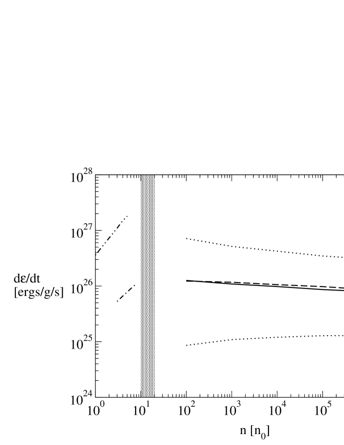
FIG. 4.: Emissivity from quark matter for high densities of $100-10^{7}n_{0}$. The solid [dashed] line shows the result using the formula for the QCD coupling constant derived from the ${\beta}$-function to ${\cal O}({\alpha}_{s}^{4})$ [${\cal O}({\alpha}_{s}^{2})$]. The cutoff mass $m_{D}$ is calculated using Eq. (41). The upper and lower dotted lines correspond to a cutoff mass of $m_{D}/3$ and $3m_{D}$, respectively. The results for nuclear matter at lower densities from Ref. [16] are also included, using the approximations for degenerate (dot-dashed line) and non-degenerate matter (dot-dot-dashed line). All calculations are for the case of $d=2$ extra dimensions and a temperature of $T=50$ MeV; the size of the extra dimensions is taken to be 1 mm. The gray area denotes the region of realistic density of $n_{q}\approx 10-20n_{0}$.

we show the graviton emission rate from quark matter for a density range of $100-10^{7}n_{0}$ for the case of $d=2$ extra dimensions and a temperature of $T=50$ MeV, assuming that the size of the extra dimensions is $R=1$ mm. The solid line shows the result using the cutoff mass $m_{D}$ calculated from Eq. (41) valid for small ${\alpha}_{s}$ and using the formula Eq. (32) for the QCD coupling constant derived from the ${\beta}$-function to ${\cal O}({\alpha}_{s}^{4})$. To estimate the error introduced by calculating only first order diagrams we give also the result for the emissivity using the (larger) ${\alpha}_{s}$ [see Eq. (31)] calculated from the ${\beta}$-function to ${\cal O}({\alpha}_{s}^{2})$ (dashed line). This results in an increase in the cross section which gets partially compensated by a larger cutoff mass. Therefore the emissivities for both values of ${\alpha}_{s}$ are very similar.

To account for uncertainties in the cutoff mass (higher order corrections, unaccounted many-body effects) $m_{D}$ we also show the emissivity using $m_{D}/3$ (upper dotted line) and $3m_{D}$ (lower dotted line). With $m_{D}$ spanning about one order of magnitude in the cutoff mass the emissivity varies by about 1-2 orders of magnitude. We also present the emission rates from nucleon-nucleon scattering [16] for lower densities.

Note that it is not sensible to compare the emission rates for quark matter and nuclear matter for an equal density, since for densities much higher than $5n_{0}$ nucleons are certainly no longer the appropriate degrees of freedom. Similarly, for densities smaller than about $100n_{0}$ the QCD coupling constant becomes too large so that perturbative QCD calculations will no longer be applicable. It is therefore necessary to extrapolate from the two regions where reliable calculations are possible to the interesting transition region with $n_{q}=10-20n_{0}$ (gray area in Fig. 4).

Determining the emissivity for the physical density region from Fig. 4 for $d=2$ and carrying out a similar analysis for $d=3$, we can now use the Raffelt criterion, limiting the energy lost into any non-standard physics channel to $10^{19}$ ergs/g/s, to calculate bounds on the size of new extra dimensions. The radius $R$ enters the calculation through the prefactors in Eqs. (53) and (58). Our bounds are calculated to be

$$R < 2.9\times 10^{-4}\text{mm}\quad\text{for }n=2\quad\text{and}$$ (63)

$$R < 3.9\times 10^{-7}\text{mm}\quad\text{for }n=3$$ (64)

which are quite similar to the ones determined for nuclear matter [16].

It should be kept in mind that these bounds become somewhat weaker [stronger] as $m_{D}$ is taken to larger [smaller] values thereby decreasing [increasing] the emissivity. Our conservative estimates are therefore weaker than those found from previous nuclear matter calculations.

VI Conclusion

Supernovas like SN1987a provide one of the most stringent constraints on the size of gravity-only extra dimensions. Bounds on these sizes have been calculated before [14, 15, 16, 17] assuming a density of $\approx 1-3n_{0}$ and a typical temperature of $T\approx 50$ MeV where matter is nucleonic. The relevant degrees of freedom for this regime are protons and neutrons.

In view of the uncertainties with which the parameters governing the condition of matter at the star’s inner core, such as density and temperature, are given, and in view of the fact that, as can be found from various nuclear matter equations of state, matter in the star’s core lies very close to a phase transition to either a deconfined QCD plasma or, for lower temperatures, a color superconducting phase, it is worthwhile and important to investigate how emission rates and bounds on the radius of the extra dimensions change in these regimes.

In this paper we have calculated emissivities and bounds on the size of gravity-only extra dimensions from a deconfined quark-gluon plasma in the core of a star seconds after the supernova core bounce. We have not considered the case where the temperature falls below the critical temperature $T_{c}$ defining the transition of quark matter to a color superconducting state.

By extrapolating the emissivity from a quark-gluon plasma at very high density ($n_{q}=100n_{0}-10^{7}n_{0}$) down to the physically interesting region of $n_{q}\approx 10-20n_{0}$ we find that the KK-graviton emissivity is comparable to those found from nuclear matter calculations. We have examined the error introduced into our calculation due to the fact that we are working only to first order in the QCD coupling constant. We estimate this error to be at the most 100%. To consider the rather uncertain value of the cutoff mass we have calculated the emissivity using a cutoff mass which varies about one order of magnitude about the central value from the lowest order perturbative calculation [Eq. (41)]. We find that this causes an uncertainty in the emissivity of about two orders of magnitude.

We have not examined any other many-body effects which could modify the vacuum rates for KK-graviton emission, such as the Landau-Pomeranchuk-Migdal effect, which would decrease the emissivity because of multiple quark scattering before the graviton gets emitted.

Note that the source of uncertainties is not the soft radiation theorem, which is well suited for the degenerate case, but rather our lack of knowledge about the nuclear physics nature of QCD. This deficit of understanding to only impacts our calculation of the quark-quark scattering cross section and the treatment of the QCD plasma, but also forces us to access the interesting transition region only with the aid of extrapolation.

Despite the significant uncertainties in our calculation for quark matter, we believe to have ruled out the possibility of a significantly larger emissivity compared to the nuclear matter case. It is up to further investigation to provide better information on the conditions which govern the state of the matter at the star’s core during and shortly after a supernova event. It is unlikely that the whole core will consist of dense quark matter, more likely is a scenario where at the core’s center matter is deconfined and undergoes a phase transition to nuclear matter as one goes towards the surface. Furthermore, a better understanding of QCD in the non-perturbative regime and at finite density would enable a reduction of the uncertainties.

A Results for the Angular Integration

The functions $g_{X}(x,y,{\theta_{\text{cm}}})$ defined in Eq. (23) are calculated for the three cases of 4D-graviton ($g$), KK-graviton ($h$), and KK-dilaton ($\phi$) to be

$$g_{g} = \frac{1}{4}\Biggl{\{}-1+y^{2}+\frac{(1+6y^{2}+y^{4})\log\frac{y+1}{y-1}}{2y}-\frac{2y^{2}+y^{4}+4y^{2}\cos{\theta_{\text{cm}}}+\cos 2{\theta_{\text{cm}}}}{{\cal W}(x,y,\cos{\theta_{\text{cm}}})}$$ (A3)

$$\quad\times\log\frac{-(y^{2}-1)^{2}+2(y^{2}+\cos{\theta_{\text{cm}}})^{2}+2(y^{2}+\cos{\theta_{\text{cm}}}){\cal W}(x,y,\cos{\theta_{\text{cm}}})}{(y^{2}-1)^{2}}\Biggr{\}}$$

$$+\frac{1}{4}\Biggl{\{}\cos{{\theta_{\text{cm}}}}\rightarrow-\cos{{\theta_{\text{cm}}}}\Biggr{\}},$$

$$g_{h} = \frac{1}{6}\sqrt{1-x^{2}}\Biggl{\{}\frac{4(y^{2}-1)^{2}}{x^{2}+y^{2}-1}+\frac{2(y^{4}+4y^{2}+1)\log\frac{y+\sqrt{1-x^{2}}}{y-\sqrt{1-x^{2}}}}{\sqrt{1-x^{2}}y}$$ (A7)

$$\quad+\frac{12y^{2}\cos{\theta_{\text{cm}}}+(2y^{2}+1)^{2}+3\cos 2{\theta_{\text{cm}}}}{(x^{2}-1){\cal W}(x,y,\cos{\theta_{\text{cm}}})}$$

$$\qquad\times\log\frac{(x^{2}-1)\left[-\frac{(x^{2}+y^{2}-1)^{2}}{(x^{2}-1)}+2\left(\frac{y^{2}}{1-x^{2}}+\cos{\theta_{\text{cm}}}\right)^{2}+2\left(\frac{y^{2}}{1-x^{2}}+\cos{\theta_{\text{cm}}}\right){\cal W}(x,y,\cos{\theta_{\text{cm}}})\right]}{(x^{2}+y^{2}-1)^{2}}\Biggr{\}}$$

$$+\frac{1}{6}\sqrt{1-x^{2}}\Biggl{\{}\cos{{\theta_{\text{cm}}}}\rightarrow-\cos{{\theta_{\text{cm}}}}\Biggr{\}},$$

and

$$g_{\phi} = \frac{d-1}{3(d+2)}\sqrt{1-x^{2}}(y^{2}-1)\Biggl{\{}\frac{y^{2}-1}{x^{2}+y^{2}-1}+\frac{(y^{2}-1)\log\frac{y+\sqrt{1-x^{2}}}{y-\sqrt{1-x^{2}}}}{2\sqrt{1-x^{2}}y}+\frac{y^{2}-1}{(x^{2}-1){\cal W}(x,y,\cos{\theta_{\text{cm}}})}$$ (A10)

$$\quad\times\log\frac{(x^{2}-1)^{2}\left[-\frac{(x^{2}+y^{2}-1)^{2}}{(x^{2}-1)^{2}}+2\left(\frac{y^{2}}{1-x^{2}}+\cos{\theta_{\text{cm}}}\right)^{2}+2\left(\frac{y^{2}}{1-x^{2}}+\cos{\theta_{\text{cm}}}\right){\cal W}(x,y,\cos{\theta_{\text{cm}}})\right]}{(x^{2}+y^{2}-1)^{2}}\Biggr{\}}$$

$$+\frac{d-1}{3(d+2)}\sqrt{1-x^{2}}(y^{2}-1)\Biggl{\{}\cos{{\theta_{\text{cm}}}}\rightarrow-\cos{{\theta_{\text{cm}}}}\Biggr{\}}.$$

The function ${\cal W}(x,y,h)$, introduced for convenience, is defined as

$${\cal W}(x,y,h)=\sqrt{\frac{(h+1)[-x^{2}-2y^{2}+(x^{2}-1)h+1]}{x^{2}-1}}.$$ (A11)

REFERENCES

• [1] D. E. Groom et al., Eur. Phys. J. C15, 1 (2000).
• [2] N. Arkani-Hamed, S. Dimopoulos, and G. Dvali, Phys. Lett. B429, 263 (1998), hep-ph/9803315.
• [3] N. Arkani-Hamed, S. Dimopoulos, and G. Dvali, Phys. Rev. D59, 086004 (1999), hep-ph/9807344.
• [4] I. Antoniadis, N. Arkani-Hamed, S. Dimopoulos, and G. Dvali, Phys. Lett. B436, 257 (1998), hep-ph/9804398.
• [5] L. Randall and R. Sundrum, Phys. Rev. Lett. 83, 3370 (1999), hep-ph/9905221.
• [6] C. D. Hoyle et al., (2000), hep-ph/0011014.
• [7] T. Han, J. D. Lykken, and R.-J. Zhang, Phys. Rev. D59, 105006 (1999), hep-ph/9811350.
• [8] G. F. Giudice, R. Rattazzi, and J. D. Wells, Nucl. Phys. B544, 3 (1999), hep-ph/9811291.
• [9] J. L. Hewett, Phys. Rev. Lett. 82, 4765 (1999), hep-ph/9811356.
• [10] L. Vacavant and I. Hinchliffe, (2000), hep-ex/0005033.
• [11] I. Antoniadis and K. Benakli, (2000), hep-ph/0004240.
• [12] M. Fairbairn, (2001), hep-ph/0101131.
• [13] G. G. Raffelt, Stars as Laboratories for Fundamental Physics (The University of Chicago Press, 1996).
• [14] V. Barger, T. Han, C. Kao, and R. J. Zhang, Phys. Lett. B461, 34 (1999), hep-ph/9905474.
• [15] S. Cullen and M. Perelstein, Phys. Rev. Lett. 83, 268 (1999), hep-ph/9903422.
• [16] C. Hanhart, D. R. Phillips, S. Reddy, and M. J. Savage, (2000), nucl-th/0007016.
• [17] C. Hanhart, J. A. Pons, D. R. Phillips, and S. Reddy, (2001), astro-ph/0102063.
• [18] K. Rajagopal and F. Wilczek, (2000), hep-ph/0011333.
• [19] P. J. Fox, (2000), hep-ph/0012165.
• [20] F. E. Low, Phys. Rev. 110, 974 (1958).
• [21] A. L. Adler and Y. Dothan, Phys. Rev. 151, 1267 (1966).
• [22] C. Hanhart, D. R. Phillips, and S. Reddy, (2000), astro-ph/0003445.
• [23] S. Weinberg, Gravitation and Cosmology: Principles and Applications of the General Theory of Relativity (John Wiley and Sons Inc, 1972).
• [24] N. Iwamoto, Ann. Phys. 141, 1 (1982).
• [25] B. L. Combridge, J. Kripfganz, and J. Ranft, Phys. Lett. B70, 234 (1977).
• [26] H. Heiselberg and C. J. Pethick, Phys. Rev. D48, 2916 (1993).
• [27] M. L. Bellac, Thermal Field Theory (Cambridge University Press, 1996).
• [28] P. Morel and P. Nozières, Phys. Rev. 126, 1909 (1962).
• [29] G. Baym and C. Pethick, in The Physics of Liquid and Solid Helium, edited by K. H. Bennemann and J. B. Ketterson (Wiley, 1978), Pt. II.