Continuum QRPA in the coordinate space representation
Abstract
We formulate a quasi-particle random phase approximation (QRPA) in the coordinate space representation. This model is a natural extension of the RPA model of Shlomo and Bertsch to open-shell nuclei in order to take into account pairing correlations together with the coupling to the continuum. We apply it to the 120Sn nucleus and show that low-lying excitation modes are significantly influenced by the pairing effects although the effects are marginal in the giant resonance region. The dependence of the pairing effect on the parity of low-lying collective mode is also discussed.
pacs:
PACS numbers: 21.60.Jz, 21.60.-n, 21.10.Re,23.20.-gI Introduction
The random phase approximation (RPA) has provided a convenient and useful method to describe excited states of many-fermion systems. There are a number of ways to formulate the RPA [1, 2, 3, 4, 5, 6, 7, 8, 9]. In practical point of view, we particularly mention here a configuration space formalism and a response function formalism. The configuration space formalism diagonalizes a non-hermitian matrix denoted often by and matrices which are constructed in the model space of 1 particle-1 hole (1p-1h) states. In contrast, the response function formalism is based on the linear response theory and solves a Bethe-Salpeter equation for the response function, often in the coordinate space [5, 7, 8]. The response function formalism can be formulated in various representations of basis states, and the connection between these two methods can be made by expressing response functions in the configuration space [1].
The response function formalism of RPA becomes particularly simple when the interaction is a zero-range contact force. In that case, the excitations to particle continuum states can be treated exactly by solving the single-particle Green function in the coordinate space. This method was first developed by Shlomo and Bertsch [5] and subsequently applied to self-consistent calculations of nuclear giant resonances with Skyrme interaction by Liu and Van Giai [10]. Recently it has been extensively used by Hamamoto, Sagawa, and Zhang to discuss giant resonances of neutron-rich nuclei, where the continuum effects play an essential role due to a much lower threshold energy compared with -stable nuclei [11, 12]. An extension to the three dimensional space has also been carried out recently by Nakatsukasa and Yabana for the study of atomic clusters [13]. The coupling between particle-particle continuum was also studied in 11Li by Bertsch and Esbensen[14, 15].
Although it has been well known that the pairing correlation plays an important role in the ground state of open-shell nuclei, it has been neglected in applying the response function formalism to describe excited states of atomic nuclei until very recently [16]. So far a simple filling approximation has been employed in open-shell nuclei in order to simulate the pairing correlations. However, it is important to take into account the pairing effects consistently for the study of excited states of open-shell nuclei, and thus the quasi-particle RPA (QRPA) should be used instead of the RPA [17].
The aim of this paper is to generalize the formalism of Shlomo and Bertsch to the QRPA and discuss the effects of pairing correlations on excited states of open-shell nuclei. In this paper, we study only cases where the BCS approximation works well and thus all states in the pairing active space are bound, leaving out as a future work a self-consistent treatment of the pairing effects in the continuum using the Hartree-Fock-Bogoliubov + RPA theory [18, 19, 20]. Our method is closely related to that in Ref. [16], although details are somewhat different. The paper is organized as follows. In Sec. II, we briefly review the formalism of Shlomo and Bertsch and extend it to the QRPA. In Sec. III, we apply the formalism to the isoscalar (IS) monopole, quadrupole, and octupole modes as well as the isovector (IV) dipole mode of excitation of the 120Sn nucleus and discuss the effects of pairing correlations on the excited states. A summary is given in Sec. IV.
II Linear Response Theory for Open-shell Nuclei
We begin with the configuration space formalism of the RPA theory and then make a connection to the response function method. The RPA equation can be given in a compact form
| (1) |
where and are the forward and the backward amplitudes, respectively. For a residual interaction of delta-type contact force, , the matrix elements of and for the -multipole mode read
| (2) |
where () denotes a particle (hole) state and is the reduced matrix element. The radial integral is given by
| (3) |
where is a single-particle radial wave function. We have absorbed the overall factor in front of the matrix by redefining the sign of the backward amplitudes.
The integral (3) can be computed by discretizing it as
| (4) |
where is the spacing of the radial coordinate. Since the interaction is then given as a sum of separable form, the RPA frequencies can be obtained by solving the generalized RPA dispersion relation [9], where the matrices and are given by
| (5) | |||||
| (6) |
respectively, in the coordinate space representation. Here, is a infinitesimal real number, and is given by
| (7) |
Note that is nothing but the unperturbed response function in the linear response theory. Here we introduce the RPA response function which obeys a Bethe-Salpeter equation
| (8) |
This equation can be solved in the coordinate space by matrix inversion as [7]
| (9) |
The response of the system to an external field is then given by [7]
| (10) |
The exact treatment of the continuum effects can be achieved by eliminating the sum of the particle states in the free response function (5) using the complete set of the wave function [5]. This leads to
| (12) | |||||
where is the single-particle Hamiltonian, and the single-particle Green function is given by
| (13) |
Here, and are the regular and irregular solutions of the Hamiltonian at energy , and is the Wronskian given by .
In the application of the formalism to nuclear systems, we use the proton-neutron formalism which can properly take into account the couplings between the IS and IV modes of excitation [11]. The Bethe-Salpeter equation given by Eq. (8) is then generalized to be
| (14) |
For simplicity of the notation, we do not present below the formalism in the two-component form, although we indeed use it in the actual calculations given in the next section.
In the presence of paring correlations, the elementary excitation is a two quasi-particle excitation, rather than a particle-hole excitation. A generalization of the RPA to the QRPA is given in Ref. [3] together with relevant and matrices in the QRPA equation. A free response function in the QRPA in the configuration space representation can be constructed in a similar way to the RPA,
| (15) |
with
| (16) |
where is the BCS occupation probability and . is the quasi-particle energy given by , where and are the chemical potential and the pairing gap, respectively. In the BCS approximation, is an eigenfunction of the single-particle Hamiltonian with an eigen-energy . Since the quasi-particle energy is not an eigenvalue of in general, it is not straightforward to introduce the single-particle Green function (13) in the QRPA free response function. However, when the pairing gap is zero for states outside the pairing active space, the quasiparticle energy becomes an eigenvalue of the single-particle Hamiltonian, i.e. , and =1. We therefore consider separately excitations among states within the pairing active space and those from the inside to the outside of the active space. To the latter model space, we apply the same procedure as the RPA response function. The free response function in the BCS approximation (15) thus becomes
| (17) | |||
| (18) | |||
| (19) | |||
| (20) |
where the summations of and are restricted to the states within the pairing active space. The last term in Eq. (20) is a correction for a double-counting of excitations within the pairing active space, which stems from the substitution of the completeness relation in Eq. (15). Note that, without the pairing correlations, and for , and the BCS free response function (20) is identical to the corresponding response function (12) in the RPA. With this unperturbed response function (20), the QRPA response function is obtained again by solving the Bethe-Salpeter equation (8) as in the RPA theory.
III Continuum QRPA Excitations in 120Sn
We now apply the continuum QRPA formalism to 120Sn and make a comparison between the QRPA and the RPA. We choose this system because it is a typical open-shell nucleus and also because it is a sub-shell closure nucleus where the RPA can be applied unambiguously without using the filling approximation for valence nucleons. The single-particle wave functions and the single-particle energies are obtained by solving the Shrödinger equation with a Woods-Saxon mean-field potential. As a residual interaction , we use the and parts of the Skyrme residual interaction, which is obtained from the second derivative of the Skyrme energy functional with respect to the proton and the neutron densities. The ground state density to be used in the density-dependent part of the residual interaction is generated from the single-particle wave functions . We use the same parameters as those in Ref. [5] for the mean-field potentials and the residual interaction, i.e., 1100 MeV fm3, 16000 MeV fm6, =0.5, =1, and =1 in the standard notation of the Skyrme functional [21]. Since this model is not self-consistent, we renormalize for the QRPA and the RPA calculations, respectively, so that the spurious IS dipole mode appears at zero excitation energy. The resultant renormalization factors are = 0.638 and 0.660 for RPA and QRPA, respectively. For the pairing of neutrons, we use a schematic state-independent constant pairing gap MeV, which is estimated from the experimental binding energies of neighboring nuclei. The pairing active space which we adopt includes the levels up to the major shell as well as the 1g7/2, 2d5/2, 2d3/2, 3s1/2, and 1h11/2 levels. The single-particle energy for the valence levels are shown in Table 1, together with the BCS occupation probabilities. The proton pairing gap is set to be zero due to the magic number .
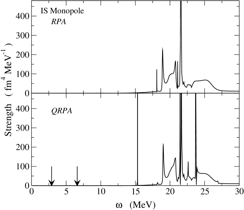
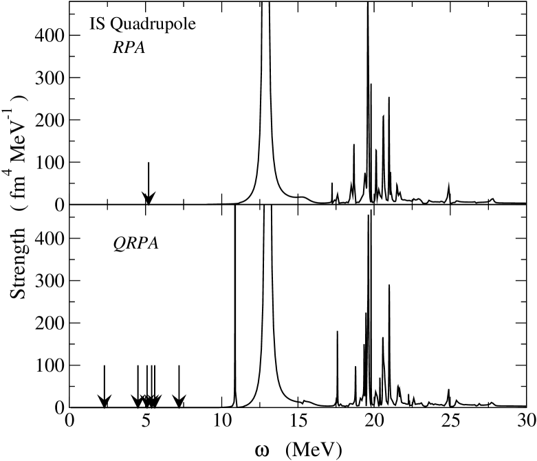
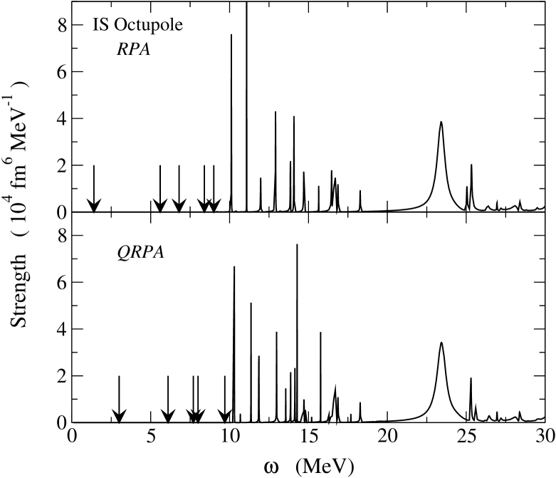
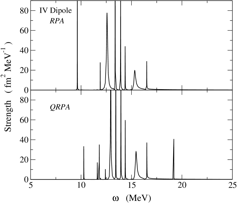
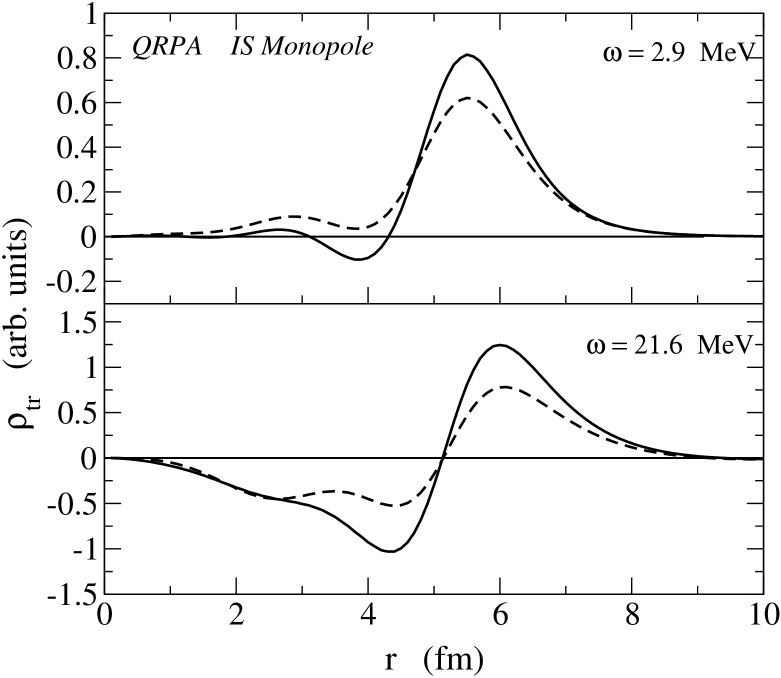
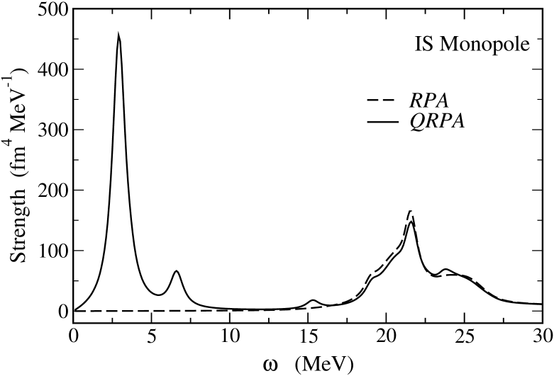
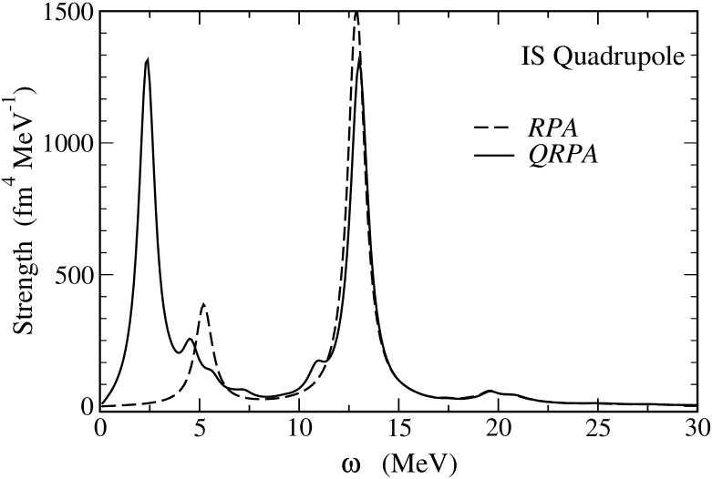
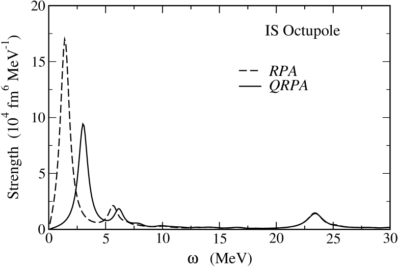
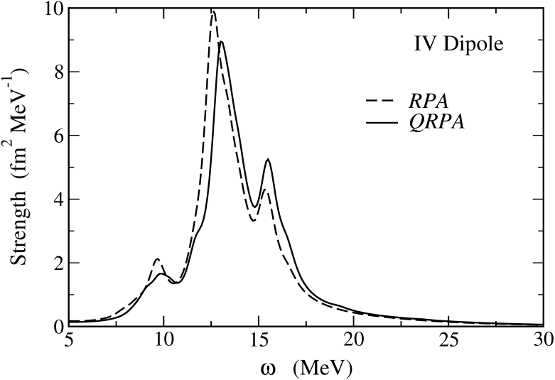
Figs. 1–4 show the strength function for the isoscalar (IS) monopole, IS quadrupole, IS octupole, and the isovector (IV) dipole modes of excitations, respectively. The external field for each modes is given by , , , and , respectively. The lower panels show results of the QRPA calculations, while the upper panels show results of the RPA calculations without the pairing correlations as a comparison. For the latter, the levels up to 3s1/2 state are occupied with the occupation probability of 1, while those above 1h11/2 state are unoccupied with (see Table 1). Arrows indicate the positions of (Q)RPA states below the threshold, where the strength function has no width.
For the monopole excitation shown in Fig.1, the RPA does not show any low-lying mode, although the experimental second lowest state in the 120Sn nucleus is observed at the excitation energy 1.874 MeV, which is attributed to a paring vibration mode. The second lowest state in the QRPA is found at rather low energy 2.9 MeV, and may couple to the pairing vibrational mode. The IS giant monopole states are seen in the energy region 1728 MeV in both the QRPA and RPA calculations. The transition densities for the IS monopole mode at two different energies, i.e., = 2.9 MeV and 21.6 MeV, are shown in Fig. 5. We find that the former shows a characteristic behaviour of the pairing vibration mode while the latter shows the compressional character. For the quadrupole mode shown in Fig. 2, the lowest RPA state is at 5.2 MeV, in comparison with the experimental value of 1.17 MeV. The transition strength is B(E2:0)= 0.031 in the RPA calculation, while the experimental value is 0.2 . If one takes the pairing correlations into account, the low-lying 2+ RPA states goes substantially down and the lowest QRPA state appears at 2.3 MeV having the transition strength B(E2:0)= 0.107 , which is much closer to the experimental value. In both cases, the main peak of the IS giant quadrupole resonance (GQR) appears at around 13 MeV exhausting most of the sum rule strength. The experimental GQR is also observed at the excitation energy around 13MeV[22]. As for the octupole mode of excitations in Fig. 3, the experimental value of the lowest state is at 2.4 MeV, while the RPA and the QRPA lead to 1.4 MeV and 3.0 MeV, respectively. The experimental value for the corresponding transition rate is B(E3:0)= 0.09 , while it is 0.159 and 0.0771 in the RPA and the QRPA, respectively. The RPA without pairing correlations underestimates the lowest state energy and the QRPA is more satisfactory compared with the experimental value. We summarize in Table 2 the results of the RPA and the QRPA calculations together with the experimental data for the lowest 2+ and 3- states. Giant octupole resonances (GOR) are observed in Fig. 3 at the excitation energy 23 MeV in both cases. Results for the IV giant dipole resonance (GDR) are shown for RPA and QRPA in Fig. 4. As is the same as in Figs. 1–3, the structure of GDR is not much disturbed by the effect of the pairing.
Notice that the effect of the pairing on the low-lying quadrupole mode is opposite to that on the octupole mode. For the former, the energy of the lowest 2+ state becomes smaller due to the pairing, with enhancement of the B(E2) value. On the other hand, the QRPA raises the energy of the lowest 3- state and the B(E3) value is hindered. In both cases, the QRPA gives better agreement with the experimental values compared with the RPA. These features can be understood as follows. For excitations with even parity, such as the quadrupole excitations, transitions between the same levels are allowed in the presence of the pairing correlations. This enhances the collectivity of low-lying states, resulting in a smaller excitation energy and a larger transition strength. On the contrary, such excitations are not allowed for odd parity excitations, e.g., the octupole mode. In that case, the dominant excitation is from one major shell to another regardless of the pairing correlation. Since the particle-hole excitations are weakened by the factor in the presence of the pairing, the QRPA lowers the collectivity of low-lying collective excitations with odd parity.
In contrast to the low-lying modes of excitations, in general, high-lying modes are much less sensitive to the paring correlations. This is the case for all the modes of excitations shown in Figs. 1–4. This fact can be seen more transparently if one smears the strength functions with a finite width. We show in Figs. 6–9 the RPA and QRPA results with a finite value of =0.5MeV in Eq. (20). As one clearly sees, the two results resemble each other in the giant resonance region at energies above the threshold near 10 MeV. These results are natural consequences of the pairing correlations since the configurations outside the pairing active space are the main p-h configurations for the giant resonances and thus the pairing effects should play a minor role.
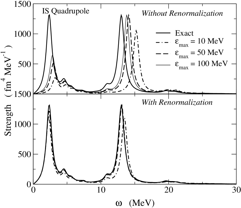
A conventional approximation to treat the continuum effect is to put a nucleus in a box and discretize the continuum states by imposing a boundary condition at the edge of the box. A model space of these states is usually truncated at the maximum single-particle energy . Since our continuum QRPA method can treat the coupling to the continuum exactly, it is interesting to compare our method with the box discretization approximation. Fig. 10 shows a convergence property of the box discretization method for the IS quadrupole response. We take the box size of =10 fm, and smear the strength function with =0.5 MeV for the representation purpose. We have checked that the results do not change significantly even if we use a larger value of . The solid line is the result of the continuum QRPA method with the exact treatment of the continuum effect, which is the same as in Fig. 6. The dot-dashed, dashed, and thin solid lines are results of the box discretization method with truncation energy at = 10, 50, and 100 MeV, respectively. In the upper panel, we use the same residual interaction for all the calculations. As one can see, the convergence with respect to the maximum energy of continuum states is extremely slow: even with = 100 MeV the peak positions are not reproduced. The peak height for the lowest energy peak is not reproduced, either. We note that the truncation of the model space shfts the position of the spurious IS dipole state. It appears at 6.0, 4.4, and 3.7 MeV for = 10, 50, and 100 MeV, respectively. In the lower panel, the renormalized residual interaction is used for each value of so that the IS dipole mode appears at zero energy. The renormalization factors are = 0.968, 0.776, and 0.732 for = 10, 50, and 100 MeV, respectively. This procedure drastically improves the convergence. In the case of the truncation energy = 50 MeV (dashed line), the exact solution is almost reproduced. The result converges at this energy and the shape of the strength function is not altered even when the states up to = 100 MeV are included. This study clearly indicates the importance of the self-consistency between the space truncation and the renormalization of the residual interaction. If this self-consistency is imposed, the box discretization method works well. It should be emphasized, however, that the escape width of resonances can be obtained only when the single-particle continuum states are treated exactly as we do in this article.
IV Summary and Discussions
We proposed a QRPA model in the coordinate space to take into account the continuum effects. It is a generalization of the formalism of Shlomo and Bertsch for the continuum RPA to the QRPA. We treated separately the p-h excitations within the pairing active space and those between the active space and the non-active space. For the former, we explicitly used the two quasiparticle configurations in the response function in the coordinate space, while for the latter we use the single-particle Green function in the coordinate space representation taking into account the coupling to the particle continuum properly. We applied the formalism to 120Sn and showed that the pairing correlations enhance the collectivity of the positive parity low-lying states, while that of the negative parity low-lying states are hindered. We found that the QRPA is more satisfactory in reproducing the experimental data of the energy of low-lying modes of excitation, while the giant resonances are not much affected by the pairing correlations. We would like to point out that these results however do not justify the RPA model without the pairing correlations for the study of giant resonances in open-shell nuclei, especially near the drip-lines. Since the single-particle energies and wave functions could be different in principle due to the density dependence of the mean-field, the response properties even in the giant resonance region might be affected by the pairing correlations. We therefore advocate to use the QRPA all through the excitation region in open-shell nuclei.
There are many possible applications of the continuum QRPA method presented in this paper. One of them is a neutrino-nucleus scattering, e.g. 12C()12C∗ [23] and 12C()12N [24], where the RPA and the QRPA have been one of the standard methods for theoretical investigations. Another application will be the excitations of drip-line nuclei. Because of a low energy threshold, the responses would be very sensitive to the pairing correlations. In these cases, the pairing active space includes particle continuum states and the BCS approximation should be carefully examined. Also, the residual interaction in the particle-particle channel, which we neglected in this paper, might have to be taken into account. A more sophisticated treatment of the pairing interaction is provided by the Hartree-Fock-Bogoliubov (HFB) theory, which consistently describes couplings between the particle-hole and the particle-particle channels. It would be an interesting future work to develop a continuum QRPA theory based on the HFB approximation.
Acknowledgment
We are grateful to the Institute for Nuclear Theory at the University of Washington, where this work was initiated during the INT program INT-00-3 on “Nuclear structure for the 21st century”. We thank its hospitality and a partial financial support for this work. We thank also K. Matsuyanagi and Nguyen Van Giai for useful and stimulating discussions and Baha Balantekin for discussions on the RPA approach to neutrino-nucleus reactions. This work is supported in part by the Ministry of Education, Science, Sports and Culture in Japan by Grant-In-Aid for Scientific Research under the program number (C(2)) 12640284.
REFERENCES
- [1] G.F. Bertsch and R.A. Broglia, Oscillations in Finite Quantum Systems (Cambridge University Press, Cambridge, 1994).
- [2] A.L. Fetter and J.D. Walecka, Quantum Theory of Many-Particle Systems (McGraw-Hill, New York, 1971).
- [3] D.J. Rowe, Nuclear Collective Motion (Methuen, London, 1968).
- [4] P. Ring and P. Schuck, The Nuclear Many Body Problem (Springer-Verlag, New York, 1980).
- [5] S. Shlomo and G. Bertsch, Nucl. Phys. A243, 507 (1975).
- [6] P.-G. Reinhard and Y.K. Gambhir, Annalen der Physik 1, 598 (1992).
- [7] G.F. Bertsch and S.F. Tsai, Phys. Rep. 18, 126 (1975).
- [8] S.F. Tsai, Phys.Rev. C17, 1862 (1978).
- [9] Nguyen Van Giai, Ch. Stoyanov, and V.V. Voronov, Phys. Rev. C57, 1204 (1998).
- [10] K.F. Liu and Nguyen Van Giai, Phys. Lett. 65B, 23 (1976).
- [11] I. Hamamoto, H. Sagawa, and X.Z. Zhang, Phys. Rev. C55, 2361 (1997); Phys. Rev. C57, R1064 (1998).
- [12] I. Hamamoto and H. Sagawa, Phys. Rev. C60, 064314 (1999); Phys. Rev. C62, 024319 (2000).
- [13] T. Nakatsukasa and K. Yabana, e-print: physics/0010025.
- [14] G.F. Bertsch and H. Esbensen, Ann. of Phys. (N.Y.) 209, 327 (1991).
- [15] H. Esbensen and G.F. Bertsch, Nucl. Phys. A542, 310 (1992).
- [16] S. Kamerdzhiev, R.J. Liotta, E. Litvinova, and V. Tselyaev, Phys. Rev. C58, 172 (1998).
- [17] E. Khan and Nguyen Van Giai, Phys. Lett. B472, 253 (2000).
- [18] J. Dobaczewski, W. Nazarewicz, T.R. Werner, J.F. Berger, C.R. Chinn, and J. Dechargé, Phys. Rev. C53, 2809 (1996).
- [19] S.A. Fayans, S.V. Tolokonnikov, E.L. Trykov, and D. Zawischa, Nucl. Phys. A676, 49 (2000).
- [20] Nguyen Van Giai, M. Grasso, R.J. Liotta, and N. Sandulescu, e-print: nucl-th/0010022.
- [21] D. Vautherin and D.M. Brink, Phys. Rev. C5, 626 (1972).
- [22] A. van der Woude, Proc. of Giant Multipole Resonance Topical Conference (ed. F. E. Bertrand, Oak Rigde, 1979) p. 65
- [23] N. Jachowicz, S. Rombouts, K. Heyde, and J. Ryckebusch, Phys. Rev. C59, 3246 (1999).
- [24] C. Volpe, N. Auerbach, G. Coló, T. Suzuki, and N. Van Giai, Phys. Rev. C62, 015501 (2000).
| level | energy (MeV) | occupation probability |
|---|---|---|
| 1g7/2 | 11.184 | 0.954 |
| 2d5/2 | 11.145 | 0.953 |
| 2d3/2 | 9.280 | 0.815 |
| 3s1/2 | 9.048 | 0.771 |
| 1h11/2 | 6.949 | 0.173 |
| E (MeV) | B(E2)(e2b2) | E (MeV) | B(E3)(e2b3) | |
|---|---|---|---|---|
| RPA | 5.2 | 0.031 | 1.4 | 0.159 |
| QRPA | 2.3 | 0.105 | 3.0 | 0.0771 |
| Expt | 1.17 | 0.2 | 2.4 | 0.09 |