comfeyn curly_len2mm dash_len1.5mm wiggly_len3mm

vardef ellipseraw (expr p, ang) = save radx; numeric radx; radx=6/10 length p; save rady; numeric rady; rady=3/10 length p; pair center; center:=point 1/2 length(p) of p; save t; transform t; t:=identity xscaled (2*radx*h) yscaled (2*rady*h) rotated (ang + angle direction length(p)/2 of p) shifted center; fullcircle transformed t enddef; style_def ellipse expr p= shadedraw ellipseraw (p,0); enddef;

NT@UW-00-022

TRI-PP-00-62

TUM-T39-00-18

21st December 2000

Nucleon Polarisabilities from
Compton Scattering on the Deuteron

Harald W. Grießhammer ${}^{a,\,}$ and Gautam Rupak ${}^{b,\,c,\,}$

^aInstitut für Theoretische Physik, Physik-Department,
Technische Universität München, D-85747 Garching, Germany
^bNuclear Theory Group, Department of Physics, University of Washington,
Box 351560, Seattle, WA 98195-1560, USA
^cTRIUMF, Vancouver, B.C., V6T 2A3, Canada

An analytic calculation of the differential cross section for elastic Compton scattering on the deuteron at photon energies $\omega$ in the range of $25-50\;\mathrm{MeV}$ is presented to next-to-next-to-leading order, i.e. to an accuracy of $\sim 3\%$. The calculation is model-independent and performed in the low energy nuclear Effective Field Theory without dynamical pions. The iso-scalar, scalar electric and magnetic nucleon polarisabilities $\alpha_{0}$ and $\beta_{0}$ enter as free parameters with a theoretical uncertainty of about $20\%$. Using data at $\omega_{\mathrm{Lab}}=49\;\mathrm{MeV}$ we find $\alpha_{0}=8.4\pm 3.0(\mathrm{exp})\pm 1.7(\mathrm{theor})$, $\beta_{0}=8.9\pm 3.9(\mathrm{exp})\pm 1.8(\mathrm{theor})$, each in units of $10^{-4}\;\mathrm{fm}^{3}$. With the experimental constraint for the iso-scalar Baldin sum rule, $\alpha_{0}=7.2\pm 2.1(\mathrm{exp})\pm 1.6(\mathrm{theor})$, $\beta_{0}=6.9\mp 2.1(\mathrm{exp})\mp 1.6(\mathrm{theor})$. A more accurate result can be achieved by: (i) better experimental data, and (ii) a higher order theoretical calculation including contributions from a couple of so far undetermined four-nucleon-two-photon operators.

Suggested PACS numbers: 13.60.Fz, 14.20.Dh, 21.30.Fe, 25.20.-x Suggested Keywords: Effective Field Theory, nucleon and neutron polarisability, deuteron Compton scattering

Albeit scalar electric and magnetic polarisabilities are fundamental properties of the neutron, there is a fair amount of uncertainty in their values for the lack of free neutron targets. Thus, one has to resort to indirect methods to extract neutron polarisabilities. For example, Rose et. al. depend on a particular treatment of the neutron as a quasi-free particle inside the deuteron and find for inelastic Compton scattering on the deuteron $\gamma d\rightarrow\gamma np$ that $\alpha^{(n)}=10.7^{+3.3}_{-10.7}$ [1]. Since the strong electromagnetic field of a heavy nucleus could enhance small effects from polarisability contributions, neutron scattering off a heavy nucleus is another method employed. However, analyses of low energy neutron-lead scattering experiments give conflicting values: $\alpha^{(n)}=12.3\pm 1.5\pm 2.0$, $\beta^{(n)}=3.1\mp 1.5\mp 2.0$ in Ref. [2], and more recently as part of an investigation of additional nuclei $\alpha^{(n)}=0\pm 5$ in Ref. [3]. In contradistinction, the scalar proton polarisabilities are well-measured from Compton scattering off the proton [4]: $\alpha^{(p)}=12.1\pm 0.8\pm 0.5$ and $\beta^{(p)}=2.1\mp 0.8\mp 0.5$, respectively.

On the theoretical side, a self-consistent and controlled description of the polarisabilities is only encountered with the dawn of Chiral Perturbation Theory ($\chi$PT) [5]. Unfortunately, estimates of corrections beyond leading order (LO) in $\chi$PT are difficult due to unknown parameters which already enter at next-to-leading order (NLO) [6, 7]. In this paper, we propose low energy Compton deuteron scattering as a probe for neutron polarisabilities. This is not a new idea and has fervently been advocated by Levchuk and L’vov, by Weyrauch, and by Arenhövel, Wilhelm and Wilbois, most recently in Refs. [8, 9, 10]; for its history see Ref. [11] and references therein. That the $\chi$PT values for the iso-scalar polarisabilities are consistent with Compton scattering data on the deuteron was demonstrated in two Effective Field Theory (EFT) NLO calculations in extensions of $\chi$PT to the few nucleon system, one using perturbative pions [12], one using non-perturbative pions [13].

The present calculation is unique in the sense that all the theoretical approximations are explicit and controlled, up to the order of the perturbative EFT calculation. The polarisabilities extracted from this calculation are independent of any modelling of the short-distance dynamics of nucleons inside a deuteron or any heavy nucleus. In particular, they are independent of assumptions about the pion-nucleon interaction, independent of the form of the inter-nucleon potential, manifestly independent of the photon coupling to nucleons and pions as extended objects and independent of the choice of regulator. The calculation is analytic and straightforward. To the accuracy claimed, the only experimental inputs are simple low energy observables: the binding energy and pole residue of the deuteron, the nucleon iso-vector magnetic moment and the nucleon-nucleon scattering length in the ${}^{1}\mathrm{S}_{0}$ channel. Our result will therefore – to the accuracy claimed – be reproduced by any “realistic” potential model, and can hence serve as cross check. However, at higher orders beyond those presented here, there are contributions from certain four-nucleon-two-photon operators representing short-distance physics that might not be reproduced accurately in a model calculation. In conclusion, the polarisabilities are obtained in a model independent way by a fit to data, and no explanation as to their origin is attempted.

The letter is organised as follows: We start by outlining the framework of the calculation and the power counting needed to determine the theoretical accuracy. Then, the amplitude and cross section is presented. Finally, various fits of the polarisabilities to data are discussed. A more detailed presentation will be given in an upcoming article [14].

Our analysis is in the context of the few-nucleon EFT in which nucleons and photons are the only dynamical degrees of freedom [15]. This formulation can be viewed as a systematisation of Effective Range Theory to include interactions with gauge fields, and relativistic and short-distance effects. Contributions from pions and other, heavier degrees of freedom are included at low energy through multiple-nucleon-photon contact interactions in perturbation. Since one cannot apply this EFT at energies where cuts in the amplitude are probed due to pion propagation, meson exchange etc., the natural breakdown scale $\Lambda$ is the pion mass $m_{\pi}\approx 140\;\mathrm{MeV}$. For details of the formalism, we refer to a recent review [16].

EFTs live from the fact that at low energies, a separation of scales exists: Like the binding momentum of the deuteron $\gamma=45.7066\;\mathrm{MeV}$, the photon momentum $\vec{k}$ and energy $\omega=|\vec{k}|$ are much smaller than $\Lambda$. There is another “high-energy” scale, namely the iso-spin averaged nucleon mass $M_{N}=938.92\;\mathrm{MeV}$. Thus, each physical low energy observable at a typical momentum scale $Q\sim\gamma$ is expanded systematically in powers of two small parameters: $\frac{Q}{\Lambda}$ and $\frac{Q}{M_{N}}$. For convenience, we formally identify $\Lambda/M_{N}\sim Q/\Lambda$, which is accidentally valid. Thus, relativistic corrections with a typical size $\gamma^{2}/M_{N}^{2}\sim(Q/M_{N})^{2}=(Q/\Lambda)^{2}\times(\Lambda/M_{N})^{2}$ contribute at $\mathcal{O}((Q/\Lambda)^{4})$, i.e. N⁴LO, see Refs. [15, 17, 18].

The centre-of-mass photon energy $\omega$ and the conversion of relativistic photon energies to non-relativistic nucleon energies introduce new scales: $\omega$ and $\sqrt{\omega M_{N}}$. Therefore, it is convenient to separate the calculation into two different energy régimes [12]. In régime I, $\omega\lesssim\gamma^{2}/M_{N}$, and $\sqrt{M_{N}\omega}\sim\gamma\sim Q$. We concentrate on régime II, i.e. higher photon energies $\omega\sim\gamma\sim Q$, in which factors of $\sqrt{\omega M_{N}}\sim\Lambda$ are summed to all orders. In addition, we make some integral approximations that allow us to effortlessly move from one régime to another with one simple expression [12]. Details of the power counting, calculation and validity of the approximations will be provided in a future publication [14].

In the Weyl gauge $A_{0}=0$, the amplitude for Compton scattering can be written as

$$\mathrm{i}\mathcal{A} = \mathrm{i}\;\frac{e^{2}}{2M_{N}}\left[S\;\vec{\varepsilon}_{d}\cdot\vec{\varepsilon}^{\prime\ast}_{d}+V_{i}\;\epsilon_{ijk}\;\varepsilon_{d,j}\varepsilon^{\prime\ast}_{d,k}+T_{ij}\;\left(\varepsilon_{d,i}\varepsilon^{\prime\ast}_{d,j}+\varepsilon_{d,j}\varepsilon^{\prime\ast}_{d,i}-\frac{2}{3}\delta_{ij}\ \vec{\varepsilon}_{d}\cdot\vec{\varepsilon}^{\prime\ast}_{d}\right)\right]\;\;,$$ (1)

representing the scalar $S$, vector $V$ and tensor $T$ coupling of a photon with incoming (outgoing) polarisation $\vec{\varepsilon}_{\gamma}$ ($\vec{\varepsilon}_{\gamma}^{\prime}$) with a deuteron of incoming (outgoing) polarisation $\vec{\varepsilon}_{d}$ ($\vec{\varepsilon}_{d}^{\prime}$). $\frac{e^{2}}{4\pi}=\alpha=1/137$. The power counting reveals that the vector and tensor amplitudes start contributing to the unpolarised cross section only at N⁴LO. Hence the most dominant term is the scalar one. The centre-of-mass scalar amplitude $S$ is conventionally written as

$$S = F(\omega,\theta)\;\vec{\varepsilon}_{\gamma}\cdot\vec{\varepsilon}^{\prime\ast}_{\gamma}+G(\omega,\theta)\;\left(\hat{\vec{k}}\times\vec{\varepsilon}_{\gamma}\right)\cdot\left(\hat{\vec{k}^{\prime}}\times\vec{\varepsilon}^{\prime\ast}_{\gamma}\right)\;\;,$$ (2)

where $F$ and $G$ represent the scalar electric and magnetic amplitudes, and $\theta$ is the angle between the directions of the incoming and outgoing photon momenta, $\hat{\vec{k}}$ and $\hat{\vec{k}^{\prime}}$. The familiar Thomson limit is reproduced by $F(\omega=0)=1$ and $G(\omega=0)=0$.

For $F$ and $G$, an expansion in powers of $Q/\Lambda$ exists, $F=F^{(0)}+F^{(1)}+\dots$ etc., where the superscript denotes the contribution of order $(Q/\Lambda)^{n}$. We keep all N²LO, i.e. $(Q/\Lambda)^{2}$, corrections compared to LO, $\mathcal{O}((Q/\Lambda)^{0})$. One such effect is the deuteron wave function renormalisation, introducing factors of $Z_{d}-1$. $Z_{d}=1.690(3)$ is the residue of the scattering amplitude at the deuteron pole and corresponds to the normalisation of the deuteron wave function at large wave length. $Z_{d}-1$ is treated as $\mathcal{O}(Q/\Lambda)$, see Ref. [19] for details. Higher order corrections such as relativistic effects and ${}^{3}\mathrm{S}_{1}$-${}^{3}\mathrm{D}_{1}$ mixing are irrelevant for the present N²LO calculation [15, 18]. Assuming that all contributions not taken into account are of natural size, we expect our result to be accurate to order $(Q/\Lambda)^{3}\lesssim 0.03$. This error estimate lies at the heart of a model-independent, controlled approximation provided by EFT.

Now for details of the calculation, performed in the centre-of-mass frame. The contribution from the seagull diagram in Fig. 1 (a) scales as $\mathcal{O}((Q/\Lambda)^{0})$, which constitutes a LO contribution in both energy régimes. We get

$$F^{(0)}_{a}=\frac{4\,{\sqrt{2}}\,\gamma\,}{\omega\,{\sqrt{1-\cos\theta}}}\;\arctan\left[\frac{\omega\,{\sqrt{1-\cos\theta}}}{2\,{\sqrt{2}}\,\gamma}\right]\;\;,$$

$$F^{(1)}_{a}=(Z_{d}-1)F^{(0)}_{a}\;\;,\;\;F^{(2)}_{a}=0\;\;,\;\;G_{a}=0\;\;.$$ (3)

(50,60) i o t1,t2 vanilla,width=thin,left=0.65i,o vanilla,width=thin,left=0.65,label=$\scriptstyle(a)$,label.side=left, label.dist=7o,i decor.shape=circle,decor.filled=shaded,foreground=red, decor.size=5i decor.shape=circle,decor.filled=shaded,foreground=red, decor.size=5o pa pavpath(__i,__o) photon,foreground=bluepoint 1/2 length(pa) of pa – vloc(__t1) photon,foreground=bluepoint 1/2 length(pa) of pa – vloc(__t2) (60,50) i1,i2,i3,i4,i5 o1,o2,o3,o4,o5 vanilla,width=thin,left=0.8v,i3 vanilla,width=thin,left=0.8i3,v vanilla,width=thin,left=0.8o3,v vanilla,width=thin,left=0.8v,o3 decor.shape=square,decor.size=5,foreground=green, label=${\scriptstyle(b)}$,label.angle=-90,label.dist=23v decor.shape=circle,decor.filled=shaded,foreground=red, decor.size=5i3 decor.shape=circle,decor.filled=shaded,foreground=red, decor.size=5o3 photon,foreground=bluei5,v,o5 (60,50) i1,i2,i3,i4,i5 o1,o2,o3,o4,o5 vanilla,width=thin,left=0.8v,i3 vanilla,width=thin,left=0.8i3,v vanilla,width=thin,left=0.8o3,v vanilla,width=thin,left=0.8v,o3 decor.shape=square,decor.size=5,foreground=green, label=${\scriptstyle(c)}$,label.angle=-90,label.dist=23v decor.shape=circle,decor.filled=shaded,foreground=red, decor.size=5i3 decor.shape=circle,decor.filled=shaded,foreground=red, decor.size=5o3 pa pb pavpath(__i3,__v) pbvpath(__v,__i3) photon,foreground=bluepoint 1/2 length(pa) of pa – vloc(__i5) photon,foreground=bluevloc(__o5) – point 1/2 length(pa) of pa (50,60) i o t1,t2 vanilla,width=thin,left=0.65i,o vanilla,width=thin,left=0.65,label=$\scriptstyle(d)$,label.side=left, label.dist=7o,i decor.shape=circle,decor.filled=shaded,foreground=red, decor.size=5i decor.shape=circle,decor.filled=shaded,foreground=red, decor.size=5o pa pavpath(__i,__o) upper upperpoint 1/2 length(pa) of pa photon,foreground=blueupper – vloc(__t1) photon,foreground=blueupper – vloc(__t2) decor.shape=circle,decor.filled=full,decor.size=10, label=$\scriptstyle\alpha_{0},,\beta_{0}$,label.angle=90,label.dist=9 upper (50,60) i o t1,t2 vanilla,width=thin,left=0.65i,o vanilla,width=thin,left=0.65,label=$\scriptstyle(e)$,label.side=left, label.dist=7o,i decor.shape=circle,decor.filled=shaded,foreground=red, decor.size=5i decor.shape=circle,decor.filled=shaded,foreground=red, decor.size=5o pa pavpath(__i,__o) photon,foreground=bluepoint 1/3 length(pa) of pa – vloc(__t1) photon,foreground=bluepoint 2/3 length(pa) of pa – vloc(__t2)

(50,60) i o t1,t2 vanilla,width=thin,left=0.65i,o vanilla,width=thin,left=0.65,label=$\scriptstyle(f1)$, label.side=left,label.dist=7o,i decor.shape=circle,decor.filled=shaded,foreground=red, decor.size=5i decor.shape=circle,decor.filled=shaded,foreground=red, decor.size=5o pa pavpath(__i,__o) uppera upperapoint 1/3 length(pa) of pa upperb upperbpoint 2/3 length(pa) of pa photon,foreground=blueuppera – vloc(__t1) photon,foreground=blueupperb – vloc(__t2) decor.shape=circle,decor.filled=full,decor.size=3 uppera decor.shape=circle,decor.filled=full,decor.size=3upperb (50,60) i o t1,t2 vanilla,width=thin,left=0.65i,o vanilla,width=thin,left=0.65,label=$\scriptstyle(f2)$, label.side=left,label.dist=7o,i decor.shape=circle,decor.filled=shaded,foreground=red, decor.size=5i decor.shape=circle,decor.filled=shaded,foreground=red, decor.size=5o pa pavpath(__i,__o) pb pbvpath(__o,__i) uppera upperapoint 1/3 length(pa) of pa lowera lowerapoint 1/3 length(pb) of pb photon,foreground=blueuppera – vloc(__t1) photon,foreground=bluelowera – vloc(__t2) decor.shape=circle,decor.filled=full,decor.size=3uppera decor.shape=circle,decor.filled=full,decor.size=3lowera (100,70) i o t1,t2 vanilla,width=thin,left=0.65i,v1 vanilla,width=thin,left=0.65v1,i dbl_dashes,width=thin,label=${\displaystyle{}^{1}\mathrm{S}_{0}}\atop\rule{0.0pt}{12.0pt}{\scriptstyle(f3)}$, label.side=right,label.dist=4,tension=3v1,v4 vanilla,width=thin,left=0.65v4,o vanilla,width=thin,left=0.65o,v4 decor.shape=circle,decor.filled=shaded,foreground=red, decor.size=5i decor.shape=circle,decor.filled=shaded,foreground=red, decor.size=5o pa pavpath(__i,__v1) pb pbvpath(__v4,__o) uppera upperapoint 1/2 length(pa) of pa lowera lowerapoint 1/2 length(pb) of pb photon,foreground=blueuppera – vloc(__t1) photon,foreground=bluelowera – vloc(__t2) decor.shape=circle,decor.filled=full,decor.size=3uppera decor.shape=circle,decor.filled=full,decor.size=3lowera

Figure 1: Contributions to Compton scattering on the deuteron (represented by the circles) up to order $(Q/\Lambda)^{2}$. Solid lines: nucleons; wavy lines: photons; squares: four-nucleon contact interactions needed to reproduce the correct deuteron residue; large disk: interactions via nucleon polarisabilities; dots: magnetic (Fermi) interactions; dashed double line: ${}^{1}\mathrm{S}_{0}$ di-baryon. Graphs with a permutation of external lines or vertices are not displayed.

Figures 1 (b) and (c) contribute at NLO in both régimes, and up to N²LO

$$F_{b+c}=-(Z_{d}-1) G_{b+c}=0\;\;.$$ , (4)

Next, we consider the contributions from the iso-scalar, scalar electric and magnetic nucleon polarisabilities with Lagrangean $\mathcal{L}_{\mathrm{pol}}=2\pi(\alpha_{0}\vec{E}^{2}+\beta_{0}\vec{B}^{2})N^{\dagger}N$, where $\alpha_{0}:=(\alpha^{(p)}+\alpha^{(n)})/2$ and $\beta_{0}:=(\beta^{(p)}+\beta^{(n)})/2$. The polarisability diagrams in Fig. 1 (d) contribute at different orders in the different energy régimes:

$$F_{d}=-\frac{2\alpha_{0}M_{N}}{\alpha}\;\omega^{2}\;F_{a} G_{d}=-\frac{2\beta_{0}M_{N}}{\alpha}\;\omega^{2}\;F_{a}\;\;$$ , (5)

The nucleon as point-like particle can only be polarised by its pion cloud, and at LO in $\chi$PT $\alpha_{0},\beta_{0}\sim\alpha/(8\pi f_{\pi}^{2}m_{\pi})$, i.e. numerically $2\;(\alpha_{0},\beta_{0})\;M_{N}/\alpha\sim 1/\Lambda^{2}$ with $f_{\pi}=131\;\mathrm{MeV}\approx m_{\pi}$ [5]. Thus, in régime I these diagrams are suppressed by $(Q/\Lambda)^{6}$. In contradistinction, they contribute at N²LO, $(Q/\Lambda)^{2}$, in régime II.

The power counting for the diagrams in Fig. 1 (e) and (f) is slightly more involved because of factors of $\sqrt{\omega M_{N}}$ appearing in the propagators of the loop integrals from the conversion of relativistic photon energies to non-relativistic nucleon energies in the intermediate nucleon propagators. Some diagrams contribute at different orders in the different régimes. For example, in régime II ($\omega\sim\gamma$), Fig. 1 (e) is of order $\gamma/\sqrt{\omega M_{N}}\approx Q/\Lambda$ and contributes at NLO to $F$. Its contribution to the magnetic part $G$ is suppressed by $(Q/\Lambda)^{2}$, i.e. N²LO. But for small photon energies $\omega\lesssim\gamma^{2}/M_{N}$, Siegert’s theorem requires this diagram to contribute as strongly as the seagull, Fig. 1 (a), because of gauge invariance. Indeed, the contribution to $F$ from Fig. 1 is $\mathcal{O}((Q/\Lambda)^{0})$, i.e. LO in régime I; to $G$ it starts at N⁴LO. We find for Fig. 1 (e) in régime II

$$F^{(LO)}_{e} = \frac{4\gamma\left[2\ {{\gamma}^{3}}-{{({{\gamma}^{2}}-M_{N}\omega-\mathrm{i}\epsilon)}^{3/2}}-{{({{\gamma}^{2}}+M_{N}\omega)}^{3/2}}\right]}{3M_{N}^{2}{{\omega}^{2}}}\;\;,$$

$$F^{(NLO)}_{e} = (Z_{d}-1)F^{(LO)}_{e}-\cos\theta\;G^{(LO)}_{e}\;\;,$$

$$G^{(LO)}_{e} = \frac{1}{15M^{4}\,\omega^{2}}\left[8\gamma^{6}+20M\gamma^{4}\,\omega+60M^{2}\gamma^{2}\,\omega^{2}+15M^{3}\,\omega^{3}-4\gamma\left(\gamma^{2}-M\,\omega-\mathrm{i}\epsilon\right)^{5/2}-\right.$$ (6)

$$\phantom{\frac{1}{30M^{4}\,\omega^{2}}}\;\;\left.-\gamma\left(\gamma^{2}+M\omega\right)^{1/2}\,\left(4\gamma^{4}+28M\gamma^{2}\,\omega+39M^{2}\,\omega^{2}\right)\right]\ ,$$

where the approximations made for analytic results agree with the exact answer to within $0.5\%$.

The nuclear magnetic moment contributions from Fig. 1 (f) are suppressed by factors of $\left(\kappa_{1}Q/M_{N}\right)^{2}$ in both the energy régimes. Here, the square of the iso-vector nuclear magnetic moment in nuclear magnetons, $\kappa_{1}^{2}=5.536$, is anomalously large, given an expansion parameter of $Q/\Lambda\approx 0.3$. Numerically, Fig. 1 (f) is therefore expected to contribute at N²LO, and we choose to include it. The iso-scalar magnetic moment $\kappa_{0}\approx 0.4$ does not enter at N²LO because it is of natural size. Fig. 1 (f3) contains intermediate two nucleon scattering through the ${}^{1}\mathrm{S}_{0}$ channel with a scattering length of $a^{({}^{1}\mathrm{S}_{0})}=-23.714\;\mathrm{fm}\sim 1/Q$. Analytic and exact results for the momentum integrals agree again to better than $0.5\%$.

$$F_{f}^{(2)}=0\;\;,$$

$$G_{f}^{(2)}=-\kappa_{1}^{2}\;\frac{4\gamma}{3M_{N}^{2}}\;\left(\gamma-\frac{1}{a^{({}^{1}\mathrm{S}_{0})}}\right)\left[\frac{\sqrt{\gamma^{2}+M_{N}\omega}-\gamma}{\frac{1}{a^{({}^{1}\mathrm{S}_{0})}}-\sqrt{\gamma^{2}+M\omega}}+\frac{\sqrt{\gamma^{2}-M_{N}\omega-\mathrm{i}\epsilon}-\gamma}{\frac{1}{a^{({}^{1}\mathrm{S}_{0})}}-\sqrt{\gamma^{2}-M\omega-\mathrm{i}\epsilon}}\right]\;\;\;\;$$ (7)

To summarise, in régime II ($\omega\sim\gamma$) the electric and magnetic amplitudes to N²LO are

$$F^{(0)}=F^{(0)}_{a}\;\;,$$

$$F^{(1)}=F^{(1)}_{a}+F^{(1)}_{b+c}+F^{(LO)}_{e}\;\;,$$

$$F^{(2)}=F^{(2)}_{d}+F^{(NLO)}_{e}+F^{(2)}_{f}\;\;,$$

$$G^{(0)}=0\;\;,\;\;G^{(1)}=0\;\;,\;\;G^{(2)}=G^{(2)}_{d}+G^{(LO)}_{e}+G^{(2)}_{f}\;\;.$$ (8)

As noted above, the scalar polarisability contributions to Compton scattering are suppressed by $(\omega/\Lambda)^{2}$. Up to N²LO, Compton scattering is therefore sensitive to the nucleon polarisabilities $\alpha_{0}$, $\beta_{0}$ only in régime II, where they enter as the only undetermined parameters, see (5) and (S0.Ex6). Thus photon energies $\omega\sim\gamma\sim 45\;\mathrm{MeV}$ are most appropriate for extracting nucleon polarisabilities from a comparison of the differential cross section in the centre-of-mass frame

$$\frac{d\sigma}{d\Omega}\bigg{|}_{\mathrm{cm}} = \frac{\alpha^{2}}{2\left(\omega+\sqrt{\omega^{2}+4M_{N}^{2}}\right)^{2}}\;\left[\left(|F|^{2}+|G|^{2}\right)(1+\cos^{2}\theta)+4\mathrm{Re}[FG^{\ast}]\cos\theta\right]\ ,$$ (9)

expanded to N²LO, with experimental data. Using the experimental values for the proton polarisabilities [4], we can then determine the neutron polarisabilities.

We now proceed to determine the polarisabilities from Compton scattering data at $\omega_{\mathrm{Lab}}=49\;\mathrm{MeV}$ [20]. If the LO $\chi$PT result $\alpha_{0}=12.4,\;\beta_{0}=\frac{1}{10}\alpha_{0}$ [5] is taken at face value, one might assume that $\beta\approx 0$ at N²LO. A $\chi^{2}$ fit gives $\alpha_{0}=8.1\pm 4.6$, with sizable $1\sigma$ errors. Estimates of the NLO corrections in $\chi$PT seem to favour the electric and magnetic polarisabilities to have about the same size: Resonance saturation suggests $\alpha_{0}=12.0\pm 2.5$ and $\beta_{0}=5.7\pm 5.1$ [6], and treating the $\Delta$ as dynamical degree of freedom leads to $\alpha_{0}=16.4$, $\beta_{0}=9.1$ [7]. In the next step, we therefore fit both $\alpha_{0}$ and $\beta_{0}$ as free parameters, resulting in $\alpha_{0}=8.4\pm 3.0\pm 1.7$ and $\beta_{0}=8.9\pm 3.9\pm 1.8$, again with large error bars from a two parameter fit to four data points. The first error comes from the fit, the second is the estimate of the theoretical uncertainties. However, the well measured Baldin sum rule constrains $\alpha_{0}+\beta_{0}=14.05\pm 0.67$ [21] which is also comfortably close to the sum of the polarisabilities from the naïve two-parameter fit. Utilising the sum rule, we find $\alpha_{0}=7.2\pm 2.1$ and hence $\beta_{0}=6.9\mp 2.1$ in a one parameter fit, with the best $\chi^{2}$ of all the three procedures. Strictly speaking, the Baldin sum rule gives the sum of the polarisabilities only at zero photon energy, while the polarisabilities are extracted at $\omega=47.7\;\mathrm{MeV}$. However, we assume that corrections are small [22]. Figure 2 compares the three fits to scattering data.

The calculation presented here is formally accurate to $\mathcal{O}((Q/\Lambda)^{3})$, i.e. to within $\approx 3\%$. However, numerically the result might be slightly better as some contributions with sizes comparable to N³LO are already included in (S0.Ex2) and (S0.Ex5) and the polarisabilities are by far the biggest N²LO contributions. Figure 2 compares the strengths of the diagrams, confirming the power counting and demonstrating convergence. We can for example leave out the $\kappa_{1}$ contribution Fig. 1 (f) which acts like a large N³LO correction, see Fig. 2. This enhances the electric polarisability using the Baldin sum rule to $\alpha_{0}=8.1\pm 2.1$ and reduces $\beta_{0}$ accordingly. On the other hand, one might expect that wave function renormalisation effects on the polarisability diagrams are large because $Z_{d}-1=0.69\dots$ is large for a NLO effect. Still, the fit using the Baldin sum rule then induces only small changes in the polarisabilities, $\alpha_{0}=7.3\pm 2.1$. We therefore estimate the theoretical uncertainty of our extraction at $\omega\approx 40\;\mathrm{MeV}$ to be about $20\%$ and refer to [14] for further discussion. The experimental uncertainty is at present higher than the theoretical error because of the comparatively high error bars in the only available low energy Compton scattering data.

Including the theoretical uncertainties in our calculation ($\approx 20\%$) and in the value of the Baldin sum rule, we find $\alpha_{0}=7.2\pm 2.1\pm 1.4\pm 0.7$, $\beta_{0}=6.9\mp 2.1\mp 1.4\mp 0.7$, where the first error comes from the fit, the second one is the theoretical uncertainty of our N²LO calculation, and the third comes from applying the Baldin sum rule. For curiosity, we note that these values are also well consistent with the two Urbana data points at $\omega_{\mathrm{Lab}}=69\;\mathrm{MeV}$ [20] which give using the Baldin sum rule $\alpha_{0}=5.4\pm 2.2$, $\beta_{0}=8.6\mp 2.2$. We finally extract for the neutron polarisabilities $\alpha^{(n)}\approx(5;\,2)$ and $\beta^{(n)}\approx(16;\,12)$, where the first number in parentheses comes from the free fit, and the second from the fit using the Baldin sum rule. We quote no errors since they are large mainly due to the large experimental uncertainties. Higher values for $\alpha^{(n)}$ seem slightly favoured [14].

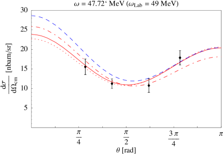
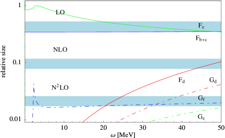
Figure 2: Left: EFT result for the differential cross section fitted to data [20]. Dashed: $\alpha_{0}=\beta_{0}=0$; dot-dashed: $\beta_{0}=0$; dotted: $\alpha_{0}$ and $\beta_{0}$ fitted; solid: $\alpha_{0}$ and $\beta_{0}$ constrained by the Baldin sum rule. Right: Sizes of the (angle averaged) contributions $F_{i}$ and $G_{i}$, normalised to the LO contribution of the seagull term: $|F_{i},G_{i}|/|F_{a}^{(0)}|$. The values assumed for the polarisabilities are $12$ and $5$. The grey bars are meant to guide the eye in determining the size of a contribution in the $Q/\Lambda$ expansion.

The gap between our extraction of the polarisabilities and the $\chi$PT results is well known, see e.g. [11]. It can be traced back to the fact that the Compton scattering data at large angles is systematically more and more enhanced over forward scattering as the photon energy is increased [20, 23]. This favours larger values of $\beta_{0}$.

Although the scarcity of data at low energies is a big hindrance, the comparison of the present calculation to experiment shows that it is quite appropriate to determine neutron scalar polarisabilities from low energy Compton scattering. Our approach uses EFT and hence it is model-independent and allows one to estimate the theoretical accuracy as $\sim 20\%$ for the polarisabilities, assuming higher order contributions are of natural size. Future higher precision experiments e.g. at TUNL in the energy régime $\omega\sim 25-50\;\mathrm{MeV}$ would be most useful. As one can see from Fig. 2, at lower photon energies, the polarisability contributions become smaller than N²LO, while higher energies introduce large theoretical errors since corrections going like $\omega/\Lambda$ are not suppressed sufficiently strong any more. The energy régime proposed is hence an interesting window of opportunity to determine nucleon polarisabilities in a model-independent way without having to deal with pions as explicit degrees of freedom. Small angle scattering data constrains $\alpha_{0}+\beta_{0}$ and hence can serve as a cross check to the Baldin sum rule, whereas backscattering data probes $\alpha_{0}-\beta_{0}$ and hence is needed for a better determination of $\beta_{0}$. In a future publication [14], we will address details of the calculation as well as a more accurate estimate of N³LO effects. The only undetermined operators entering at N³LO are $(C_{E}\vec{E}^{2}+C_{M}\vec{B}^{2})(N^{T}P_{i}N)^{\dagger}(N^{T}P_{i}N)$ with projections $P_{i}$ onto the ${}^{3}S_{1}$ channel. These operators contribute to residual electric and magnetic deuteron polarisabilities, i.e. to those not generated by polarisation of the two nucleons against each other or by polarising the nucleons themselves.

References

- [1] K. W. Rose, B. Zurmühl, P. Rullhusen, M. Ludwig, M. Schumacher, J. Ahrens, A. Zieger, D. Christmann and B. Ziegler: Nucl. Phys. A514, 621 (1990).
- [2] J. Schmiedmayer, P. Riehs, J. A. Harvey and N. W. Hill: Phys. Rev. Lett. 66, 1015 (1991).
- [3] L. Koester, W. Waschkowski, L. V. Mitsyna, G. S. Samosvat, P. Prokofevs and J. Tambergs: Phys. Rev. C51, 3363 (1995).
- [4] B. E. MacGibbon, G. Garino, M. A. Lucas, A. M. Nathan, G. Feldman and B. Dolbilkin: Phys. Rev. C52, 2097 (1995) [nucl-ex/9507001].
- [5] V. Bernard, N. Kaiser and U. G. Meißner: Phys. Rev. Lett. 67, 1515 (1991); Nucl. Phys. B373, 364 (1992); Phys. Lett. B319, 269 (1993) [hep-ph/9309211].
- [6] V. Bernard, N. Kaiser, A. Schmidt and U. G. Meissner: Phys. Lett. B319, 269 (1993) [hep-ph/9309211].
- [7] T. R. Hemmert, B. R. Holstein, J. Kambor and G. Knochlein: Phys. Rev. D57, 5746 (1998) [nucl-th/9709063].
- [8] M. I. Levchuk and A. I. L’vov: Few-Body Syst. Suppl.9, 439 (1995); [nucl-th/0010059].
- [9] M. Weyrauch: Phys. Rev. C41, 880 (1990).
- [10] T. Wilbois, P. Wilhelm and H. Arenhövel: Few-Body Syst. Suppl.9, 263 (1995).
- [11] J. J. Karakowski and G. A. Miller: Phys. Rev. C60, 014001 (1999) [nucl-th/9901018].
- [12] J. W. Chen, H. W. Grießhammer, M. J. Savage and R. P. Springer: Nucl. Phys. A644, 221 (1999) [nucl-th/9806080]; Nucl. Phys. A644, 245 (1999) [nucl-th/9809023].
- [13] S. R. Beane, M. Malheiro, D. R. Phillips and U. van Kolck: Nucl. Phys. A656, 367 (1999) [nucl-th/9905023].
- [14] H. W. Grießhammer and G. Rupak: in preparation.
- [15] J. W. Chen, G. Rupak and M. J. Savage: Nucl. Phys. A653, 386 (1999) [nucl-th/9902056].
- [16] S. R. Beane, P. F. Bedaque, W. C. Haxton, D. R. Phillips and M. J. Savage: “From Hadrons to Nuclei: Crossing the Border”, essay for the Festschrift in honour of Boris Ioffe, to be published as ’Encyclopedia of Analytic QCD’, ed. M. Shifman, World Scientific. [nucl-th/0008064].
- [17] P. F. Bedaque and H. .W. Grießhammer: Nucl. Phys. A671, 357 (2000) [nucl-th/9907077].
- [18] G. Rupak: Nucl. Phys. A678, 405 (2000) [nucl-th/9911018].
- [19] D. R. Phillips, G. Rupak and M. J. Savage: Phys. Lett. B473, 209 (2000) [nucl-th/9908054].
- [20] M. A. Lucas, Ph. D. thesis, University of Illinois at Urbana-Champaign (1994).
- [21] D. Babusci, G. Giordano and G. Matone: Phys. Rev. C57, 291 (1998) [nucl-th/9710017].
- [22] H. W. Grießhammer and T. R. Hemmert: in preparation.
- [23] D. L. Hornidge, B. J. Warkentin, R. Igarashi, J. C. Bergstrom, E. L. Hallin, N. R. Kolb, R. E. Pywell, D. M. Skopik, J. M. Vogt and G. Feldman: Phys. Rev. Lett. 84, 2334 (2000) [nucl-ex/9909015].