Mean–Field Models
and Superheavy Elements

Abstract

We discuss the performance of two widely used nuclear mean-field models, the relativistic mean–field theory (RMF) and the non-relativistic Skyrme–Hartree–Fock approach (SHF), with particular emphasis on the description of superheavy elements (SHE). We provide a short introduction to the SHF and RMF, the relations between these two approaches and the relations to other nuclear structure models, briefly review the basic properties with respect to normal nuclear observables, and finally present and discuss recent results on the binding properties of SHE computed with a broad selection of SHF and RMF parametrisations.

I Introduction

Nuclear structure models are available at various levels of description. There is the macroscopic view in terms of the liquid-drop model (LDM) LDM . The macroscopic-microscopic (mac-mic) method combines the rich phenomenological experience summarised in the LDM with a fine-tuning through shell effects estimated in a properly chosen single-particle potential micmac ; micmac2 . And there is the broad family of self-consistent mean-field approaches (Hartree or Hartree–Fock) employing effective energy functionals on which we will concentrate here. All these models presently enjoy a revival due to a world of new experimental information emerging from the production and measurement of exotic nuclei and new elements. In fact, it is more than three decades ago that speculations on the possible existence of shell-stabilized superheavy elements (SHE) Mosel ; SuperNils have motivated the construction of dedicated heavy-ion accelerators. The production of SHE turned out to be the most tedious task in the field of exotic nuclei. It took about two decades to reach the first island of shell-stabilised deformed SHE in the region of $Z=108$ Dubna ; GSI ; GSI2 . Recent experiments give first evidence for nuclei even closer to the expected island of spherical SHE. The synthesis of the neutron-rich isotopes ${}^{283}112$, ${}^{287-289}114$ Z114 , and ${}^{292}116$ Z116 were reported from Dubna and at Berkeley three $\alpha$-decay chains attributed to the even heavier ${}^{293}118$ were observed Z118 . While earlier superheavy nuclei could be unambiguously identified by their $\alpha$-decay chains leading to already known nuclei, the decay chains of the new-found superheavy nuclei cannot be linked to any known nuclides. The new discoveries still have to be viewed carefully, see the critical discussion in Arm00a . While for the heaviest systems only their mere existence and a few decay properties are established, the first spectroscopic data become available for nuclei at the lower end of the superheavy region, e.g. low-lying states in Rf isotopes from the analysis of $\alpha$-decay fine-structure Hessberger and rotational bands of nuclei around ²⁵⁴No which were found to be stable against fission at least up to $I=16$ Reiter ; Leino . Interpretation of data and planning of future experiments call for a significant refinement in the modeling of SHE. As their mere existence emerges from a delicate balance between the Coulomb instability of the liquid drop against fission and stabilisation through shell effects, SHE provide a demanding testing ground for nuclear structure models, probing all their details. The aim of this review is to examine the performance of current nuclear mean-field models under the particular perspective of SHE. In this context we concentrate on the two most widely used brands, the relativistic mean-field model (RMF) and the non-relativistic Skyrme-Hartree-Fock approach (SHF). We ought to mention that there are also other models like the non-relativistic Gogny force gogny ; gogny2 employing finite-range terms in the interaction, the energy functionals of Fayans et al. fayans which are similar to SHF but use variants of density dependence and pairing interaction, or the point-coupling variant of the RMF madland which can be viewed as the relativistic analogue of the Skyrme interaction. As none of these was widely used for the calculation of SHE so far we omit them from our discussion.

The paper is outlined as follows: Section II provides the theoretical background of the RMF and SHF, tries to establish the relation between these two approaches and the relations to the more macroscopic methods (LDM and mic-mac). Section III presents and discusses a selection of typical results.

II Framework

II.1 Mean-field models in the hierarchy of approaches

Self-consistent mean-field models are intermediate between the fully microscopic many-body theories as, e.g., Brückner–Hartree–Fock (BHF) BHF and semi-classical models as the mac-mic approach micmac ; micmac2 . The microscopic approaches have made considerable progress over the past decades BHF ; HenPan , yet the actual precision in describing nuclear properties is still limited. Moreover, application to finite nuclei is extremely expensive. Thus fully microscopic methods are presently not used for large-scale nuclear structure calculations. They provide, however, useful guidelines for the construction of effective mean-field theories Tmatexp .

On the other side are the macroscopic approaches which are inspired by the idea that the nucleus is a drop of nuclear liquid, giving rise to the liquid-drop model (LDM) and the more refined droplet model droplet . With a mix of intuition and systematic expansion one can write down the corresponding energy functional even including finite-range effects of the nuclear interaction FRDM ; FY . There remain a good handful of free parameters, as e.g. the coefficients for volume energy $a_{\rm vol}=E/A$, symmetry energy $a_{\rm sym}$, incompressibility $K_{\infty}$, or surface energy $a_{\rm surf}$. These have to be adjusted to a multitude of nuclear bulk properties such that modern droplet parametrisations deliver an excellent description of average trends LDM . Actual nuclei, however, deviate from the average due to quantum shell effects, so that shell corrections are added, which are related to the level density near the Fermi surface and can be computed from a well tuned nuclear single-particle potential. Macroscopic energy plus shell corrections constitute the mac-mic approach which is enormously successful in reproducing the systematics of known nuclear binding energies micmac ; micmac2 ; FRDM ; FY . One has to admit, though, that the mac-mic method relies strongly on phenomenological input. This induces uncertainties when extrapolating to exotic nuclei. Particularly uncertain is the extrapolation of the single-particle potential because this is not determined self-consistently but added as an independent piece of information.

Self-consistent mean-field models do one big step towards a microscopic description of nuclei. They produce the appropriate single-particle potential corresponding to the actual density distribution for a given nucleus. Still, they cannot be handled as an ab initio treatment because the genuine nuclear interaction induces huge short-range correlations. Self-consistent mean-field models deal with effective energy functionals. The concept has much in common with the successful density-functional theory for electronic systems GD90 ; Petkov . Taking up the notion from there, we can speak of nuclear Kohn-Sham models as synonym for mean-field models. The difference is, however, that electronic correlations are well under control and that reliable electronic energy-density functionals can be derived ab initio. Nuclear many-body theories, as discussed above, have not yet reached sufficient descriptive power to serve as immediate input for effective mean-field models, but serve as motivation and source for the basic features of the mean-field approach. This sets the framework, the actual energy functionals are then constructed by systematic expansion considering symmetries Dob96a , their parameters are adjusted phenomenologically. (For a recent review on nuclear correlations and their relation to effective mean-field theories see Rei94a .)

The connection between self-consistent mean-field models and mac-mic approaches is much better developed. There are several attempts from either side. The ETFSI approach starts from SHF and derives an effective mac-mic model by virtue of a semi-classical expansion ETFSI . From the macroscopic side there is an attempt to induce more self-consistency by virtue of a Thomas-Fermi approach TFmyers . The investigation of these links is useful to gain more insight into the crucial constituents of either models.

II.2 Skyrme–Hartree–Fock model

The concept of an effective interaction for mean-field calculations can be justified within many-body theories. For example, the $T$-matrix in BHF is the actual effective force for the underlying mean field. It was a formal $T$-matrix expansion Tmatexp which gave theoretical support to the first working self-consistent model Skfirst using an effective interaction introduced much earlier by T. H. R. Skyrme skyrme ; skyrmeLS . The original idea was that a convenient-to-use effective interaction can be obtained from a momentum-space expansion of any finite-range interaction which leads to a zero-range force plus momentum-dependent terms. A density dependence has to be added to incorporate many-body correlations in an effective way (note that the $T$ matrix depends strongly on density) and, last not least, a (zero-range) spin-orbit force skyrmeLS is added to account for the strong spin-orbit splitting in nuclei.

This concept has an intimate relation to energy-density functionals. The energy expectation value of such an effective interaction is precisely a functional of the local density. Thus the well developed density-functional theory GD90 adds support for SHF. We present here the SHF functional complemented by an obvious graphical illustration:

The first two columns parametrise a density functional marked $F(\rho)$. Note the distinction between total (isoscalar) density $\rho=\rho_{\rm p}+\rho_{\rm n}$ and isovector density $\tilde{\rho}=\rho_{\rm p}-\rho_{\rm n}$, and similarly for the kinetic density $\tau$ and the spin-orbit current ${\bf J}$. The leading term is the two-body interaction $\propto\rho^{2}$. It is attractive in the isoscalar channel and repulsive for the isovector part, just as the genuine two-body force is. The necessary density-dependent interaction is parametrised in the next term, for traditional reason in the form of an extra $\rho^{\alpha}$. These two terms together set up a local-density functional which is represented graphically as $F(\rho)$ where a heavy dot with an appended circle stands for the density. That density functional allows already to fix all relevant nuclear bulk properties. Finite systems require a fine-tuning of surface properties which is achieved by the gradient correction term. They are represented graphically by the right-left arrow atop the $\rho*\rho$ symbol. Moreover, the strong dressing of nucleons in matter calls for an effective mass $m^{*}/m<1$ effmass which can be achieved by the kinetic correction term $\propto\rho\tau$ where $\tau=\sum_{\alpha}|\nabla\varphi_{\alpha}|^{2}$. This term requires derivatives within the density summation which is indicated by an up-down arrow in one of the two densities. Last but not least, a strong spin-orbit splitting is crucial for a correct description of single-particle spectra and shell closures lsfirst . This is guaranteed by the spin-orbit term $\propto\rho\nabla\cdot{\bf J}$ where the spin-orbit current is indicated graphically by a circle with arrow around the density-dot. Note that each term comes twice, once in an isoscalar form and another time in an analogous isovector form.

The nice feature of the Skyrme functional is that each term can be related to a corresponding bulk property (or LDM feature). This is indicated in the last two lines of the above sketch. The two isoscalar density-dependent parts together are related to bulk binding $E/A$, equilibrium density $\rho_{0}$, and incompressibility $K_{\infty}$. The isovector part complements this by the symmetry-energy coefficient $a_{\rm sym}$ and its derivative $\partial_{\rho}\,a_{\rm sym}$. The gradient corrections relate naturally to the isoscalar and isovector surface-energy coefficients. The kinetic terms adjust the isoscalar effective mass $m^{*}/m$ and the isovector effective mass $m^{\prime}{}^{*}$. The latter modifies the Thomas-Reiche-Kuhn sum rule RingSchuck by an enhancement factor $1+\kappa_{\rm sumrule}=m/m^{\prime}{}^{*}$ and one often parametrises $m^{\prime}{}^{*}$ in terms of this enhancement factor, see e.g. SLyx . No bulk property can be associated directly with the spin-orbit term. This term is related to the shell structure, i.e. to the single-particle spectrum, of finite nuclei. What looks here like a quickly drawn and superficial analogy to the LDM, has indeed deep theoretical foundations. One can, in fact, derive the mic-mac method from SHF by virtue of semi-classical expansions SHF2micmac .

There is a subtle difference between the force concept and the energy functional concept which concerns the spin-orbit force. Derivation of the energy functional from a Skyrme force yields (usually small) extra terms ${\bf J}^{2}$ and $\tilde{\bf J}^{2}$ which emerge from the exchange part of the kinetic terms $\propto\rho\tau$ or $\tilde{\rho}\tilde{\tau}$. Some Skyrme parametrisations include these terms, some do not. We will specify that later when presenting the parametrisations. The actual Hartree-Fock (or Kohn-Sham) equations are derived variationally from the given energy functional, see e.g. SkIx ; RPAnucl .

II.3 Relativistic mean-field model

The history of the RMF has similarities to SHF. After an early first conjecture duerr , it was only in the seventies that this model was lifted to a competitive mean-field model RMF1 ; RMF2 . The starting point is, at first glance, different from SHF. RMF is conceived as a relativistic theory of interacting nucleonic and mesonic fields. The mesonic fields are approximated to mean fields (real-number fields rather than field operators), a feature which is reflected in the name RMF. Moreover, the anti-particle contributions in the Dirac fields for the nucleons are suppressed (“no–sea” approximation). Again, the mean-field approximation is not valid in connection with the true physical meson fields. The meson fields of the RMF are effective fields at the same level as the forces in SHF are effective forces. The RMF is the relativistic cousin of SHF, and the same strategy applies: relativistic BHF is still not precise enough to allow an ab initio derivation of the RMF; the model is postulated from a mix of intuition and theoretical guidelines with the parameters to be fixed phenomenologically.

The RMF is usually formulated in terms of an effective Lagrangian, as any relativistic theory. For stationary problems it can be mapped to an energy functional Schmid . We discuss it here in terms of an effective energy functional and we confine ourselves to a graphical presentation because the RMF is well documented in several reviews Rei89 ; Ser92a ; Rin96a . The RMF functional can be sketched as follows:

The ansatz looks at first glance conceptually even simpler than that of SHF. One merely writes down the basic nucleon-meson couplings RMF1 . The mesons can be characterised by their internal quantum numbers. Scalar and vector fields are taken into account (the most famous pion field does not contribute in Hartree approximation because there is no finite pseudo-scalar density in the ground state). For the isovector part, one employs only the vector field associated with the $\rho$ meson. The isovector-scalar field, the $\delta$ meson, should appear at the same level (and plays a role, indeed, in the nucleon-nucleon force). It can be omitted for purely phenomenological reasons because it does not improve the performance of the model when included. But a simple series of meson-nucleon couplings does not suffice to deliver a high-precision model. We know from microscopic theory that the effective interaction needs density dependence to effectively incorporate many-body correlations. Such had been introduced into the RMF via non-linear terms (cubic and quartic) in the scalar meson field RMF2 , as indicated by the second line in the above sketch. This leads to a model with the same descriptive power as SHF Rei89 ; Ser92a ; Rin96a . This choice to introduce density-dependence was originally motivated by the aim to maintain renormalisibility of the theory. This is not a very stringent condition in connection with an effective mean-field theory which incorporates many-body effects, but the ansatz delivers an empirically well-working scheme and thus there was little pressure for modifications, for exceptions and variants of the modeling see PL40 ; TM1 .

At first glance, the RMF functional looks quite different from SHF, and indeed, the pieces have been put together in a different fashion. The concept of the RMF seems to emerge naturally from a field theoretical perspective whereas the many-body aspects are not so transparent. These had been more obvious in SHF, particularly the relation to nuclear bulk properties, but it is possible to draw straight connections from RMF to SHF. These can be established by considering the non-relativistic and zero–range limit of RMF Rei89 ; thies . It can be sketched as follows:

The left upper two diagrams summarise the RMF from the previous sketch. The right upper box indicates the two independent steps of expansion: a $v/c$ expansion of the scalar density and a gradient expansion of the meson propagator. The scalar density delivers as leading term the normal density (zero component of vector density) and as $v/c$ corrections the kinetic-energy density $\tau$ as well as the divergence of the spin-orbit current $\nabla\cdot{\bf J}$. The finite range of the mesons is expanded as leading zero-range coupling and gradient correction. Inserting these approximations yields the functional as represented by the diagrams in the second line of the sketch. It looks almost identical to the Skyrme functional. The interpretation in terms of bulk properties then proceeds as in case of SHF. It is repeated here for the sake of completeness. There is one aspect, however, which is very hard to map: it is the form of the density dependence. The mechanism in the RMF goes through non-linear meson coupling and is much different from the SHF with its straightforward expansion in powers of density $\rho$. A thorough comparison of the density dependences is still a task for future research. As in case of the SHF, we skip a detailed derivation of the coupled field equations and refer the reader to Rei89 ; Ser92a ; Rin96a .

II.4 Further ingredients

The above two subsections have outlined the main body of SHF and RMF. There are several further details which are handled similarly in both approaches. The direct part of the Coulomb interaction is given by the standard expression $E_{\rm coul}=\frac{1}{2}\int\!d^{3}r\,d^{3}r^{\prime}\;\rho_{c}({\bf r})\,|{\bf r}-{\bf r}^{\prime}|^{-1}\rho_{c}({\bf r}^{\prime})$ where the charge density $\rho_{c}$ is usually replaced by the mere proton density $\rho_{c}\rightarrow\rho_{p}$ omitting substructure and finite size of the nucleons. While the RMF includes the direct term only, all modern SHF parameterizations employ the Slater approximation for the exchange term $E_{\rm coul,ex}=\frac{3}{4}e^{2}\int\!d^{3}r\,\rho_{p}^{4/3}({\bf r})$ GD90 .

A further crucial ingredient are pairing correlations. There are several recipes in the literature differing in the variational principle used, the correction for the particle-number uncertainty of the BCS state and the effective pairing interaction. Nowadays, for the latter a zero-range two-body pairing force $V_{\rm pair}=V_{0,p/n}\delta({\bf r}_{1}-{\bf r}_{2})$ with separately adjustable strengths for protons and neutrons is most widely used. For most calculations reported here the matrix elements of this force are used in the BCS equations (as approximation to Hartree–Fock–Bogoliubov). For a recent discussion of this and competing recipes see gappaper and references therein.

The mean field localises the nucleus in space. This violates translation invariance. Center-of-mass projection restores that symmetry RingSchuck . It turns out that a second-order estimate for the center-of-mass correction is fully sufficient. The correction is performed by subtracting $E_{\rm cm}^{\rm(2)}=\langle\hat{P}_{\rm cm}^{2}\rangle/2mA$ from the calculated binding energy where $m$ is the nucleon mass and $A$ the mass number, see cmpaper for details. The term is usually subtracted a posteriori to circumvent two-body terms in the mean-field equation. For some parameterizations this is even simplified further. One approach is to use the harmonic oscillator estimate $E_{\rm cm}^{\rm(est)}=\frac{3}{4}41.5\,{\rm MeV}A^{-1/3}$, another to use only the diagonal part of $\hat{P}_{\rm cm}^{2}$, i.e. $E_{\rm cm}^{\rm(diag)}=\sum_{i}\langle\hat{p}_{i}^{2}\rangle/2mA$. The latter recipe leads to a simple renormalisation of the nucleon mass $1/m\rightarrow 1/m\times(1-1/A)$ and is usually included in the variational equations. Different groups are using different recipes for the center-of-mass correction and thus one has to keep track which recipe is employed with a given parametrisation.

In fact, center-of-mass correction is already one step, although the most trivial, beyond the mean-field approach. There are many other correlation effects possibly to be considered, particle-number projection, angular-momentum projection in case of deformed nuclei, vibrational corrections. These aspects are being investigated intensively at present. Here we stay at the strict mean-field level (plus c.m. correction).

II.5 Parametrisations

As already mentioned above, nuclear many-body theory is not yet precise enough to allow an ab initio derivation of the effective energy functionals for SHF or RMF from nucleon-nucleon interactions. Theory, with a spark of intuition, sets the frame and defines the form of the functional. The remaining free parameters have to be adjusted phenomenologically. Different groups have different biases in selecting the observables to which a force should be fitted. One usually restricts the fits to a few spherical nuclei with at least one magic nucleon number (an exception is a recent large-scale fit to all known nuclear masses pearstond ). All fits take care of binding energy $E_{B}$ and r.m.s. charge radii $r$. From then on, different tracks are pursued. SHF fits invoke extra information on spin-orbit splittings. RMF generally does not need that because the spin-orbit interaction is a relativistic effect that emerges naturally from relativistic models. Some groups add information on nuclear matter, some even on neutron matter. Some groups give a weight to isovector trends. Others make a point to include more information from the electromagnetic formfactor, in terms of a diffraction radius and surface thickness Fri86a . A detailed discussion of a fitting strategy can be found, e.g., in SkIx ; Rei89 ; Fri86a .

In view of these different prejudices entering the determination of a force, it is no surprise that there exists a world of different parametrisations for SHF as well as RMF. We confine the discussion to a few well adjusted and typical sets. For SHF we consider the parametrisations ${\rm SkM}^{*}$ SkM* , SkP SkP , SkT6 Tx , Z_σ Fri86a , SkI3, SkI4 SkIx , and SLy6 SLyx . The forces SkM^∗, SkT6, SkP, and Z_σ can be called the second generation forces which emerged in the mid eighties and which delivered for the first time a well equilibrated high-precision description of nuclear ground states. The force ${\rm SkM}^{*}$ was the first to deliver acceptable incompressibility and fission properties. It also provides a fairly good description of surface thickness although this type of data was not fitted explicitly. The force SkT6 is a fit with constraint on $m^{*}/m=1$. It did take into account the nuclear surface energy and thus also provides a satisfying surface thickness ($\equiv$ electromagnetic formfactor). The force SkP uses effective mass $m^{*}/m=1$ and is designed to allow a self-consistent treatment of pairing. We will skip this pairing feature and use an appropriately adjusted delta pairing force. The force Z_σ stems from a least-squares fit including diffraction radius and surface thickness but without any reference to pseudo-data from nuclear matter. The forces SLy6, SkI3, and SkI4 have been developed in the nineties. They take care of new data (e.g. from exotic nuclei) and new aspects. The force SLy6 stems from a recent attempt to cover properties of pure neutron matter together with normal nuclear ground state properties, sacrificing the quality of surface thickness somewhat to achieve this. All Skyrme forces up to here use the spin-orbit coupling in the particular combination $3\rho\nabla\cdot{\bf J}+\tilde{\rho}\nabla\cdot\tilde{\bf J}$ which is dictated by deriving the spin-orbit energy from a two-body zero-range spin-orbit force skyrmeLS . The forces SkI3/4 employ a spin-orbit force with isovector freedom to simulate the relativistic spin-orbit structure. SkI3 contains a fixed isovector part $\tilde{b}_{4}=0$ analogous to the RMF, whereas SkI4 is adjusted allow free variation $b_{4}\neq 3\tilde{b}_{4}$ of the isovector spin-orbit force. The modified spin-orbit force was introduced because no conventional SHF force was able to reproduce the isotope shifts of the m.s. radii in heavy Pb isotopes, see SkIx and references cited therein. The isovector-modified spin-orbit force in SkI3 and SkI4 solves this problem. It then has, of course, a strong effect on the spectral distribution in heavy nuclei and thus for the predictions of SHE.

For the RMF we consider the parametrisations NL–Z NLZ , NL3 NL3 and TM1 TM1 . The force NL–Z comes from fits with the choice of observables quite similar to those of SkI3 and SkI4, with in particular the charge formfactor taken care of. NL3 is fitted without looking at the formfactor but more emphasis on the isovector trends. TM1 is an extended version of the RMF including a quartic non-linear self-coupling of the isoscalar-vector field.

Each parametrisation is complemented by Coulomb, pairing and center-of-mass correction as outlined in section II.4. The pairing strengths need to be adjusted separately to comply with the level density of the force. Table 1 provides the actually used pairing strengths. The table indicates also the type of center-of-mass correction used.

Table 1: Proton and neutron pairings strengths (in [MeV fm³]) and center-of-mass recipe for the parametrisations used in this paper. For details of the adjustment of the pairing strengths and the cutoff used see gappaper .

	SkM∗	SkT6	SkP	Zσ	SLy6	SkI3	SkI4	NL-Z	NL3	TM1
$V_{0,p}$	$-292$	$-256$	$-265$	$-290$	$-320$	$-350$	$-323$	$-351$	$-342$	$-327$
$V_{0,n}$	$-276$	$-250$	$-241$	$-269$	$-308$	$-340$	$-310$	$-349$	$-329$	$-323$
c.m.	$E_{\rm cm}^{\rm(diag)}$	$E_{\rm cm}^{\rm(diag)}$	$E_{\rm cm}^{\rm(diag)}$	$E_{\rm cm}^{\rm(2)}$	$E_{\rm cm}^{\rm(2)}$	$E_{\rm cm}^{\rm(2)}$	$E_{\rm cm}^{\rm(2)}$	$E_{\rm cm}^{\rm(2)}$	$E_{\rm cm}^{\rm(est)}$	$E_{\rm cm}^{\rm(est)}$

III Results and discussion

III.1 Basic properties

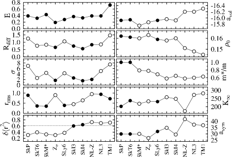
Figure 1: Left panels: relative errors (in $\%$) of key observables of finite nuclei for the selection of forces: binding energy $E$, diffraction radius $R_{\rm diff}$, surface thickness $\sigma$, and r.m.s. radius $r_{\rm rms}$. The lowest left panel shows the isotopic shift of the m.s. radius in ²¹⁴Pb, $\delta\langle r^{2}\rangle=r^{2}(^{214}{\rm Pb})-r^{2}(^{208}{\rm Pb})$, in units of ${\rm fm}^{2}$. Its experimental value is indicated by a horizontal dotted line. Right panels: properties of the model system of infinite homogeneous symmetric spin-saturated nuclear matter: volume-energy coefficient $a_{\rm vol}$ (in MeV), equilibrium density $\rho_{0}$ (in fm^-3), (isoscalar) effective mass $m^{*}/m$ (dimensionless), incompressibility $K_{\infty}$ (in MeV), and symmetry-energy coefficient $a_{\rm sym}$ (in MeV). Full symbols denote quantities that were used in the fit of the particular effective interaction, while open symbols represent predictions.

Before coming to a discussion of SHE we review briefly the basic properties of the various parametrisations, their performance with respect to normal nuclei and their nuclear matter properties (which are equivalent to the coefficients of the LDM expansion). They are summarised in Fig. 1. Note that only a sub-set of these data are used in actual fits. The left panels deal with finite nuclei. They show the r.m.s. errors of the basic ground-state properties (relative errors in $\%$). Note that diffraction radius and surface thickness are key quantities determining the electromagnetic formfactor Fri86a . For the nuclei discussed here $R_{\rm diff}$, $\sigma$ and $r_{\rm rms}$ are linked by the Helm model in such a way that only two values are independent FriVoe . The lowest panel adds a more specific piece of information: the isotopic shift in heavy Pb isotopes. The energy (uppermost panel) is very well reproduced. All chosen forces have an error of only $0.4\%$ or below. More differences are seen concerning the reproduction of radii and surface thicknesses. The correlation is obvious: quantities which had been included in the adjustment (full dots) are usually well reproduced. Those which had not been fitted tend to show larger errors. Exceptions from the rule to some extent are SkT6 and SkM^∗ which yield acceptable $R_{\rm diff}$ and $\sigma$ without having fitted them. Both forces, however, include a fitted surface energy which is related to reasonable surface thickness Fri86a . A less positive exception is the comparatively large error in $r_{\rm rms}$ for NL3, which includes this observable in the fit, but the other RMF forces have similar problems with $r_{\rm rms}$. It seems that this is a principal problem of the RMF in its present form. It could be related to the somewhat curious form of shaping the density dependence in that approach. After all, one can conclude that the error in radii, $R_{\rm diff}$ or $r_{\rm rms}$, is certainly below $1\%$, often half of that. Surface thicknesses $\sigma$ can be reproduced within $2\%$ if used in the fit; moreover, $\sigma$ gives a handle on the surface tension (and subsequently on good fission barriers SkM* ; cmpaper ). The lowest right panel in Fig. 1 shows the isotopic shift in heavy Pb isotopes. It is obvious that all conventional Skyrme forces (i.e. those with $b_{4}=\tilde{b}_{4}$) fall short of the experimental value of $\delta\langle r^{2}\rangle=r^{2}(^{214}{\rm Pb})-r^{2}(^{208}{\rm Pb})=0.6\,{\rm fm}^{2}$. All RMF forces hit that value very well as a prediction. It was worked out that this is due to the particular form of the spin-orbit force in the RMF SkIx ; Ringls . Extending the SHF to allow for $b_{4}\neq\tilde{b}_{4}$ yields an equally good reproduction of these isotopic shifts, see SkI3 and SkI4 in Fig. 1. But the values need to be included as fit data because the spin-orbit force is added “by hand” in SHF whereas it is an intrinsic feature of the nucleonic Dirac equation in RMF.

The right panels of Fig. 1 show nuclear matter properties. There is general agreement about the volume energy, although the RMF forces seem to prefer slightly smaller values. The equilibrium density is almost the same for all SHF forces while RMF again prefers slightly smaller values. This systematic difference in extrapolation to nuclear matter is most probably related to the very different way in which the density-dependence is modeled in SHF and RMF. A thorough study of those effects is still lacking.

The effective mass shows a clear trend to values lower than one. It is, however, a rather vaguely fixed property. For example, SkT6 has fixed $m^{*}/m=1$ and is still able to provide good overall quality (see right panels). It is said that fits which concentrate on binding energies automatically prefer $m^{*}/m=1$ pearstond . On the other hand, fits which include the formfactor ($R_{\rm diff}$ and $\sigma$) prefer lower $m^{*}/m$. And the RMF always prefers particularly low values. It is yet an open point what the best value for $m^{*}/m$ should be for nuclear mean-field models. Exotic nuclei, and particularly SHE, may help towards an answer.

Concerning the incompressibility $K_{\infty}$, the SHF forces almost all gather nicely around the generally accepted value of $230\,{\rm MeV}$ incomp , SkP being an exception with a rather low value of $K_{\infty}$. The RMF forces make quite different predictions. NL-Z produces too low $K_{\infty}$, which results from the fit, while NL3 comes up with a rather large value, which is to some extent a bias entering the adjustment. The actual number is probably at the upper edge of presently accepted values. A similarly large value is produced by TM1.

The largest variations are seen for the asymmetry energy $a_{\rm sym}$. The LDM predicts values around $30\,{\rm MeV}$. Indeed, most SHF forces reproduce that nicely, with the exception of SkI3 which comes out too high and Z_σ which yields a somewhat low value, but the RMF forces generally yield a very large value for $a_{\rm sym}$. One then wonders what the properties of the isovector dipole giant resonance might be. It turns out that its position depends not only on $a_{\rm sym}$ but also on the isovector effective mass, or sum rule enhancement factor $\kappa$, respectively. Most Skyrme forces have rather low $\kappa\approx 0\!-\!0.25$, yielding correct resonance frequencies for $a_{\rm sym}\approx 30\,{\rm MeV}$. The RMF forces have much larger $\kappa\approx 0.75$ and here the value $a_{\rm sym}\approx 40\,{\rm MeV}$ is appropriate. For a detailed discussion of these somewhat surprising interconnections see varenna . It remains that there is a substantial difference between SHF and RMF in that respect. The reasons are as yet unclear; it is probably again caused by the different form of density-dependence.

III.2 Binding Energies of Superheavy Nuclei

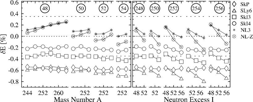
Figure 2: Relative error on binding energies $\delta E=(E_{\rm calc}-E_{\rm expt})/E_{\rm expt}$, of even-even superheavy nuclei for the selection of forces drawn versus mass number $A=N+Z$ for constant $I=N-Z$ (left panel) and versus $I$ for constant $A$ (right panel). Note that the left panel corresponds to $\alpha$–decay chains. The quality margin of $0.35\;\%$ which was the achieved average error for normal nuclei is indicated by dotted lines. See Ref. Bue98a for a discussion of the theoretical uncertainties. Data taken from Bue98a ; dubna .

We now proceed to the discussion of SHE. The first feature to look at is, of course, the binding energy. Fig. 2 shows the relative error on binding energies $\delta E$ for a selection of already known SHE. One sees at first glance, that the errors stretch out towards under-binding. The RMF forces remain very well within the desired error bands. The two SHF forces with extended spin-orbit splitting also stay just within the bounds, and all conventional SHF forces fall below the $0.35\;\%$ margin. This is most probably not caused by the underlying bulk properties but related to shell effects. Note that Fig. 2 presents the same data in two different fashions to disentangle different trends in the error stemming from the isoscalar ($I=$ const.) and isovector ($A=$ const) channel of the interaction dubna . We look first at the left panel where the trends with $A$ are drawn. It is gratifying to see that all SHF forces basically follow a horizontal line which implies that the isoscalar bulk properties are described correctly. The RMF lines, however, have visible slopes, showing that the trends with $A$ are not perfectly reproduced. Such a feature had already been hinted at in Fig. 1 where the volume parameters $a_{\rm vol}$ and $\rho_{0}$ from the RMF differed from those of SHF and from the typical LDM values. This again most probably indicates a deficiency of the density-dependence in RMF.

The right panel of Fig. 2 displays the isovector trends. Clearly almost no force hits these trends correctly. SkP shows the most horizontal lines and thus seems to incorporate some correct isovector features. It is, on the other hand, a strange surprise that SLy6 deviates so much from the experimental isovector trends. This force was intended to perform particularly well in the isovector channel. The feature has yet to be fully understood. Keeping in mind that the actual trends are a mix of isovector bulk properties and shell effects it is most probable that the shell effects cause these deviations. SkI3 has as bad trends as SLy6 while SkI4 performs a bit better. This again is an accident because these trends had not been included in the fit. The RMF forces also fail with respect to isovector trends, The force NL3 performing a bit better than NL-Z, possibly because isovector trends of binding energies had been included in the fit. It is even more surprising that NL3 does not perform better. There are still open problems with a proper parametrisation of the isovector channel in the RMF. Remembering that there is only one isovector field taken into account, one would like to also incorporate the scalar-isovector field (the $\delta$ meson) to achieve a better isovector performance in the RMF, but this channel probably needs non-linear couplings because a simple linear ansatz did not lead to improvements RutzDiss .

All these results on this apparently innocuous observable binding energy hint that new information from SHE sheds new light on mean-field models. A thorough study of the reasons for underbinding and unresolved trends has yet to come and will certainly help to deduce new constraints on the parametrisations.

III.3 Shell Effects

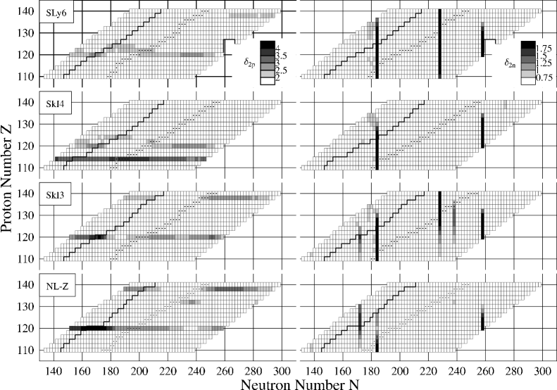
Figure 3: Grey scale plots of two-proton shell gaps $\delta_{\rm 2p}$ (left column) and two-neutron shell gaps $\delta_{\rm 2n}$ (right column) in the $N$–$Z$ plane for spherical configurations calculated with the effective interactions as indicated. The assignment of scales differs for protons and neutrons, see the uppermost boxes where the scales are indicated in units of MeV. The most bound nuclei in each isobaric chain and the two-proton drip-line are emphasized. Data taken from firstSH .

Shell effects are constitutive for the existence of SHE and they play a crucial role in determining the actual stability against fission. It is thus worthwhile to have a closer look at shell effects. A prominent feature is the occurrence of shell closures or magic numbers, respectively, in the single-particle spectrum. One way to characterise them is to examine the two-nucleon separation energies, e.g. $S_{2n}=E(Z,N-2)-E(Z,N)$. They display a sudden drop at shell closures because it is easier to remove nucleons from the next open shell (the former valence shell). The size of the step is a measure for the “magicity” of the shell closure. It is given by the two-nucleon shell gaps, e.g. for the neutrons

$$\delta_{\rm 2n}(Z,N) = S_{\rm 2n}(Z,N)-S_{\rm 2n}(Z,N+2)$$ (1)

$$= E(Z,N+2)-2E(Z,N)+E(Z,N-2)$$

and similarly for the protons. This quantity is a way to access the gap between last occupied and first unoccupied single-particle states, see e.g. Ben99a . Peaks in $\delta_{2p}$ or $\delta_{2n}$ indicate a shell closure. Fig. 3 shows proton and neutron shell gaps for a large range of SHE and for a subselection of forces. It is done for simplicity with spherical calculations. This suffices when searching for spherical shell closures. Deformation might change the picture in details and adds deformed shell closures, e.g. $N=162$ or $Z=108$, see Bue98a . The left panels show $\delta_{2p}$. The dark horizontal stripes thus indicate the closed proton shells. The right panels show $\delta_{2n}$, the dark vertical stripes there stay for closed neutron shells. The different forces show quite different patterns. This holds particularly for the proton shell closures. The RMF force NL–Z and the most RMF-like SHF force SkI3 predict a magic $Z=120$ whereas SkI4 prefers $Z=114$ and SkP shows no pronounced proton shell closures at all. For the neutrons, all SHF forces predict a $N=184$ shell while RMF prefers $N=172$. That is not mutually exclusive. Several forces, SHF and RMF, have both closures.

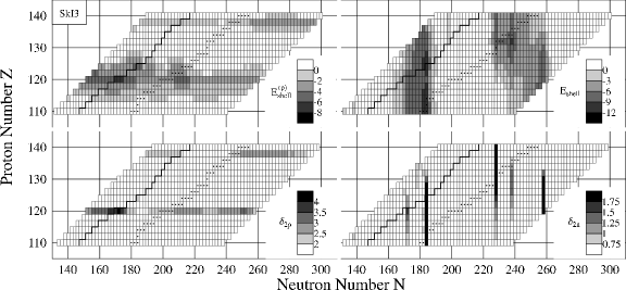
Figure 4: Grey-scale plots of the shell correction energies $E_{\rm shell}^{(q)}$ (upper panels) and the two-nucleon shell gaps $\delta_{2q}$ (lower panels) for protons (left panels) and neutrons (right panels) calculated with SkI3 for spherical shapes. Data taken from firstSH ; newshelcor .

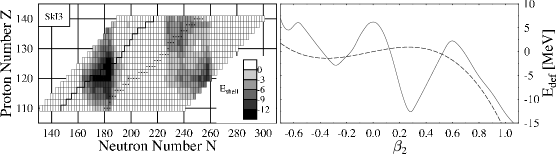
Figure 5: Grey-scale plots of the total shell correction energy $E_{\rm shell}=E_{\rm shell}^{\rm(p)}+E_{\rm shell}^{\rm(n)}$ calculated with SkI3 for spherical shapes (left panel) and schematic plot of the shell stabilization of a superheavy nucleus. (right panel). Data taken from newshelcor .

The shell gaps $\delta_{2q}$ are very useful when searching shell closures, but they are not directly related to the “shell effect” that stabilizes SHE against Coulomb fission. This quantity is provided by the shell correction energy

$$E_{\rm shell}=\sum_{\alpha}\varepsilon_{\alpha}-\int\!{\rm d}\varepsilon\;\tilde{g}(\varepsilon)\quad.$$ (2)

High level density around the Fermi surface yields positive $E_{\rm shell}$ which corresponds to reduced binding. Smaller–than–average level density, in turn, corresponds to negative $E_{\rm shell}$, i.e. extra binding from shell effects LDM ; micmac ; micmac2 . Fig. 4 shows an example of the individual shell correction of protons and neutrons in comparison with the two-nucleon shell gaps $\delta_{2q}$. While in mac–mic models the shell correction is an constitutive part of the calculation of the binding energy, the values presented here are a posteriori analysed from the actual single-particle spectra of fully self-consistent calculations as a measure of the shell effect shelcor . Maximum (negative) values of the shell corrections coincide with the peaks in $\delta_{2q}$, but there is also a significant difference. While the two-nucleon shell gaps show isolated peaks, the shell corrections appear as rather broad valleys of shell stabilised nuclei. The valley is broader than that around magic shells for normal nuclei. The stabilizing effect of the shell correction is given by the sum of the shell corrections for proton and neutrons. The mechanism is sketched in the right panel of Fig. 5. The dashed line indicates the smooth deformation energy curve corresponding to the LDM background. It is repulsive for SHE which means that they all would be fission-unstable in a LDM world. The full line has the shell corrections added. They oscillate with deformation and this generates minima which are stabilised against fission. The amplitude of the oscillations corresponds to the height of the fission barrier. Thus the depth of the shell-correction valley is a rough measure for fission stability. The total shell correction energy is given in the left panel of Fig. 5. There emerges a broad region of shell stabilised SHE. The positive aspect of these findings is that one has good chances to hit long-living SHE in a variety of entrance channels. The negative aspect is that the quest for doubly-magic SHE is misleading. Magicity is not very pronounced out there, a feature which was already seen in mac-mic models FY . The crucial features for SHE are large shell corrections, and these exist; even better, they appear for a broad range of $Z$ and $N$ which makes the search for SHE in some sense comfortable.

III.4 Single–particle structure

Both previous sections have pointed out signatures of shell effects. In this section we sketch the actual single-particle spectra of SHE. The left panel of Fig. 6 shows the proton levels near the Fermi surface for $Z=120$ and varying $N$. The overall trend is obvious: proton levels become more deeply bound with increasing $N$, but note the change of the gap at $Z=120$ along the isotopic chain which is coupled to the magic neutron number; a slight shift of the single-particle energies destroys the $Z=120$ around $N=184$. This illustrates the same effect seen in the $\delta_{\rm 2p}$ in Fig. 3. It is a typical self-consistency effect not seen in earlier mac-mic calculations caused by the strong coupling of bulk properties and single-particle structure. We will come back to that in Section III.5. The right lower panel of Fig. 6 tries to visualize the competition between the $Z=114$ and $Z=120$ shell.

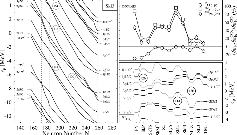
Figure 6: Left panel: Single-proton levels in the vicinity of the Fermi energy for the chain of $Z=120$ isotopes as predicted by SkI3 plotted versus the neutron number. The dotted vertical lines indicate the spherical magic neutron numbers $N=172$, $N=184$ and $N=258$ predicted by SkI3. Right top panel: Relative error of the spin-orbit splitting of selected proton states in the doubly-magic nuclei as indicated. Experimental data taken from NUDAT except the proton $2d$ splitting in ¹³²Sn taken from Sb133 . Note that earlier papers Ben99a have used the larger value of this splitting taken from NUDAT . FY denotes the Folded–Yukawa single-particle potential widely used in mac–mic models FRDM . Right bottom panel: Single-nucleon spectra for ${}^{292}120$ at spherical shape calculated with the interactions as indicated Left: proton spectra. Right: neutron spectra. Note that this nucleus is deformed for most SHF interactions. Data taken from Ben99a .

The lower right panel of 6 displays the proton spectra for ${}^{192}120$. Most interactions predict the same level-ordering in the superheavy region, the different bias on 114 and 120 among the forces found in Fig 3 is related to slight changes in the relative distances of the levels. The reason for this behaviour is clearly apparent: the $Z=114$ shell corresponds to large spin-orbit splitting of the $2f$ proton levels, while the $Z=120$ shell requires small $2f$ splitting. Because the self-consistency makes the level scheme depend strongly on $Z$ and $N$ (cf. the left panel of Fig. 6) this graph is by itself not fully conclusive, but a more careful examination shows the conclusion to be valid Ben99a .

It is thus the spin-orbit force which decides on the preferred shell closure. To estimate the reliability of the spin-orbit splitting, we look at its performance in normal nuclei, see the right upper panel in Fig. 6. It shows the relative error in spin-orbit splittings in selected proton levels of doubly-magic nuclei (only “safe” splittings have been chosen according to the study of Rut98a ). There is a systematic difference between SHF and RMF. The RMF forces give a very satisfactory description of the data in all cases which emerges without any special fit to spectral data. It is a natural outcome of the Dirac equation combined with two strong fields (scalar versus vector) which counteract in the potential but cooperate in the spin-orbit force duerr . The non-relativistic interactions fall into two groups which can be distinguished by their performance for spin-orbit splittings: those where the spin-orbit interaction is adjusted to several nuclei throughout the chart of nuclei (FY, SkP, SkT6) and those fitted solely to ¹⁶O. The latter reproduce the $1p$ proton splitting in ¹⁶O but overestimate the splittings in heavier nuclei. This is an unpleasant common feature of all non-relativistic models. Owing to the fit strategy the errors are centered around zero for SkP and SkT6 which gives a better overall performance but does not cure the problem. The other forces show even more serious discrepancies, particularly SkI4. This makes the (among self-consistent models) unique prediction of a spherical $Z=114$ shell (that is directly related to the spin-orbit splitting) of this interaction very questionable. This is not necessarily a defect of the SHF as such. Better performing parametrizations are feasible but have yet to be fully worked out. The mismatch in the spin-orbit splittings should be a warning that extrapolations to detailed features of SHE have to be taken with care because these depend sensitively on shell effects. Note in that context that the much celebrated mic-mac approach gives also questionable predictions for shell closures as it displays also rather large errors, see the column FY in Fig. 6.

III.5 Density Profiles

Figure 7: Density distribution and radial component of the spin-orbit potential $W_{r}$ of protons and neutrons in ${}^{292}_{172}120$, calculated with the forces a indicated for spherical configurations. The total density is plotted in the left panels as well.The density distributions calculated from the single-particle wave functions as they come out in the FY model are drawn for comparison. All models except SkP show a central depression in the density distribution, This has a visible impact on the spin-orbit potential which is proportional to the gradient of the densities. Taken from Ben99a .

The unusual spin-orbit splitting for ${}^{292}120$ seen in the lower right panel of Fig. 6 is related to an unusual density profile of this nucleus, see the left panel of Fig. 7. The pattern can be understood as a cooperative effect from Coulomb repulsion and shell fluctuations (where the shell effect actually takes the lead). The dip at the center may be understood at first glance from Coulomb repulsion. But note that the depth of the dip differs substantially amongst the forces. Mean-field interactions with effective mass $m^{*}/m=1$ (SkP) show only a shallow minimum whereas those with low $m^{*}/m$ display a deep central depression, half-way to a bubble nucleus bubble . This is perfectly consistent with a shell fluctuation giving rise to the oscillation of the density in the interior shellflu and the low effective masses in the RMF make particularly large fluctuations. Shell structure thus dominates the Coulomb effects on the densities which is confirmed looking at the FY predictions where this effects appears even without the self-consistent feedback between densities and potentials.

The right panels of Fig. 7 show the spin-orbit potentials $W_{r}$ for ${}^{292}120$. The dominant part of $W_{r}$ is located at the surface, $r\approx 8\,{\rm fm}$ where we see that SkI3 has a larger amplitude. That agrees with the larger spin-orbit splittings found in the upper right panel of Fig. 6. At second glance, we see that the maximum of $|W|$ is shifted to smaller $r$ for the RMF force NL–Z. This is a tiny, but systematic, effect in all spin-orbit potentials which we have looked at, and is probably one ingredient for the superior performance of the RMF with respect to spin-orbit splittings. As ${\bf W}$ is approximately $\propto\nabla\rho$ in self-consistent models, it directly reflects the shell oscillation of the density distribution. The central depression of the density leads to the large positive peak in $W_{r}$ around $r\approx 3\,{\rm fm}$. This may lead to a disappearance of the splitting for states with low $l$ (which are sensitive to the interior) that is crucial for the appearance of the spherical $Z=120$ and $N=172$ shells in some of the models (sometimes even inversion of sign, see the proton $3p$ states in the lower right panel of Fig. 6 as predicted by NL–Z, NL3 and TM1). Again this is a self-consistent effect which cannot be described with (current) mic-mac models. The spin-orbit potential $W_{r}$ from the FY model is proportional to the gradient of the parameterized average potential and that gradient disappears inside the nucleus. Note that in this case the peak of $W_{r}$ is at larger radii, much narrower and of larger amplitude than in all self-consistent models which causes the differences in the spin-orbit splittings visible in Fig. 6.

III.6 Potential Energy Surfaces for Fission

Figure 8: Valleys in the PES of the potential doubly magic nucleus ${}^{292}_{172}{120}$, calculated with SkI4 (left panel) and NL–Z (right panel) in axial symmetry. Results from calculations in different symmetries can be distinguished by the mass density contours which are drawn near the corresponding curves. Data taken from PESfiss .

Fig. 8 shows the deformation energy curves, usually called potential-energy surfaces (PES), for fission of ${}^{292}120$. For large deformations $|\beta_{2}|>0.5$ both models give very similar predictions, obvious differences (related to spherical shell structure) appear for smaller deformations only. Small deformations ($\beta_{2}<0.5$) unambiguously prefer (reflection-) symmetric shapes. Distinct symmetric and asymmetric fission paths develop for larger $\beta_{2}$, which is a general feature of very heavy nuclei PESfiss . Both also show a very low second minimum, in fact rather a saddle point, since there is no second barrier. A very interesting feature is the octupole softness around $\beta_{2}\approx 0.5$, the PES in octupole direction is almost perfectly flat between $\beta_{3}=0.0$ and $\beta_{3}\approx 0.5$. The asymmetric path continues then with negligible barrier. This is very different from the pronounced double-humped structure of actinide nuclei. For some lighter nuclides the asymmetric path even lowers the first barrier as well as triaxial shapes do PESfiss ; Cwi96a . The inner barrier is still very high, showing that SHE could very well be relatively stable against spontaneous fission. All of these are generic features of fission paths in shell-stabilized SHE PESfiss . There are, of course, some differences between the two forces shown in Fig. 8. $Z=120$ is a small closure for NL–Z and accordingly we have a well developed spherical minimum, but SkI4 already produces a deformed minimum. Note that this does little harm to the stability. The first barrier is even higher than for NL–Z. As seen already in Fig. 4, shell stabilisation works very well even somewhat remote from spherical shell closures and even for deformed shapes Ben00a .

The PES of SkI4 is instructive in another respect. We see at least three almost degenerate minima. That is a typical example of shape coexistence. And it demonstrates once more that exotic nuclei are very likely to display shape coexistence shapeiso ; 186Pb . The example of ${}^{292}120$ with NL–Z showing a clear cut spherical minimum is rather the exception than the rule, see also Ber96a .

III.7 Recent $\alpha$–Decay Chains

The preferred decay mode of shell stabilised SHE is $\alpha$ decay. A key quantity there is the $Q_{\alpha}$ value for the reaction which is defined as

$$Q_{\alpha}(N,Z)=E(N,Z)-E(N-2,Z-2)-E(2,2)$$ (3)

Recent experiments Z114 ; Z116 ; Z118 have reached the lower bounds of the island of spherical SHE which is expected somewhere around $114\leq Z\leq 126$ and $172\leq N\leq 184$ depending on the model, as discussed above. It is interesting to compare the new data on $Q_{\alpha}$ with predictions from mean-field models. As $\alpha$–decay chains have constant $I=N-Z$, the isoscalar channel mainly determines the slope of the $Q_{\alpha}$ and the isovector channel the offset. Shell effects bend the curves locally, leading to kinks and peaks. Recent investigations of $Q_{\alpha}$ throughout the region of SHE with SLy4 in Cwi99a and NL–Z2 in Ben00a show a good overall description of the data by these two forces, although none of the interactions reproduces all details of the data. Most of the recently synthesized SHE are odd-$A$ nuclei where the unpaired nucleon complicates the theoretical description, see Cwi99a ; Ben00a ; Cwi94a . Fig. 9 compares data with calculations in the self-consistent SHF and RMF models (using the forces SLy4 and NL–Z2 respectively) and the mac-mic FRDM+FY and YPE+WS models. In view of the uncertainties, SLy4 and NL–Z2 give a very good description of the data for the decay chain of ${}^{277}_{165}112$ and reproduce the $N=162$ shell effect, which cannot be seen in the FRDM+FY predictions. While all models give similar predictions for this well-established chain, the spread among the models is much larger for the new chains. All models with the exception of macroscopic YPE+WS model show spherical or deformed shells which cannot be seen in the data. The right panel of Fig. 9 compares predictions with the recent data for the even-even ${}^{292}_{176}$116 decay chain (which still have to be viewed as preliminary). It is most interesting that the data agree with calculated values from interactions SkI4, SLy6 and NL3, although these three forces make different predictions for the spherical magic numbers, i.e. SkI4 ($Z=114$, $N=184$), SLy6 ($Z=126$, $N=184$), and NL3 ($Z=120$, $N=172$). All other interactions show wrong overall trends of the $Q_{\alpha}$ or pronounced deformed shells in disagreement with the data or even both. This demonstrates that predictions for spherical shell closures and binding energy systematics are fairly independent.

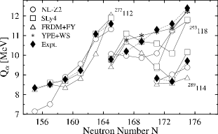
Figure 9: Comparison of experimental and calculated $Q_{\alpha}$ values for the decay chains of ${}^{277}_{165}112$, ${}^{289}_{175}114$, and ${}^{293}_{175}118$ (left panel) and the $\alpha$–decay chain leading through ${}^{292}_{176}$116 (right panel), in the latter three cases following the mass and charge assignment of the experimental groups. For odd-$N$ nuclei the calculated values from SLy4 and NL–Z2 connect the lowest states with positive parity in all cases, while the FRDM+FY and YPE+WS data are ground state to ground state values. Data taken from Ben00a ; dubna .

The experimental values follow a smooth trend while most mean-field results have a pronounced kink at $N=176$. This is a shell effect related to predicted deformed shells which is not reflected in the data. The resolution of that puzzle lies in correlation effects. The PES of these SHE are rather soft (see also the previous subsection). The ground state then explores large fluctuations in quadrupole deformation $\beta_{2}$ and the pure mean-field minimum is insufficient in such a situation. One has at least to evaluate the correlation effects for $\beta_{2}$ motion, for an example from stable nuclei see e.g. girod . Applying such a scheme to the chain of SHE indeed yields a smooth trend of the $Q_{\alpha}$ Rei00a , but this aspect of correlations goes beyond the scope of this paper.

IV Conclusions

We have reviewed self-consistent models for nuclear structure, thereby concentrating on the two most widely used brands: the relativistic mean-field model (RMF) and the non-relativistic Skyrme–Hartree–Fock model (SHF). A brief discussion of the formal properties has shown the relation between these two models and to nuclear bulk properties. Each term in the SHF energy can be directly connected with a bulk property (as e.g. volume energy, asymmetry energy, etc). An exception is, of course, the spin-orbit term which disappears in bulk matter. The RMF can be connected with SHF by virtue of a non-relativistic expansion in orders of $v/c$ and in orders of meson range. The basic structures are fully comparable whereas the details of density dependence differ. An advantage of the RMF is that the spin-orbit force is automatically included without the need of separate tuning. The SHF, on the other hand, is superior in its flexibility to accommodate isovector forces. Both models contain a good handful of free parameters which need to be adjusted phenomenologically. Different demands and bias in the adjustment has led to a world of different forces, in SHF as well as in RMF. We have selected an overseeable set of typical forces to display the possible variations in the results. The basic properties for normal nuclei are all very well reproduced by all chosen forces. An interesting detail is the isotope shift of radii in Pb. The remarked kink at the magic ²⁰⁸Pb is immediately reproduced by the RMF but can only be described within SHF after an appropriate extension of the (isovector) spin-orbit force.

The discussion of results has concentrated on superheavy elements (SHE). The average error of binding energies in known SHE covers a larger span than the error in stable nuclei. This is an expected result because extrapolations always tend to scatter the errors. The positive aspect is that all errors remain in bearable bounds (safely below 1 $\%$) and that there remain even several forces which maintain the quality found in stable nuclei. A different feature is given by looking at the relative errors of binding energies nucleus by nucleus, thus displaying the trends in these errors. The quality in reproducing the trends is found to be independent from the average quality of the binding energies. Large differences between the forces are seen for the trends in mass number $A$ and neutron excess $N-Z$ where the SHF forces generally perform better with respect to these trends. A different way to look at trends is provided by the two-nucleon separation energies and $Q_{\alpha}$ values. The $Q_{\alpha}$ for recently discovered chains of SHE are nicely reproduced within $\pm 1$ MeV for the more recent and well adjusted parametrisations in SHF and RMF. Somewhat more variance is found for the separation energies (not shown in this paper). The trend of the trends is given with the two-nucleon shell gaps, i.e. the difference of adjacent separation energies. They depend predominantly on shell structure (unlike binding and separation energies which are also influenced by the bulk properties of a force). Large gaps serve as an indicator for magic shell closures. The predictions on the two-nucleon shell gaps vary substantially, to the extend that different forces predict shell closures at different proton numbers. The differences look less dramatic if one realises that the overall size of the two-nucleon shell gaps is small in any case. The concept of magic shell closures seems to fade away in SHE. One has to remind that magic shells had been looked for as a simple guideline where to find SHE which are sufficiently shell-stabilised against Coulomb pressure towards spontaneous fission. The ultimate, but hard to evaluate, criterion is the height of the fission barrier. Simpler to compute is the shell-correction energy which can serve as a rough estimate: large negative shell-correction energy is a necessary condition for stability against fission. We find for all forces a broad valley of large shell correction energies. This a welcome feature as it leaves some freedom in the choice of the reaction channels. Thus we see good chances to hit many more SHE in near future experiments, in spite of the fact that pronounced doubly magic systems will not be found.

The investigations have demonstrated the high descriptive power of nowadays mean-field models. They have also revealed some weak points where further fine-tuning is needed, taking advantage of the many new data from exotic nuclei in general and SHE in particular. Last not least, one explores the limits of mean-field models when going towards the limits of stability. Shape coexistence and subsequent need for correlation effects shows up notoriously for the less well bound nuclei.

Acknowledgements

We would like to thank our collaborators T. Bürvenich, S. Ćwiok, D. J. Dean, J. Dobaczewski, P. Fleischer, W. Greiner, A. Kruppa, W. Nazarewicz, Ch. Reiß, K. Rutz, T. Schilling, M. R. Strayer, and T. Vertse for their contributions and helpful hints. We also acknowledge many inspiring discussions with our experimental colleagues J. Friedrich, S. Hofmann G. Münzenberg, V. Ninov, and Yu. Ts. Oganessian. This work was supported by Bundesministerium für Bildung und Forschung (BMBF), Project No. 06 ER 808 and by Gesellschaft für Schwerionenforschung (GSI). The Joint Institute for Heavy Ion Research has as member institutions the University of Tennessee, Vanderbilt University, and the Oak Ridge National Laboratory; it is supported by the members and by the Department of Energy through Contract No. DE–FG05–87ER40361 with the University of Tennessee.

References

- (1) S. G. Nilsson, I. Ragnarsson, Shapes and Shells in Nuclear Structure, Cambridge University Press, 1995.
- (2) M. Brack, J. Damgård, A. S. Jensen, H. C. Pauli, V. M. Strutinsky, C. Y. Wong, Rev. Mod. Phys. 44, 320 (1972).
- (3) M. Brack, Proc. of the “International Workshop on Nuclear Structure Models”, Oak Ridge, Tennessee, March 16–25, 1992, edited by R. Bengtsson, J. Draayer, W. Nazarewicz, World Scientific, Singapore, 1992, page 165.
- (4) U. Mosel, W. Greiner, Z. Phys. 222, 261 (1969).
- (5) S. G. Nilsson, C. F. Tsang, A. Sobiczewski, Z. Szymanski, S. Wycech, C. Gustafson, I.–L. Lamm, P. Möller, B. Nilsson, Nucl. Phys. A131, 1 (1969).
- (6) Yu. A. Lazarev et al., Phys. Rev. C 54, 620 (1996).
- (7) S. Hofmann, Rep. Prog. Phys. 61, 639 (1998).
- (8) S. Hofmann, G. Münzenberg, Rev. Mod. Phys. 72, 733 (2000).
-
(9)
Yu. Ts. Oganessian et al.,
Nature 400, 242 (1999),
Yu. Ts. Oganessian et al., Phys. Rev. Lett. 83, 3154 (1999),
Yu. Ts. Oganessian et al., Phys. Rev. C 62, 041604 (2000). - (10) Yu. Ts Oganessian et al., Phys. Rev. C 63, 011301(R) (2001).
- (11) V. Ninov et al., Phys. Rev. Lett. 83, 1104 (1999).
- (12) P. Armbruster, Eur. Phys. J. A7, 23 (2000).
- (13) F. P. Hessberger et al., Z. Phys. A359, 415 (1997).
- (14) P. Reiter et al., Phys. Rev. Lett. 82, 509 (1999).
- (15) M. Leino et al., Eur. Phys. J. A6, 63 (1999).
- (16) J. Dechargé, D. Gogny, Phys. Rev. C 21, 1568 (1980).
- (17) J.–F. Berger, J. Dechargé, D. Gogny, Proc. of the “International Workshop on Nuclear Structure Models”, Oak Ridge, Tennessee, March 16–25, 1992, edited by R. Bengtsson, J. Draayer, W. Nazarewicz, World Scientific, Singapore, 1992.
-
(18)
S. A. Fayans, E. L. Trykov, D. Zawischa,
Nucl. Phys. A568, 523 (1994),
S. A. Fayans, S. V. Tolokonnikov, E. L. Trykov, D. Zawischa, Nucl. Phys. A676, 49 (2000). - (19) B. A. Nikolaus, T. Hoch, D. G. Madland, Phys. Rev. C 46, 1757 (1992).
- (20) W. H. Dickhoff, H. Müther, Rep. Prog. Phys. 11, 1947 (1992).
- (21) H. Heiselberg, V. Pandharipande, Annu. Rev. Nucl. Part. Sci. 50, 481 (2000).
-
(22)
J. W. Negele, D. Vautherin,
Phys. Rev. C 5, 1472 (1972),
J. W. Negele, D. Vautherin, Phys. Rev. C 11, 1031 (1975). - (23) W. D. Myers, Droplet Model of Atomic Nuclei, IFI/Plenum, New York, 1977.
- (24) P. Möller, J. R. Nix, W. D. Myers, W. J. Swiatecki, Atom. Nucl. Data Tables 59, 185 (1995).
-
(25)
P. Möller, J. R. Nix,
Nucl. Phys. A549, 84, (1992),
P. Möller, J. R. Nix, J. Phys. G 20, 1681, (1994). - (26) E. K. U. Gross, R. M. Dreizler, Density functional theory, Springer, Berlin 1990.
- (27) I. Zh. Petkov, M. V. Stoitsov, Nuclear Density Functional Theory, Clarendon Press, Oxford, 1991.
- (28) J. Dobaczewski, J. Dudek, Proc. of “High Angular Momentum Phenomena, Workshop in honour of Zdzisław Szymański”, Piaski, Poland, August 23–26, 1995, Acta Physica Polonica B27, 45 (1996).
- (29) P.–G. Reinhard, C. Toepffer, Int. J. Mod. Phys. E3, 435 (1994).
- (30) Y. Aboussir, J. M. Pearson, A. K. Dutta, F. Tondeur, Nucl. Phys. A549, 155 (1992).
-
(31)
W. D. Myers, W. J. Swiatecki,
Phys. Rev. C 58, 3368 (1998),
W. D. Myers, W. J. Swiatecki, Phys. Rev. C 60, 54313 (2000). -
(32)
D. Vautherin, D. M. Brink,
Phys. Rev. C 5, 626 (1972),
M. Beiner, H. Flocard, N. Van Giai, P. Quentin, Nucl. Phys. A238, 29 (1975). -
(33)
T. H. R. Skyrme,
Phil. Mag. 1, 1043 (1956),
T. H. R. Skyrme, Nucl. Phys. 9, 615 (1959). -
(34)
J. S. Bell, T. H. R. Skyrme,
Phil. Mag. 1, 1055 (1956),
T. H. R. Skyrme, Nucl. Phys. 9, 635 (1959). - (35) M. Jaminon, C. Mahaux, Phys. Rev. C40, 354 (1989), and references therein.
-
(36)
O. Haxel, J. H. D. Jensen, H. E. Suess,
Phys. Rev. 75, 1766 (1949),
M. Göppert–Mayer, Phys. Rev. 75, 1969 (1949),
M. Göppert–Mayer, Phys. Rev. 78, 16 (1950),
M. Göppert–Mayer, Phys. Rev. 78, 22 (1950). - (37) P. Ring, P. Schuck, The nuclear many-body problem, Springer (1980).
- (38) E. Chabanat, P. Bonche, P. Haensel, J. Meyer, R. Schaeffer, Nucl. Phys. A635, 231 (1998), Nucl. Phys. A643, 441(E) (1998).
-
(39)
M. Brack, P. Quentin,
Phys. Lett. 56B, 421 (1975),
M. Brack, C. Guet, H.–B. Håkansson, Phys. Rep. 123, 275 (1985). - (40) P.–G. Reinhard, H. Flocard, Nucl. Phys. A584, 467 (1995).
- (41) P.-G. Reinhard, Ann. Phys. (Leipzig) 1, 632 (1992).
- (42) H.–P. Duerr, Phys. Rev. 103, 469 (1955).
- (43) B. D. Serot, J. D. Walecka, Phys. Lett. 87B, 172 (1979).
- (44) J. Boguta, A. R. Bodmer, Nucl. Phys. A292, 413 (1977).
-
(45)
R. N. Schmid, E. Engel, R. M. Dreizler,
Phys. Rev. C 52, 164 (1995),
R. N. Schmid, E. Engel, R. M. Dreizler, Phys. Rev. C 52, 2804 (1995). - (46) P.–G. Reinhard, Rep. Prog. Phys. 52, 439 (1989).
- (47) B. D. Serot, Rep. Prog. Phys. 55, 1855 (1992).
- (48) P. Ring, Prog. Part. Nucl. Phys. 37, 193 (1996).
- (49) P.–G. Reinhard, Z. Phys. A329, 257 (1988).
- (50) Y. Sugahara, H. Toki, Nucl. Phys. A579, 557 (1994).
- (51) M. Thies, Phys. Lett. B166, 23 (1986)
- (52) M. Bender, K. Rutz, P.–G. Reinhard, J. A. Maruhn, Eur. Phys. J. A8, 59 (2000).
- (53) M. Bender, K. Rutz, P.–G. Reinhard, J. A. Maruhn, Eur. Phys. J. A7, 467 (2000).
- (54) F. Tondeur, S. Goriely, J. M. Pearson, M. Onsi, Phys. Rev. C 62, 024308 (2000).
- (55) J. Friedrich, P.–G. Reinhard, Phys. Rev. C 33, 335 (1986).
- (56) J. Bartel, P. Quentin, M. Brack, C. Guet, H.–B. Håkansson, Nucl. Phys. A386, 79 (1982).
- (57) J. Dobaczewski, H. Flocard, J. Treiner, Nucl. Phys. A422, 103 (1984).
- (58) F. Tondeur, M. Brack, M. Farine, J. M. Pearson, Nucl. Phys. A420, 297 (1984).
- (59) M. Rufa, P.–G. Reinhard, J. A. Maruhn, W. Greiner, M. R. Strayer, Phys. Rev. C 38, 390 (1989).
- (60) G. A. Lalazissis, J. König, P. Ring, Phys. Rev. C 55, 540 (1997).
- (61) J. Friedrich, N. Voegler, Nucl. Phys. A373, 191 (1982).
- (62) M. M. Sharma, G. A. Lalazissis, J. König, P. Ring, Phys. Rev. Lett. 74, 3744 (1995).
- (63) J. P. Blaizot, J.–F. Berger, J. Dechargé, M. Girod, Nucl. Phys. A535, 331 (1995).
- (64) P.–G. Reinhard, Nucl. Phys. A649, 305c (1999).
-
(65)
T. Bürvenich, K. Rutz, M. Bender, P.–G. Reinhard, J. A. Maruhn,
W. Greiner,
Eur. Phys. J. A3, 139 (1998). - (66) M. Bender, Proc. of the International Conference on “Fusion dynamics at the extremes”, Dubna, Russia, May 25–27, 2000 (in print).
-
(67)
K. Rutz,
Doctoral Dissertation,
J. W. Goethe Universität Frankfurt am Main,
ibidem–Verlag Stuttgart, 1999. - (68) M. Bender, K. Rutz, P.–G. Reinhard, J. A. Maruhn, W. Greiner, Phys. Rev. C 60, 034304 (1999).
-
(69)
K. Rutz, M. Bender, T. Bürvenich, T. Schilling, P.–G. Reinhard,
J. A. Maruhn,
W. Greiner, Phys. Rev. C 56, 238 (1997). - (70) A. T. Kruppa, M. Bender, W. Nazarewicz, P.–G. Reinhard, T. Vertse, S. Ćwiok, Phys. Rev. C 61, 034313 (2000).
- (71) P.–G. Reinhard, M. Bender, W. Nazarewicz, unpublished results.
- (72) K. Rutz, M. Bender, P.–G. Reinhard, J. A. Maruhn, W. Greiner, Nucl. Phys. A634, 67 (1998).
- (73) R. R. Kinsey et al., The NUDAT/PCNUDAT program for nuclear data, 9th International Symposium of Capture Gamma-Ray Spectroscopy and Related Topics (Budapest, Hungary), October 1996, Data extracted from the NUDAT database, version March 20, 1997, National Nuclear Data Center, Brookhaven National Laboratory.
- (74) M. Sanchez–Vega et al., Phys. Rev. C 60, 024303 (1999).
- (75) J. Dechargé, J.-F. Berger, K. Dietrich, M. S. Weiss, Phys. Lett. B451, 275 (1999).
- (76) P.–G. Reinhard , J. Friedrich, N. Voegeler, Z. Phys. A316, 207 (1984).
-
(77)
M. Bender, K. Rutz, P.–G. Reinhard, J. A. Maruhn, W. Greiner,
Phys. Rev. C 58, 2126 (1998). -
(78)
S. Ćwiok, J. Dobaczewski, P.–H. Heenen, P. Magierski, and
W. Nazarewicz,
Nucl. Phys. A611, 211 (1996). -
(79)
P.–G. Reinhard, D. J. Dean, W. Nazarewicz, J. Dobaczewski, J. A. Maruhn,
and
M. R. Strayer, Phys. Rev. C 60, 14316 (1999). - (80) A. N. Andreyev, et al., Nature 405, 430 (2000).
- (81) J.–F. Berger, L. Bitaud, J. Dechargé, M. Girod, and S. Peru-Dessenfants, Proc. of the “International Workshop XXXIV on Gross Properties of Nuclei and Nuclear Exitations”, Hirschegg, Austria, 1996, edited by H. Feldmeier, J. Knoll, and W. Nörenberg (GSI, Darmstadt, 1996), p. 56.
- (82) S. Ćwiok, P.–H. Heenen, W. Nazarewicz, Phys. Rev. Lett. 83, 1108 (1999).
- (83) M. Bender, Phys. Rev. C 61, 031302(R) (2000).
- (84) S. Ćwiok , S. Hofmann, W. Nazarewicz, Nucl. Phys. A573, 356 (1994).
- (85) M. Girod, P.–G. Reinhard, Nucl. Phys. A384, 179 (1982).
- (86) P.–G. Reinhard, M. Bender, T. Bürvenich, T. Cornelius, P. Fleischer, J. A. Maruhn, Proc. of the “Tours Symposium on Nuclear Physics IV”, Tours, France, September 2000 AIP, in print.