The Two-Time Green’s Function and Screened Self–Energy for Two-Electron Quasi-Degenerate States

Abstract

Precise predictions of atomic energy levels require the use of QED, especially in highly-charged ions, where the inner electrons have relativistic velocities. We present an overview of the two-time Green’s function method; this method allows one to calculate level shifts in two-electron highly-charged ions by including in principle all QED effects, for any set of states (degenerate, quasi-degenerate or isolated). We present an evaluation of the contribution of the screened self-energy to a finite-sized effective hamiltonian that yields the energy levels through diagonalization.

1 Experiments and Theory

Experimental measurements of atomic energy levels provide more and more stringent tests of theoretical models; thus, the experimental accuracy of many measurements is better than the precision of theoretical calculations: in hydrogen 51debeauvoir97 ; 51huber99 , in helium 51dorrer97 ; 51drake96 , and in lithium-like uranium 51schweppe91 and bismuth 51beiersdorfer98 . The current status of many precision tests of Quantum-Electrodynamics in hydrogen and helium can be found in this edition.

Furthermore, highly-charged ions possess electrons that move with a velocity which is close to the speed of light. The theoretical study of such systems must therefore take into account relativity; moreover, a perturbative treatment of the binding to the nucleus (with coupling constant $Z\alpha$) fails in this situation 51yerokhin00 . Perturbative expansions in $Z\alpha$, however, are useful in different situations (see 51pachucki98b for a review, and articles in this edition 51karshenboim2000 ; 51melnikov2000 ; 51andreev2000 ; 51ivanov2000 ).

2 Theoretical Methods for Highly-Charged Ions

There are only a few number of methods that can be used in order to predict energy levels for highly-charged ions within the framework of Bound-State Quantum Electrodynamics 51mohr89 : the adiabatic $S$-matrix formalism of Gell-Mann, Low and Sucher 51sucher57 , the evolution operator method 51vasilev75 ; 51zapryagaev85 , the two-time Green’s function method 51shabaev94 and an interesting method recently proposed by Lindgren (based on Relativistic Many-Body Perturbation Theory merged with QED) 51lindgren00 . All these methods are based on a study of the some evolution operator or propagator; the two extreme times of the propagation can be both infinite (Gell-Mann–Low–Sucher), one can be finite and the other infinite (Lindgren), and both can be finite (Shabaev).

But among these methods, only two can in principle be used in order to apply perturbation theory to quasi-degenerate levels (e.g., the ³P₁ and ¹P₁ levels in helium-like ions): the two-time Green’s function method and Lindgren’s method (which is still under development). Both work by constructing a finite-sized effective hamiltonian whose eigenvalues give the energy levels 51shabaev93 .

The two-time Green’s function method has the advantage of being applicable to many atomic physics problems, such as the recombination of an electron with an ion 51shabaev94b , the shape of spectral lines 51shabaev91 and the effect of nuclear recoil on atomic energy levels 51shabaev98 ; 51shabaev2000b .

2.1 Overview of the Two-Time Green’s Function Method

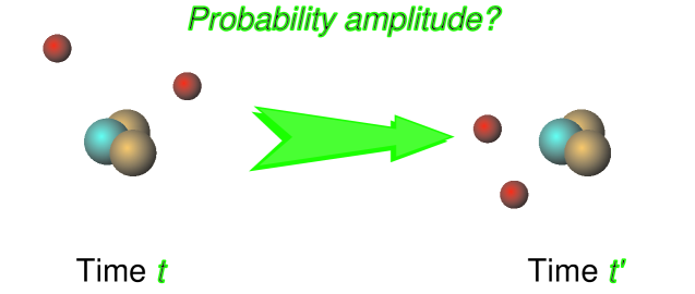
We give in this section a short outline of the two-time Green’s function method. The basic object of this method 51shabaev90 represents the probability amplitude for $N$ fermions to go from one position to the other, as shown in Fig. 1.

Figure 1: The 2-particle Green’s function is the amplitude for going from one state of two particles to another state

The corresponding mathematical object is a usual $N$-particle correlation function between two times:

$${S_{\mbox{\scriptsize{F}}}^{N}}^{\alpha_{1}\ldots\alpha_{N}}_{\alpha_{1}^{\prime}\ldots\alpha_{N}^{\prime}}({\mathbf{x}}_{1},\ldots,{\mathbf{x}}_{N},t;{\mathbf{x}}^{\prime}_{1},\ldots,{\mathbf{x}}^{\prime}_{N},t^{\prime})$$ (2)

$$\equiv \langle\Omega|\mbox{T}\,\hat{\Psi}^{\alpha_{1}}({\mathbf{x}}_{1},t)\cdots\hat{\Psi}^{\alpha_{N}}({\mathbf{x}}_{N},t)$$

$$\qquad\,\times\hat{\overline{\Psi}}_{\alpha_{N}^{\prime}}({\mathbf{x}}^{\prime}_{N},t^{\prime})\cdots\hat{\overline{\Psi}}_{\alpha_{1}^{\prime}}({\mathbf{x}}^{\prime}_{1},t^{\prime})|\Omega\rangle\,,$$

where $|\Omega\rangle$ is the vacuum of the full Bound-State QED Hamiltonian $\hat{H}$, and where the quantum field $\hat{\Psi}$ is defined as the usual canonical electron–positron field evolving under the total hamiltonian in the Heisenberg picture 51mohr89 .

A remark can be made here about Lorentz invariance: the above correlation function (or propagator) displays only two times, which are associated to many different positions. A Lorentz transform of the space–time positions involved therefore yields many different individual times (one for each position); thus, the object (2) must be defined in a specific reference frame. And this reference frame is chosen as nothing more than the Galilean reference frame associated to the nucleus, which is physically privileged.

Fundamental Property of the Green’s Function

The $N$-particle Green’s function is a function of energy simply defined through a Fourier transform of Eq. (2):

$${\mathcal{G}}^{N}({\mathbf{x}}_{1},\ldots,{\mathbf{x}}_{N};{\mathbf{x}}^{\prime}_{1},\ldots,{\mathbf{x}}^{\prime}_{N};E\in{\mathbb{R}})$$

$$\equiv \frac{1}{i}\int\!d\Delta t\,e^{iE\Delta t}\,S_{\mbox{\scriptsize{F}}}^{N}({\mathbf{x}}_{1},\ldots,{\mathbf{x}}_{N},\Delta t;{\mathbf{x}}^{\prime}_{1},\ldots,{\mathbf{x}}^{\prime}_{N},t^{\prime}=0)\,.$$ (3)

This function is interesting because it contains the energy levels predicted by Bound-State QED: one can show 51shabaev90 that

$${\mathcal{G}}^{N}({\mathbf{x}}_{1},\ldots,{\mathbf{x}}_{N};{\mathbf{x}}^{\prime}_{1},\ldots,{\mathbf{x}}^{\prime}_{N};E\in{\mathbb{R}})$$

$$= \sum_{\mbox{\scriptsize{\parbox{77.00017pt}{\centering Eigenstates $|n\rangle$ of $\hat{H}$ with charge~{}$-N|e|$\@add@centering}}}}\frac{\langle\Omega|{\hat{\psi}({\mathbf{x}}_{1})\cdots\hat{\psi}({\mathbf{x}}_{N})|n\rangle\langle n|\hat{\overline{\psi}}({\mathbf{x}}^{\prime}_{N})\cdots\hat{\overline{\psi}}({\mathbf{x}}^{\prime}_{1})}|\Omega\rangle}{E-(E_{n}-i0)}$$

$${}+(-1)^{N^{2}+1} \sum_{\mbox{\scriptsize{\parbox{77.00017pt}{\centering Eigenstates $|n\rangle$ of $\hat{H}$ with charge~{}$+N|e|$\@add@centering}}}}\frac{\langle\Omega|{\hat{\overline{\psi}}({\mathbf{x}}^{\prime}_{N})\cdots\hat{\overline{\psi}}({\mathbf{x}}^{\prime}_{1})|n\rangle\langle n|\hat{\psi}({\mathbf{x}}_{1})\cdots\hat{\psi}({\mathbf{x}}_{N})}|\Omega\rangle}{E-(-E_{n}+i0)}\,,$$

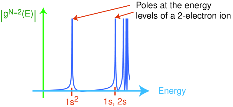
where $|\Omega\rangle$ is the vacuum of the total hamiltonian $\hat{H}$; $\hat{\psi}$ is the usual second-quantized Dirac field in the Schrödinger representation and $E_{n}$ is the energy of the eigenstate $n$ of $\hat{H}$. The poles in $E$ with a positive real part are exactly the energies of the states with charge $-N|e|$, which are physically the atomic eigenstates of an ion with $N$ orbiting electrons (The charge of the nucleus is not counted in the total charge.), as shown graphically in Fig. 2. Such a result is similar to the so-called Källén–Lehmann representation 51peskin95 .

Figure 2: The 2-particle Green’s function contains information about the atomic energy levels of a 2-electron atom or ion

In order to obtain the energy levels contained in (2), we must resort on a perturbative calculation of the correlation function (2), which belongs to standard textbook knowledge 51itzykson . The position of the poles of (2) must then be mathematically found. It is possible to construct an effective, finite-size hamiltonian which acts on the atomic state that one is interested in; the eigenvalues of this hamiltonian then give the Bound-State QED evaluation of the energy levels 51shabaev93 . This hamiltonian is obtained through contour integrations.

2.2 Second-Order Calculations

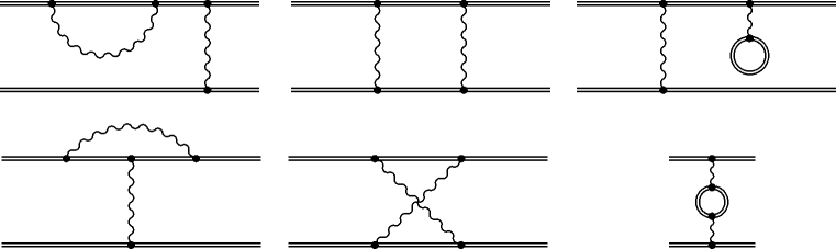
The current state-of-the-art in non-perturbative calculations (in $Z\alpha$) of atomic energy levels within Bound-State QED consists in the theoretical evaluation of the contribution of diagrams with two photons (i.e. of order $\alpha^{2}$, since the electron–photon coupling constant is $e$). For instance, for ions with two electrons, the screening of one electron by the other is described by the six diagrams of Fig. 3.

Figure 3: The contributions of order $\alpha^{2}$ to the electron-electron interaction

However, most of the calculations of contributions of order $\alpha^{2}$ were, until very recently, restricted to the very specific case of the ground-state (see 51yerokhin99 for references). The extension to the calculation of the energy levels of quasi-degenerate states represents one of the current trends of the research in the domain of non-perturbative (in $Z\alpha$) calculations with QED.

We have calculated the contribution of the screened self-energy (first and fourth diagrams of Fig. 3) to some isolated levels in 51yerokhin99 ; 51indelicato98a ; 51indelicato91 ; 51yerokhin99b . When energy levels are quasi-degenerate (e.g., the ³P₁ and ¹P₁ levels in helium-like ions), the two-time Green’s function method allows one to evaluate the matrix elements of the effective hamiltonian between different states; for the first diagram of Fig. 3, we obtain the following contribution to this hamiltonian (The two electrons on the left are denoted by $n_{1}$ and $n_{2}$, and the two on the right by $n^{\prime}_{1}$ and $n^{\prime}_{2}$, and other notations follow.):

$$\sum_{P,P^{\prime}}(-1)^{PP^{\prime}}\Bigg{\{}-\Big{(}\sum_{k\neq n^{\prime}_{P^{\prime}(1)}}\mbox{$\langle n_{P(1)}n_{P(2)}|$}S_{k}^{\mathrm{r}}(\varepsilon_{n_{P(1)}},\varepsilon_{n^{\prime}_{P^{\prime}(1)}})\mbox{$|n^{\prime}_{P^{\prime}(1)}n^{\prime}_{P^{\prime}(2)}\rangle$}$$

$$\qquad+\sum_{k\neq n_{P(1)}}\mbox{$\langle n_{P(1)}n_{P(2)}|$}S_{k}^{\mathrm{l}}(\varepsilon_{n_{P(1)}},\varepsilon_{n^{\prime}_{P^{\prime}(1)}})\mbox{$|n^{\prime}_{P^{\prime}(1)}n^{\prime}_{P^{\prime}(2)}\rangle$}\Big{)}$$ (5)

$$\quad+\frac{1}{2}\bigg{[}\left.\partial_{p}\right|_{\varepsilon_{n_{P(1)}}}\Big{(}\mbox{$\langle n_{P(1)}|$}\Sigma(p)\mbox{$|n_{P(1)}\rangle$}$$

$$\quad\qquad\times\mbox{$\langle n_{P(1)}n_{P(2)}|$}I(p-\varepsilon_{n^{\prime}_{P^{\prime}(1)}})\mbox{$|n^{\prime}_{P^{\prime}(1)}n^{\prime}_{P^{\prime}(2)}\rangle$}\Big{)}$$

$$\qquad+\left.\partial_{p^{\prime}}\right|_{\varepsilon_{n^{\prime}_{P^{\prime}(1)}}}\Big{(}\mbox{$\langle n_{P(1)}n_{P(2)}|$}I(\varepsilon_{n_{P(1)}}-p^{\prime})\mbox{$|n^{\prime}_{P^{\prime}(1)}n^{\prime}_{P^{\prime}(2)}\rangle$}$$

$$\quad\qquad\times\mbox{$\langle n^{\prime}_{P^{\prime}(1)}|$}\Sigma(p^{\prime})\mbox{$|n^{\prime}_{P^{\prime}(1)}\rangle$}\Big{)}\bigg{]}\Bigg{\}}$$

$$+\mathcal{O}[\alpha^{2}(E_{n^{\prime}}^{(0)}-E_{n}^{(0)})]\,,$$

where we made use of standard notations 51yerokhin99 : $\varepsilon_{k}$ is the energy of the Dirac state $k$, $(-1)^{PP^{\prime}}$ is the signature of the permutation $P\circ P^{\prime}$ of the indices $\{1,2\}$, $\Sigma$ represents the self-energy, and $I$ represents the photon-exchange:

$$\mbox{$\langle ab|$}I(\omega)\mbox{$|cd\rangle$} \equiv e^{2}\int\!d^{3}\vec{x}_{2}\,[\psi_{a}^{\dagger}(\vec{x}_{1})\alpha^{\mu}\psi_{c}(\vec{x}_{1})]$$

$$\times[\psi_{b}^{\dagger}(\vec{x}_{2})\alpha^{\nu}\psi_{d}(\vec{x}_{2})]D_{\mu\nu}(\omega;\vec{x}_{1}-\vec{x}_{2})$$

$$\mbox{$\langle a|$}\Sigma(p)\mbox{$|b\rangle$} \equiv \frac{1}{2\pi i}\int\!d\omega\,\sum_{k}\frac{\mbox{$\langle ak|$}I(\omega)\mbox{$|kb\rangle$}}{\varepsilon_{k}(1-i0)-(p-\omega)},$$ (7)

where $a,b,c$ and $d$ label Dirac states, and $e$ is the charge of the electron; $\alpha^{\mu}$ are the Dirac matrices, and $\psi$ denotes a Dirac spinor; the photon propagator $D$ is given in the Feynman gauge by:

$$D_{\nu\nu^{\prime}}(\omega;\vec{r})\equiv g_{\nu\nu^{\prime}}\frac{\exp\left(i|\vec{r}|\sqrt{\omega^{2}-\mu^{2}+i0}\right)}{4\pi|\vec{r}|},$$ (8)

where $\mu$ is a small photon mass that eventually tends to zero, and where the square root branch is chosen such as to yield a decreasing exponential for large real-valued energies $\omega$. In Eq. (5), $\partial_{x}\left|{}_{x_{0}}\right.$ is the partial derivative with respect to $x$ at the point $x_{0}$, and the skeletons of the screened self-energy diagrams with a self-energy on the left and on the right are defined as:

$$\mbox{$\langle n_{P(1)}n_{P(2)}|$}S_{k}^{\mathrm{r}}(p,p^{\prime})\mbox{$|n^{\prime}_{P(1)}n^{\prime}_{P(2)}\rangle$}\equiv$$

$$\qquad\mbox{$\langle n_{P(1)}n_{P(2)}|$}I(p-p^{\prime})\mbox{$|kn^{\prime}_{P^{\prime}(2)}\rangle$}\frac{1}{\varepsilon_{k}(1-i0)-p^{\prime}}\mbox{$\langle k|$}\Sigma(p^{\prime})\mbox{$|n^{\prime}_{P^{\prime}(1)}\rangle$}\,,$$

$$\mbox{$\langle n_{P(1)}n_{P(2)}|$}S_{k}^{\mathrm{r}}(p,p^{\prime})\mbox{$|n^{\prime}_{P(1)}n^{\prime}_{P(2)}\rangle$}\equiv$$

$$\qquad\mbox{$\langle n_{P(1)}|$}\Sigma(p)\mbox{$|k\rangle$}\frac{1}{\varepsilon_{k}(1-i0)-p}\mbox{$\langle kn_{P(2)}|$}I(p-p^{\prime})\mbox{$|n^{\prime}_{P(1)}n^{\prime}_{P(2)}\rangle$}\,.$$

The terms of order $\alpha^{2}(E_{n^{\prime}}^{(0)}-E_{n}^{(0)})$ are not included in the above expression because they do not contribute to the level shift of order $\alpha^{2}$ in which we are interested. (They contribute to higher orders, as can be seen in the particular case of two levels (51shabaev00, , p. 27).)

This expression is only formal and must be renormalized 51yerokhin99 ; angular integrations can then be done and numerical computations can be performed in order to yield the Bound-State QED evaluation of the energy shifts.

For the contribution of the first diagram of Fig. 3 to have any physical meaning, it is necessary to calculate it together with the vertex correction (fourth diagram of Fig. 3). We have obtained the following contribution to the effective hamiltonian for the vertex correction:

$$\sum_{P,P^{\prime}}(-1)^{PP^{\prime}}\sum_{i_{1},i_{2}}\mbox{$\langle i_{1}n_{P(2)}|$}I(\varepsilon_{n_{P(1)}}-\varepsilon_{n^{\prime}_{P^{\prime}(1)}})\mbox{$|i_{2}n^{\prime}_{P^{\prime}(2)}\rangle$}$$

$$\quad\times\frac{i}{2\pi}\int\!d\omega\,\frac{\mbox{$\langle n_{P(1)}i_{2}|$}I(\omega)\mbox{$|i_{1}n^{\prime}_{P^{\prime}(1)}\rangle$}}{[\varepsilon_{i_{1}}(1-i0)-(\varepsilon_{n_{P(1)}}-\omega)][\varepsilon_{i_{2}}(1-i0)-(\varepsilon_{n^{\prime}_{P^{\prime}(1)}}-\omega)]}$$

$$+\mathcal{O}[\alpha^{2}(E_{n^{\prime}}^{(0)}-E_{n}^{(0)})]$$

where $(n_{1},n_{2})$ and $(n^{\prime}_{1},n^{\prime}_{2})$ still represent the electrons of the two states that define the hamiltonian matrix element given here, and where the sum over $i_{1}$ and $i_{2}$ is over all Dirac states.

3 Conclusion and Outlook

We have presented a quick overview of the current status of theoretical predictions of energy levels in highly-charged ions with Bound-State Quantum Electrodynamics. We have given a short description of the two-time Green’s function method, which permits the calculation of an effective hamiltonian that can in principle include all QED effects in energy shifts. We have also presented the specific contribution of the screened self-energy in the general case (isolated levels, quasi-degenerate or degenerate levels); the expression obtained can serve as a basis for numerical calculations of the corresponding effective hamiltonian.

References

- (1) B. de Beauvoir, F. Nez, L. Julien, B. Cagnac, F. Biraben, D. Touahri, L. Hilico, O. Acef, A. Clairon, J. J. Zondy: Phys. Rev. Lett. 78, 440–443 (1997)
- (2) A. Huber, B. Gross, M. Weitz, T. W. Hänsch: Phys. Rev. A 59, 1844–1851 (1999)
- (3) C. Dorrer, F. Nez, B. de Beauvoir, L. Julien, F. Biraben: Phys. Rev. Lett. 78, 3658–3661 (1997)
- (4) G. W. F. Drake: ‘High precision calculation for Helium’. In: Atomic, Molecular and Optical Physics Handbook, ed. by G. W. F. Drake (AIP Press, Woodbury, New York 1996) pp. 154–171
- (5) J. Schweppe, A. Belkacem, L. Blumenfeld, N. Claytor, B. Feynberg, H. Gould, V. Kostroun, L. Levy, S. Misawa, R. Mowat, M. Prior: Phys. Rev. Lett. 66, 1434–1437 (1991)
- (6) P. Beiersdorfer, A. L. Osterheld, J. H. Scofield, J. R. C. López-Urrutia, K. Widmann: Phys. Rev. Lett. 80, 3022–3025 (1998)
- (7) V. A. Yerokhin: Phys. Rev. A 62, 012508 (2000)
- (8) K. Pachucki: Hyp. Inter. 114, 55–70 (1998)
- (9) S. G. Karshenboim: this edition pp. LABEL:c_kars–LABEL:c_kars_
- (10) K. Melnikov, T. van Ritbergen: this edition pp. LABEL:c_meln–LABEL:c_meln_
- (11) O. Andreev, L. Labzowsky: this edition pp. LABEL:c_andr–LABEL:c_andr_
- (12) V. G. Ivanov, S. G. Karshenboim: this edition pp. LABEL:c_ivan–LABEL:c_ivan_
- (13) P. J. Mohr: ‘Quantum electrodynamics of high- few-electron atoms’. In: Physics of Highly-ionized Atoms, ed. by R. Marrus (Plenum, New York 1989) pp. 111–141
- (14) J. Sucher: Phys. Rev. 107, 1448–1449 (1957)
- (15) A. N. Vasil’ev, A. L. Kitanin: Theor. Math. Phys. 24, 786–793 (1975)
- (16) S. A. Zapryagaev, N. L. Manakov, V. G. Pal’chikov: Theory of One- and Two-Electron Multicharged Ions (Energoatomizdat, Moscow 1985) in Russian
- (17) V. M. Shabaev, I. G. Fokeeva: Phys. Rev. A 49, 4489–4501 (1994)
- (18) I. Lindgren: Mol. Phys. 98, 1159–1174 (2000)
- (19) V. M. Shabaev: J. Phys. B 26, 4703–4718 (1993)
- (20) V. M. Shabaev: Phys. Rev. A 50, 4521–4534 (1994)
- (21) V. M. Shabaev: J. Phys. A 24, 5665–5674 (1991)
- (22) V. M. Shabaev: Phys. Rev. A 57, 59 (1998)
- (23) V. M. Shabaev: this edition pp. LABEL:c_shab–LABEL:c_shab_
- (24) V. M. Shabaev: Sov. Phys. J. 33, 660–670 (1990)
- (25) M. E. Peskin, D. V. Schroeder: An introduction to quantum field theory (Addison-Wesley, Reading, Massachusetts 1995)
- (26) C. Itzykson, J.-B. Zuber: Quantum Field Theory (McGraw-Hill 1980)
- (27) V. A. Yerokhin, A. N. Artemiev, T. Beier, G. Plunien, V. M. Shabaev, G. Soff: Phys. Rev. A 60, 3522–3540 (1999)
- (28) P. Indelicato, P. J. Mohr: Hyp. Int. 114, 147–153 (1998)
- (29) P. Indelicato, P. J. Mohr: Theor. Chem. Acta. 80, 207–214 (1991)
- (30) V. A. Yerokhin, A. N. Artemyev, T. Beier, V. M. Shabaev, G. Soff: Phys. Scr. T80, 495–497 (1999)
- (31) V. M. Shabaev: E-print physics/0009018 (September 2000) Submitted to Phys. Rep.