Entropy Production at High Energy and $\mu_{B}$

Abstract:

The systematics of bulk entropy production in experimental data on A+A, $p+p$ and $e^{+}e^{-}$ interactions at high energies and large $\mu_{B}$ is discussed. It is proposed that scenarios with very early thermalization, such as Landau’s hydrodynamical model, capture several essential features of the experimental results. It is also pointed out that the dynamics of systems which reach the hydrodynamic regime give similar multiplicities and angular distributions as those calculated in weak-coupling approximations (e.g. pQCD) over a wide range of beam energies. Finally, it is shown that the dynamics of baryon stopping are relevant to the physics of total entropy production, explaining why A+A and $e^{+}e^{-}$ multiplicities are different at low beam energies.

1 Introduction

Figure 1: Brunelleschi’s Duomo in Florence, seen from the outside (left) and inside (right). Externally, it is a simple, elegant structure, while complex internal “dynamics” are seen on the inside.

Brunelleschi’s dome was built in Florence in the 15th century and continues to impress due to its sheer size and technical achievements. And yet, examining it from the outside, you would never guess at the complex internal “dynamics” of Vasari and Zuccari’s interior frescoes, depicting choirs of angels, saints, and various sins. The point of this work is to argue something similar about our understanding of heavy ion collisions. Graphical displays of RHIC events look quite complicated, with thousands of tracks emanating from the primary vertex composed of a variety of particles. However, angular distributions of inclusive charged particles can be found to show simple “scaling” features, which are shared even with elementary collisions. Of course, just like the exterior structure provides the support for the frescoes inside, these scaling patterns may well hint at the true microscopic dynamics at work. In any case, scaling relations may well suggest an overall framework into which predictions relevant to the upcoming Large Hadron Collider (LHC) at CERN and FAIR at GSI should fit.

2 Elementary Collisions

Compared to RHIC collisions, “elementary” collisions of protons and antiprotons, or electrons and positrons, which produce many hadrons seem to look quite sparse. Thus, they are generally thought to result from very different physics processes.

Electron-positron annihilation into hadrons used to be understood using concepts based on the original “string models” of the 1970’s, with extensions incorporating multiple gluon production[1]. More recently, purely perturbative calculations involving gluon ladders can capture many features of the data, down to details of jet fragmentation. This is especially true of calculations of the total multiplicity, which have good descriptive and predictive power, starting from the early SPEAR data up to the top LEP2 energies. A full accounting of the running coupling in jet fragmentation gives formulae that scale as $n_{ch}\propto\alpha^{A}_{s}\exp(B\sqrt{\ln(s)})$[2]. One achieves similar results in various “parton cascade” approaches, such as JETSET, which augments the older string models with perturbative gluon emission.

Collisions of protons and antiprotons are generally understood in a “two-component” scenario. The soft component is thought to be the domain of “non perturbative QCD” but understood phenomenologically by means of descriptive features like longitudinal phase-space and limited $p_{T}$. Various implementations of this can be tuned to describe the available data. Of course, jet phenomena have been observed as the energies increased, suggesting that there is a separate “hard” component at work in p+p collisions. This has been successfully modeled by combining the structure functions measured at high-$Q^{2}$ in $e+p$ collisions, with pQCD cross sections to get the angular distributions, and fragmentation functions measured in $e^{+}e^{-}$ reactions used to parametrize the relationships between the outgoing quarks and gluons and the measured hadrons.

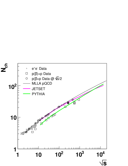
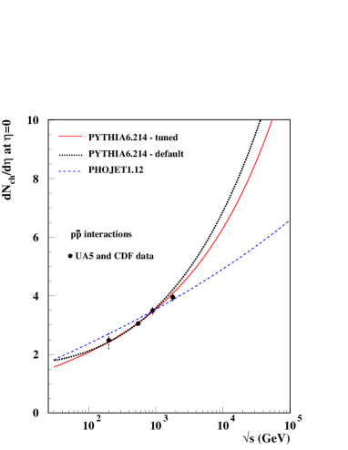
Figure 2: (left) Total primary charged particle multiplicity for $e^{+}e^{-}$ (with up to 10% admixture of weak decays) and $p(\overline{p})+p$ collisions, compared with MLLA pQCD calculations, JETSET, and PYTHIA. (right) Midrapidity density for $\overline{p}+p$ collisions vs. $\sqrt{s}$ compared with PYTHIA and PHOJET, from Ref. [7]

Various models incorporate the hard and soft components in different schemes, such as PYTHIA[3], HERWIG[4], PHOJET [5], and HIJING[6]. And yet, despite being based on similar inputs, most of these models predict different extrapolations of existing data to high energies [7], as shown in Fig. 2. One expects an interesting early running of the LHC while the various models (or tunings thereof) are validated, or ruled out, by the first data.

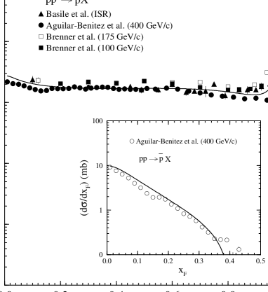
Figure 3: Inclusive $dN/dx_{F}$ for protons $p+p$ collisions at several energies. Inset shows the same for anti-protons. From Ref. [11].

One major uncertainty in understanding soft particle production in p+p (and $\overline{p}+p$) collisions is related to the lack of dynamical mechanisms in the models. It is still not generally understood how the incoming baryons are “stopped”, and their energy transmuted into particles[8]. The net rapidity loss of the incoming baryons has been studied extensively in fixed-target experiments as well as at the ISR (but not at the Tevatron collider, unfortunately) [9, 10]. It has been found that the distribution of $x_{F}=2p_{Z}/\sqrt{s}$, the fraction of energy found in the outgoing “leading” particles is essentially flat (but with a quasi-elastic peak near $x_{F}\sim 1$)[11], as shown in Fig. 3. More interestingly, this net baryon rapidity loss is found to correlate strongly with the total multiplicity, and approach the $e^{+}e^{-}$ multiplicity measured at the same $\sqrt{s}$[9]. In fact, the $e^{+}e^{-}$ and $p+p$ data overlap each other if $p+p$ is plotted at $\sqrt{s_{eff}}=\sqrt{s}/2$. This suggests that 1) the net baryons measured in p+p collisions reflect the inelasticity of the collision, and 2) the basic mechanisms of total entropy production in both $e^{+}e^{-}$ and $p+p$ are quite similar.

One way to understand the similarity between the entropy produced in these two systems is by simply postulating that both are the result of an equilibration process. Cooper, Frye and collaborators [12] worked under this assumption in the 1970’s. Thus, whatever complicated dynamics might be different between the two systems is rendered irrelevant by strong interactions between the fundamental constituent degrees of freedom. In that scenario, the rest of the evolution is isentropic and simply expresses the total entropy via the total multiplicity. Clearly, this is a difficult scenario to consider if one conceives of it proceeding via the kinetic equilibrium of the outgoing particles. However, it seems less problematic if the particles are thought to be the consequence of the freezeout of a fluid with many strongly-interacting degrees of freedom into the thousands of available mass states of QCD. This is the model that Fermi [13] and Landau [14] inadvertently proposed in the 1950’s.

3 Landau’s Hydrodynamical Model

Fermi and Landau both arrived at a simple formula for the total multiplicity in the early 1950’s[13, 14]. The derivation simply assumes complete thermalization of the total energy $E=\sqrt{s}$ in a Lorentz-contracted volume $V=V_{0}/\gamma=V_{0}/(\sqrt{s}/2m_{N})$, leading to an initial energy density $\epsilon=s/2m_{N}V_{0}$, which increases quadratically with $\sqrt{s}$. Assuming the blackbody equation of state $p=\epsilon/3$ and the first law of thermodynamics $d\epsilon=Td\sigma$, leads to a scaling of the entropy density as $\sigma\propto s^{3/4}$. Multiplying the entropy density by the volume gives a total entropy $S=\sigma V\propto s^{3/4}/s^{1/2}\propto s^{1/4}$. This is the famous Landau-Fermi multiplicity scaling formula, which suggests that total multiplicities will scale as the square root of the CMS energy, $N\propto\sqrt{E_{cm}}$. For a more generic equation of state (e.g. $\epsilon=c^{2}_{s}p$), $N\propto(1/2)(1-c^{2}_{s})/(1+c^{2}_{s})$ [12].

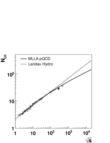
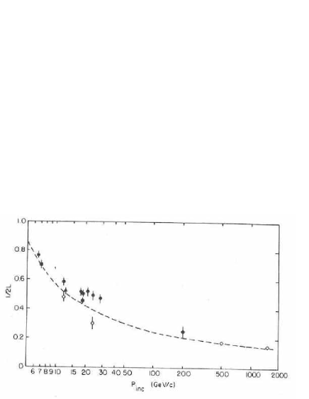
Figure 4: (left) $N_{ch}$ for $e^{+}e^{-}$ and $p(\overline{p})+p$ at $\sqrt{s_{eff}}=\sqrt{s}/2$ compared with MLLA pQCD and Landau Hydrodynamics. Both functions have been adjusted by an overall scale factor. (right) Fits to $1/2L$ for $p+p$ data over a range of energies, from Carruthers and Duong-Van [18].

While the pQCD formula mentioned above, shown in Fig.4, does a good job for the $e^{+}e^{-}$ data, the Landau-Fermi formula does an equally good job describing the high-energy data when tuned on the lower energy data. It also naturally explains the constant ratio between the $p+p$ and $e^{+}e^{-}$ data at the same $\sqrt{s}$, since $s^{1/4}_{eff}=\sqrt{1/2}\sim 70\%$. Of course, it remains an open question how higher-energy data will turn out, given that the two formulae differ significantly at much higher energies (pQCD giving $N_{ch}\sim 100$ and Landau giving $N_{ch}\sim 160$ at LHC energies) and the $\overline{p}+p$ data already seems to trend below even the pQCD prediction shown above.

Of course, the dynamical evolution does not end with the initial equilibrated system postulated by the Landau-Fermi model. Landau correctly recognized that if such a system achieves local equilibrium (i.e. with vanishingly-small mean free paths), it will behave hydrodynamically [14, 15]. The blackbody EOS implies a locally-traceless stress energy tensor, and thus scale-free (i.e. conformal) dynamics. Thus, the evolution of the system is determined only by the scales imposed at the beginning (the energy and volume) and at the end (the familiar freezeout condition such that evolution stops at $T=T_{ch}$)

Landau’s well-known initial conditions are quite simple: an enormous energy density with no longitudinal motion, packed into a volume contracted along the z axis by $1/\sqrt{s}$. Following the evolution analytically from its initial 1+1D expansion to the late 3+1D expansion (using various approximations along the way), he found that the rapidity distribution of the fluid elements at freezeout is described by a Gaussian distribution with variance $\sigma^{2}_{y}=(1/2)\ln(s/4m^{2}_{N})\equiv L$. Cooper, Frye and Schonberg completed the modern interpretation of hydrodynamics by suggesting that the fluid elements are not particles but hadronic fireballs which decay isotropically in their own rest frame[12]. Carruthers and Duong Van found that Landau’s model was a better fit to data than the boost-invariant scenarios popular at the time [18], as shown in Fig.4.

It is worth taking a few moments to remark on what the Landau model is: It is a 3+1D model which assumes rapid local equilibration and has no free parameters. It has two scales, $\sqrt{s}$ and $T_{ch}$ which determine the initial and final states. Finally, it describes the energy dependence of the produced entropy and its angular distributions. There is no nuclear transparency in the model and no assumption of boost-invariance. Rather, the entire system is explicitly assumed to be in local thermal contact on asymptotically small time scales $t_{0}~{}1/\sqrt{s}$ as the beam energy increases.

And a few words on what the Landau model is not: There is no description of net-baryon dynamics (or those of any conserved charges). There is no phase transition, but just a single EOS $p=\epsilon/3$. There is no hadronization per se, but just a simple freezeout criterion ($T=T_{ch}$), and thus no mass dependence of $dN/dy$ (something which was discussed in the 1970’s by Cooper and Frye) and certainly no resonance decays. Since these are clearly important pieces of physics, clearly seen in data, these issues should be seen as caveats for the various conclusions drawn later.

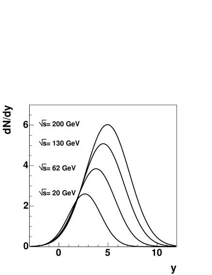
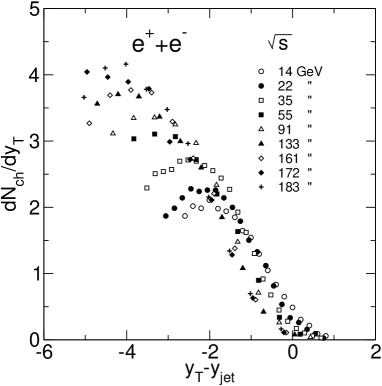
Figure 5: (left) Calculations of $dN/dy$ (with an arbitrary overall scale) the Landau hydrodynamic model (Equation 3.1), seen in the fixed target frame, showing “extended longitudinal scaling”. (right) $dN/dy_{T}$, the rapidity distribution along the thrust axis in $e^{+}e^{-}$ collisions, viewed in the frame of the outgoing quark ($y_{T}-y_{jet}$), from Ref.[20].

One very non-trivial feature of Landau’s hydrodynamical model appears when it is combined with the Landau-Fermi multiplicity formula

$$\frac{dN}{dy}=Ks^{1/4}\frac{1}{\sqrt{2\pi L}}\exp\left(-\frac{y^{2}}{2L}\right)$$ (1)

and then viewed in the rest frame of one of the projectiles by making the transformation $y^{\prime}=y-y_{beam}=y-(L+\ln(2))$, where $L=\ln(\sqrt{s}/2m_{P})$

$$\frac{dN}{dy^{\prime}}\sim\frac{1}{\sqrt{L}}\exp\left(-\frac{y^{\prime 2}}{2L}-y^{\prime}\right)$$ (2)

One sees that this is approximately a function of $y^{\prime}$ alone, especially near $y^{\prime}=0$, with some slight scale breaking. A direct plot of $dN/dy^{\prime}$ at several beam energies, shown in the left panel of Fig. 5, shows the phenomenon of “limiting fragmentation” or “extended longitudinal scaling” [17] even more clearly. While not an original observation about the Landau model (see e.g. Ref.[18]), this scaling was rediscovered in this context in Ref.[19]. This is a non trivial outcome of the formulae, and is even more intriguing considering that it is clearly seen in both $p+p$ and $\overline{p}+p$ data with respect to the beam axis, as well as $e^{+}e^{-}$ data with respect to the thrust axis [20] as shown in the right panel of Fig. 5.

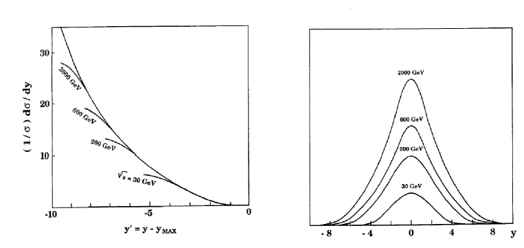
Figure 6: MLLA pQCD calculations, from Ref.[21], showing rapidity distributions in the rest frame of the outgoing quark (left) and in the CM frame (right).

But the surprises of Landau’s model are not just limited to its relevance to experimental data. The calculations of jet fragmentation in perturbative QCD, in the MLLA framework discussed above, have been done by several authors during the 1980’s. In Ref.[21], Tesima performed MLLA pQCD calculations (which have a different anomalous dimension than Mueller’s, and thus presumably a different energy dependence) for the rapidity distribution of emitted gluons. He found that the rapidity was approximately gaussian with a width scaling as $\sqrt{\ln(s)}$ and “translational invariance”, seen by observing the fragmentation functions as a function of $y^{\prime}=y-y_{max}$. Finally, we have already seen that the MLLA formula gives similar multiplicities to the Landau-Fermi formula over energy ranges for which data exist. Thus, we find that, even parametrically, pQCD and the Landau model can give similar results. Whether this is a particularly ornate accident, or whether the mathematics (non-Abelian gauge theories, and 3+1D hydrodynamics with Landau’s initial conditions and freezeout criterion) share a deep underlying structure seems to be a particularly intriguing question.

The prevalence of extended longitudinal scaling in elementary collisions, and the predictions of this phenomenon from both MLLA pQCD and Landau’s hydrodynamical model should not be forgotten when discussing the phenomenon in A+A in the context of newer theoretical frameworks, some of which will be discussed in the next section. The theoretical predictions for this scaling should also be kept in mind when trying to predict the shape of $dN/d\eta$ and the value of $dN/d\eta(\eta=0)$, e.g. in Ref.[22]. While the data suggests a “linear” trend to the limiting curve, the models shown here (both pQCD and Landau) suggest a nonlinearity as the energy increases, as seen in Figs.5 and 6.

4 Heavy Ion Collisions

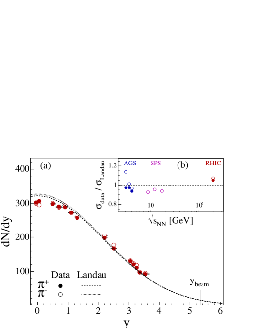
Figure 7: Rapidity distribution of pions measured in A+A by BRAHMS. The inset shows the comparisons of Gaussian fits over a wide range of $\sqrt{s_{NN}}$ divided by the Landau prediction $\sigma_{Landau}=\log(\sqrt{s}/2m_{P})$.

Moving from elementary collisions to heavy ion collisions brings in a large number of new dynamical considerations. The initial state should be characterized by shadowed parton distribution functions, as well as the nuclear geometry suggested by Glauber calculations. The early dynamics are driven by hard parton scattering and subsequent reinteractions, possibly leading to equilibration. Eventually the momentum transfers become low enough that hadron formation is preferred, and the quark chemistry freezes out, incorporating the thermalized quarks as well as the ones from jet fragmentation. These hadrons themselves may rescatter if the densities are sufficiently high, leading to an eventual thermal freeze-out. Finally, the final-state hadrons themselves decay, either immediately via strong processes, or over macroscopic distances via weak processes. All of these stages are in principle independent of the others, and thus could lead to a non-trivial energy and geometrical dependence as the relative contributions of soft and hard processes change (e.g. HIJING [6]) as well as rescattering in the partonic and/or hadronic phases [23].

Surprisingly, the simple behavior in particle multiplicities seen in $p+p$ and $e^{+}e^{-}$ collisions are quite similar to what is actually found in A+A collisions. The rapidity distributions of pions measured by BRAHMS [24] and experiments at lower energies appear to be Gaussian, as seen in Fig. 7, and approximately follow the Landau predictions from 1955. The angular distributions at RHIC also clearly show extensive longitudinal scaling [25], as shown in Fig. 8. More interestingly, the limiting curve is wider in more peripheral events, with a long tail extending to large $\eta$ (which may be partially explained by the presence of spectators with substantial $p_{T}$, but not completely). Combining this fact with the decreasing multiplicity near mid-rapidity in more peripheral events, it is found that the overall multiplicity (subtracting part of the tail using phenomenological fits to extend into the unmeasured region) is approximately constant when dividing out by the number of participant pairs ($N_{part}/2$). This is shown in Fig. 8 for a wide range of energies measured at RHIC [25, 26].

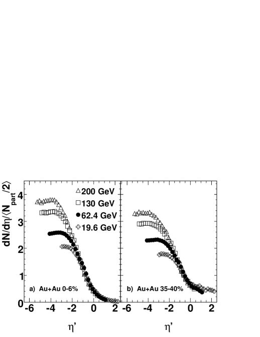
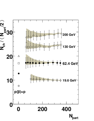
Figure 8: (left) Extended longitudinal scaling for Au+Au collisions at RHIC, from Ref.[25]. (right) Total multiplicity divided by the estimated number of participant pairs, as a function of $N_{part}$, from Ref.[25].

The absence of a strong centrality dependence makes it possible to compare $N_{ch}/(N_{part}/2)$ in A+A with other systems [26]. As discussed above, the $p+p$ data is similar to the $e^{+}e^{-}$ if one takes the $\sqrt{s}$ to be an effective $\sqrt{s_{eff}}=\sqrt{s}/2$, accounting for the average $x_{F}$ of the leading particles. This is assuming that the flat $dN/dx_{F}$ distribution is mainly comprised of baryons that do not participate in the thermalization or subsequent dynamical evolution. Conversely, it is found that A+A and $e^{+}e^{-}$ data are similar to one another between $\sqrt{s}=20-200$ GeV without any other adjustments except dividing by $N_{part}/2$ [26], as shown in Fig.9. Given the previous comparisons of $p+p$ and $e^{+}e^{-}$, one particular efficient way to understand the comparisons with A+A is to postulate that the multiple collisions experienced by each participant (as $\nu>2-3$ for all centralities considered in Ref. [26]) essentially stops all of the incoming energy. This alleviates the leading particle effect, and thus one finds the multiplicity per participant pair to be “universal” without additional scaling.

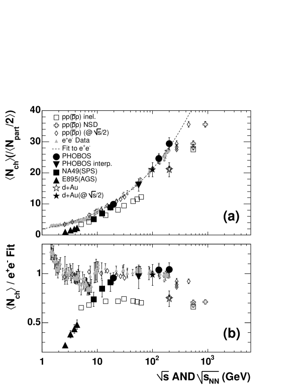
Figure 9: (top) Compilation of the total multiplicity for various systems, from Ref.[26]. (bottom) Data divided by the MLLA-based fit to the $e^{+}e^{-}$ data.

These comparisons are somewhat mysterious if one considers $e^{+}e^{-}$ reactions as involving just the physics of perturbative gluon radiation, while A+A is usually discussed in terms of a strongly-interacting partonic medium [27]. These two appear at first glance to be completely opposite limits of QCD physics, the very hard and very soft. However, it was mentioned above that parametrically, MLLA pQCD and Landau hydrodynamics are quantitatively very similar in their output, even if they do not appear to have similar functional forms. The Fermi-Landau scenario would also naturally predict that the multiplicity should scale linearly with the initial volume, which is clearly compatible with (and essentially predicted) the linear scaling of the total multiplicity with $N_{part}$ shown above. The same angular distributions as a function of $\sqrt{s}$ predicted by Landau also seem to appear in the elementary collisions as well. Perhaps it is not necessary to use heavy nuclei to achieve local equilibration. It should be kept in mind that only the first radiations in a hard process are at a truly hard scale. Subsequent gluon emissions require the summations of more-and-more complicated many-gluon diagrams, which perhaps drive the final distributions toward something resembling local equilibrium.

5 Some Predictions for the LHC

It seems natural here to try and make predictions for the LHC with the Landau model. From the basic formula, the midrapidity density scales as $\rho_{0}(\sqrt{s})\propto s^{1/4}/\sqrt{\ln\left(\sqrt{s}/2m_{P}\right)}$ – with no free parameters. Thus, the ratio of $\sqrt{s}=14$ TeV to $\sqrt{s}=200$ GeV in proton-proton collisions will be $\rho_{0}(14TeV)/\rho_{0}(200GeV)\sim 6.1$. The ratio of $\sqrt{s_{NN}}=5.5$ TeV to $\sqrt{s_{NN}}=200$ GeV for A+A (where $\rho_{0}$ is scaled by $N_{part}/2$) will be $\rho_{0}(5.5TeV)/\rho_{0}(200GeV)\sim 4.0$. This is shown in Fig.10, which includes $\rho_{0}$ for several types of collisions. Fits of the Landau energy dependence to data of each type (RHIC data for A+A, NSD UA5 data for $\overline{p}+p$) have been made, to account for the different $p_{T}$ distributions as well as the overall multiplicity scale.

It is interesting that while the formula gets the higher energy RHIC data (and section 5 will attempt and explanation for the lack of agreement at lower energies), the description of the $p+p$ and $\overline{p}+p$ is less satisfactory, even qualitatively. Unfortunately, there may be several factors which could lead to this. Considering yields at mid-rapidity makes comparisons more sensitive to the details of particle production, both species and $p_{T}$ dependence. There are also issues to do with triggering, especially the contribution from diffractive events, which are not well understood theoretically, and are difficult to control experimentally unless one is actively measuring leading particles. These factors would certainly complicate a trivial application of the Landau formula for $dN/dy$ in a limited region of $dN/d\eta$. Clearly, the LHC will be an interesting place to test these ideas over a large range of $\sqrt{s}$.

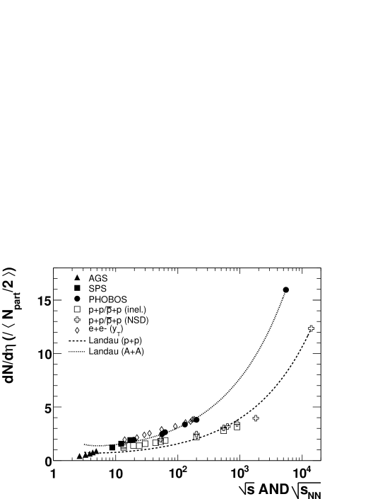
Figure 10: Midrapidity density for A+A, $p+p$ and $e^{+}e^{-}$ as a function of $\sqrt{s}$ and $\sqrt{s_{NN}}$. Calculations of the Landau predictions are superimposed, each fit to high energy A+A and $p+p$ data, with points showing the LHC predictions made in this work. The A+A calculations agree reasonably while the $p+p$ fit is less satisfactory over the full range.

6 Total Multiplicity at Finite $\mu_{B}$

And yet, it is clear that while all of the systems are similar between $20-200$ GeV, the heavy ion data is systematically below the $e^{+}e^{-}$ and $p+p$ data below 20 GeV, with progressively larger deviations with decreasing beam energies. This might suggest that the “universality” of bulk particle production described in Section 4 (and explained here by the surprising relevance of Landau’s hydrodynamical model) is broken at lower energies. However, a natural explanation of these data can be constructed by considering the role of the incoming baryons, an important dynamical issue ignored in Landau’s papers. The following discussion is based primarily on Ref.[28].

It was discussed above that the leading particles in $p+p$ collisions (generally thought to be the initial protons) take a fraction of the initial energy ($x_{F}=2p_{z}/\sqrt{s}$) with a distribution that is flat over most of $x_{F}$ (leading to $\langle x_{F}\rangle\sim 1/2$), suggesting that $dN/dy\sim exp(y)$. Contrary to this, measurements of the net-baryon ($p-\overline{p}$) $dN/dy$ in A+A collisions over a wide range of $\sqrt{s_{NN}}$ find that the net baryon density “piles up” at mid-rapidity at low energies and probably peaks at around $y\sim 4$ at RHIC energies [29]. The interplay between the net baryon density (which is conserved) and the rest of the particle production which is produced mainly by the freezeout of the strongly-interacting matter, requires a baryochemical potential in thermal fits to the yields of various hadron species [30]. This is shown in the right panel of Fig. 11 (from Ref. [28]) and is found to increase with decreasing beam energy, as the overall net baryon density increases.

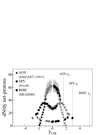
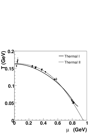
Figure 11: (left) Net baryon density for central A+A collisions at three CM energies, from Ref.[29]. (right) Compilation of extracted values of $T$ and $\mu_{B}$, as presented in Ref. [28]. Two parametrizations of $T(\mu_{B})$ are shown, as described in the text.

The depletion of the net-baryon density near mid-rapidity has been called “transparency” by several authors. This interpretation persists despite no corroborative evidence that the final distribution is simply from slowing down the initial-state baryons. Conversely, if one looks at the entropy alone, e.g. comparing A+A to $e^{+}e^{-}$ as was done in the previous section, one could arrive at the conclusion that the energy was fully stopped. It is possible that the initial baryons are carried along by the strong longitudinal expansion implied by Landau’s initial conditions (which is, ironically, much weaker than that described by Bjorken’s hydrodynamical model [31]). Thus, at the very least, one should consider the net baryon $dN/dy$ as the “net” rapidity distribution of the initial state baryon excess, after both dynamical stopping and re-acceleration stages.

As an example of a physical scenario which could generate the BRAHMS results, consider the formation of a “Fireball Sandwich”. It is based on the simple assumption that a single collision of a baryon on a target attenuates half of it’s energy (as seen in the comparison of the total entropy produced in $p+p$ reactions compared with $e^{+}e^{-}$) while practically all of the energy is dissipated in the next collision – a statement suggested, but not completely proved, by the flat centrality dependence of $N_{ch}/(2N_{part})$ in A+A collisions which is 40% higher than $p+p$ [26]. If this is the case, then while the first collision of each incoming baryons in each nucleus is not sufficient to stop it, the second (or perhaps third) might be. This will lead to both nuclei being fully stopped in the initial state of the collision (as needed for Landau’s hydrodynamic model to work) but each cluster of nucleons will be displaced from $z=0$ along the original direction of motion. It is not difficult to assume that the deposited energy will be mainly at $z=0$ and thus behind the two walls of baryons on the outside of the reaction zone. This creates a “sandwich” configuration, with layers of the incoming net baryons tending to be near the edges of the hot thermalized matter. These steps are illustrated (crudely) in Fig. 12.

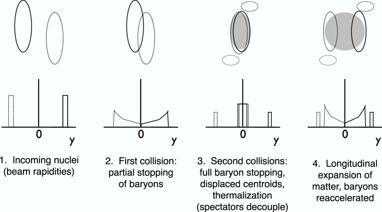
Figure 12: The “Fireball Sandwich” scenario for two colliding nuclei.

A key feature of hydrodynamic models is the strong correlation between the final state rapidity and the initial position of a fluid element relative to the light cone [15]. Fluid elements closer to the outside edge of the initial thermalized region will be pushed from behind and hadronize at large rapidities. Conversely, fluid elements near the center of the reaction zone will (unsurprisingly) hadronize near mid-rapidity. Thus, the Fireball Sandwich scenario naturally explains how a net-baryon $dN/dy$ resembling “transparency” could be generated from completely-stopped baryons. Of course, it does not explain the dynamical mechanisms behind baryon stopping, but it might allow experimental measurements to gain insight into the space-time structure of stopping in A+A collisions.

If the baryons are ultimately in the initial reaction, and the system is locally strongly-coupled, then it is almost inevitable that the will participate in the overall chemistry of the reaction, including the total entropy – and thus the total multiplicity. This can be seen by writing down the Gibbs potential for a system with a conserved baryon number:

$$G=E+PV-TS=\mu_{B}N_{B}$$ (3)

This rearranges to

$$S=\frac{E+PV}{T}-\frac{\mu_{B}N_{B}}{T}\equiv S_{0}-S_{B}.$$ (4)

This shows that the presence of a baryochemical potential reduces the total entropy, and thus the total multiplicity. If one scales out the total participating baryon number $N_{B}=N_{part}$ then the change in $N_{ch}/(N_{part}/2)$ is

$$\Delta N_{ch}\propto\frac{S_{B}}{N_{B}}\propto\frac{\mu_{B}}{T}$$ (5)

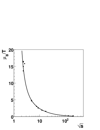
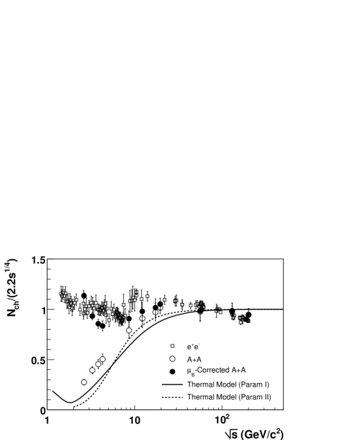
Figure 13: (left) $\mu_{B}/T$ vs. $\sqrt{s}$ extracted from data, as compiled in Ref.[28]. (right) Comparison of $e^{+}e^{-}$ and A+A data with two methods of estimating the effect of the net baryon density, 1) “correcting” the A+A data to approximate $\mu_{B}=0$ and 2) direct thermal model calculations using $\mu_{B}(\sqrt{s})$ and $T(\mu_{B}(\sqrt{s}))$ with two parametrizations.

Of course, applying this formula to real data requires a “baryon free” reference system for $N_{ch}$. It has been shown above that $p+p$ and $e^{+}e^{-}$ show the same energy dependence over a large range in $\sqrt{s}$, if one corrects for the leading particle effect. However, the presence of the leading baryons in the $p+p$ final state might make it a more complicated reference system, suggesting the use of $e^{+}e^{-}$ alone. But once this reference system is chosen, there are (at least) two strategies for understanding the role of baryon number on entropy production. One is to “correct” the A+A data for the presence of a non-zero $\mu_{B}$, with help from thermal model phenomenology. The other is to do a straightforward thermal model calculation to see how the entropy density is modified as a function of $T$ and $\mu_{B}$ and translate this into a “suppression” of $N_{ch}$ as a function of $\sqrt{s}$.

To correct the experimental data, it is only needed to calculate $\mu_{B}/T$ as a function of $\sqrt{s}$ and then find the constant of proportionality (assumed to be energy independent) to convert this to an inclusive charged-particle multiplicity. If $S/N=4$ and $N/N_{ch}=3/2$ (which is trivially true for a Boltzmann gas of massless pions), then the conversion factor between $S/N$ and $N_{ch}/(N_{part}/2)$ is exactly 6. Full thermal model calculations including strong decays give a comparable factor of 7.2, only 15% different than the trivial estimate. Thus, one adds $\Delta N_{ch}=(2./7.2)\mu_{B}/T$ to the measured value of $N_{ch}/(N_{part}/2)$ using the $\mu_{B}$ and $T$ extracted at each energy. For simplicity, we use a parametrization of $\mu_{B}(\sqrt{s})=1.2735/(1+0.2576\sqrt{s})$ extracted from the data shown in Fig. 11. To convert $\mu_{B}$ into $T$, we use two parametrizations of $T(\mu_{B})$, one assuming that $\langle E\rangle/\langle N\rangle=1GeV$ (“Thermal I”, adapted from Ref. [30]) and one using a third-order polynomial in $\mu^{2}_{B}$ (“Thermal II”).

The direct calculation method is based on the formula:

$$\frac{2}{N_{part}}\frac{N^{A+A}_{ch}}{N^{e^{+}e^{-}}_{ch}}=\frac{C^{A+A}}{C^{e^{+}e^{-}}}\frac{V^{A+A}}{V^{e^{+}e^{-}}}\frac{s(T,\mu_{B})}{s_{0}}$$ (6)

where the formulae above are used to convert $\sqrt{s}$ to $T$ and $\mu_{B}$, and it is assumed that $C^{A+A}=C^{e^{+}e^{-}}$ and $V^{A+A}=V^{e^{+}e^{-}}$. While assuming an equivalent conversion from entropy to multiplicity seems natural, equating the hadronization volume in $e^{+}e^{-}$ and the volume per participant pair in A+A seems less so. It may well be a corollary result of this work that it is not necessary to assume otherwise. In any case, this calculation predicts the entropy suppression as a function of $\sqrt{s}$ just based on experimental fits to ratios of particle yields. Thus, it has no free parameters and provides an approach complementary to the correction method.

The final results for both the correction method and the direct thermal model calculation are shown in Fig.13. The difference between them is a reasonable estimate for the systematic uncertainties on these phenomenological approaches. It is observed that the corrected A+A data more or less falls in line with the $e^{+}e^{-}$ data, and that the direct thermal model calculations (a purely theoretical calculation) qualitatively describe the suppression of the total multiplicity in A+A relative to $e^{+}e^{-}$ (a ratio based purely on experimental data). While the agreement is certainly not perfect, no attempts have been made to improve it by introducing ad hoc correction factors.

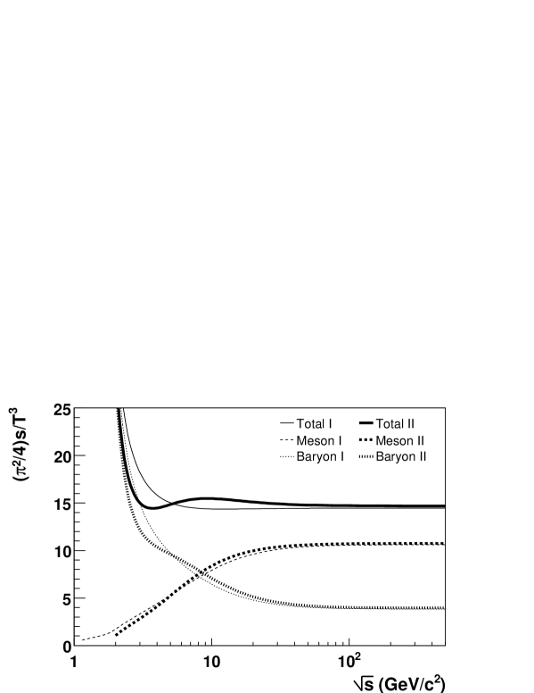
Figure 14: The entropy density divided by $T^{3}$ as a function of $\sqrt{s}$ for mesons only, baryons only, and the total. Again,two parametrizations are shown. The scaling by $(4/\pi^{2})$ transforms $s/T^{3}$ into the number of degrees of freedom of a massless relativistic Boltzmann gas.

It should be pointed out that all of the results shown in this work are for inclusive charged hadrons. This tends to be by necessity in the experiments represented here, which only measure inclusive charged particles. However, there are theoretical reasons for including all particles, and not choosing only mesons, as is often done in the literature. Fig. 14 shows a plot from Ref. [32] performed for the two parametrizations, but which is based on a figure shown in Ref. It shows that the entropy per $T^{3}$, which is equal to the number of degrees of freedom in a massless relativistic Boltzmann gas when multiplied by $\pi^{2}/4$, is constant above $\sqrt{s}=3GeV$ if one considers contributions from both baryons and mesons. It is manifestly not constant with $\sqrt{s}$ if one chooses one or the others. In particular, the meson sector rises very quickly and then plateaus, something seen in the NA49 “kink” plot [33].

7 Summary and Outlook

By showing how the low energy $A+A$ data can be made compatible with $e^{+}e^{-}$ data simply by considering the net baryon density, this completes, in principle, the “unification” of the systematics of charged particle production in high energy multiparticle reactions. From the comparisons of data shown above, one can glean three “rules of thumb” to understand the difference between the various systems.

• The effective energy has a direct relationship to the entropy (observed in $e^{+}e^{-}$ vs. $p+p$ and then in comparison to A+A)

• A stopped net baryon density suppresses the total entropy (observed in $e^{+}e^{-}$ vs. $A+A$ at low energies)

• These connections are only seen when one uses $N_{ch}$, i.e. one does not choose a particular measure of entropy.

It has been proposed here that the concepts and even the calculations of Landau’s hydrodynamic model can explain the relevance of these rules. Using rapid equilibration and hydrodynamic evolution as guiding concepts to describe the “bulk” physics in A+A as well as $e^{+}e^{-}$ and $p+p$ seems to have qualitative and quantitative value, and some new predictions for LHC energies have been given here. Arguing that $e^{+}e^{-}$ already has a comprehensive theory may lead to missing insights to be gained from asking why apparently different theories give similar results (e.g. why some pQCD calculations agree parametrically with Landau hydro).

Whatever the theoretical situation, detailed measurements of similar observables at higher energies or at high $\mu_{B}$ should provide crucial new information. The LHC will provide $p+p$ and A+A simultaneously, and FAIR at GSI will be specifically devoted to systems with large net baryon stopping and thus high $\mu_{B}$. In the high $\sqrt{s}$ sector, one will be testing the abilities of the system to thermalize, or not, on astoundingly short timescales of $O(10^{-}3fm/c)$. In the high $\mu_{B}$ sector one may be able to explore the systematics of baryon stopping to understand the mechanisms of energy deposition. Ultimately, one would like to understand all of this physics in relation to the microscopic processes suggested by QCD. In the meantime, the elegant structure of the data itself may well point theory in completely new directions or suggest unexpected connections between various techniques.

References

- [1] T. Sjostrand, arXiv:hep-ph/9508391.
- [2] A. H. Mueller, Nucl. Phys. B 228, 351 (1983).
- [3] T. Sjostrand, S. Mrenna and P. Skands, JHEP 0605, 026 (2006).
- [4] G. Marchesini, B. R. Webber, G. Abbiendi, I. G. Knowles, M. H. Seymour and L. Stanco, Comput. Phys. Commun. 67, 465 (1992).
- [5] R. Engel, Z. Phys. C 66, 203 (1995).
- [6] M. Gyulassy and X. N. Wang, Comput. Phys. Commun. 83, 307 (1994).
- [7] A. Moraes, C. Buttar and I. Dawson. SN-ATL-2006-057, CERN Document (ATLAS Scientific Note - Public) August 2006. To be published in The European Physics Jounal Direct.
- [8] W. Busza and A. S. Goldhaber, Phys. Lett. B 139, 235 (1984).
- [9] M. Basile et al., Phys. Lett. B 92, 367 (1980).
- [10] A. E. Brenner et al., Phys. Rev. D 26, 1497 (1982).
- [11] M. Batista and R. J. M. Covolan, Phys. Rev. D 59, 054006 (1999).
- [12] F. Cooper, G. Frye and E. Schonberg, Phys. Rev. Lett. 32, 862 (1974).
- [13] E. Fermi, Prog. Theor. Phys. 5, 570 (1950).
- [14] L. D. Landau, Izv. Akad. Nauk Ser. Fiz. 17, 51 (1953).
- [15] S. Z. Belenkij and L. D. Landau, Nuovo Cim. Suppl. 3S10, 15 (1956) [Usp. Fiz. Nauk 56, 309 (1955)].
- [16] P. Carruthers, Annals N.Y.Acad.Sci. 229, 91 (1974).
- [17] B. B. Back et al., Phys. Rev. Lett. 91, 052303 (2003).
- [18] P. Carruthers and M. Doung-van, Phys. Rev. D 8, 859 (1973).
- [19] P. Steinberg, Acta Phys. Hung. A 24, 51 (2005).
- [20] B. B. Back et al., Nucl. Phys. A 757, 28 (2005).
- [21] K. Tesima, Z. Phys. C 47, 43 (1990).
- [22] W. Busza, Acta Phys. Polon. B 35, 2873 (2004).
- [23] Z. W. Lin, C. M. Ko, B. A. Li, B. Zhang and S. Pal, Phys. Rev. C 72, 064901 (2005).
- [24] I. G. Bearden et al., Phys. Rev. Lett. 94, 162301 (2005).
- [25] B. B. Back et al., Phys. Rev. C 74, 021901 (2006).
- [26] B. B. Back et al., Phys. Rev. C 74, 021902 (2006).
- [27] M. Gyulassy and L. McLerran, Nucl. Phys. A 750, 30 (2005).
- [28] J. Cleymans, M. Stankiewicz, P. Steinberg and S. Wheaton, arXiv:nucl-th/0506027
- [29] I. G. Bearden et al., Phys. Rev. Lett. 93, 102301 (2004).
- [30] J. Cleymans and K. Redlich, Phys. Rev. Lett. 81, 5284 (1998).
- [31] J. D. Bjorken, Phys. Rev. D 27, 140 (1983).
- [32] J. Cleymans, H. Oeschler, K. Redlich and S. Wheaton, arXiv:hep-ph/0607164.
- [33] S. V. Afanasiev et al., Phys. Rev. C 66, 054902 (2002).