Hotter, Denser, Faster, Smaller…and Nearly-Perfect: What’s the matter at RHIC?

Abstract

The experimental and theoretical status of the “near perfect fluid” at RHIC is discussed. While the hydrodynamic paradigm for understanding collisions at RHIC is well-established, there remain many important open questions to address in order to understand its relevance and scope. It is also a crucial issue to understand how the early equilibration is achieved, requiring insight into the active degrees of freedom at early times.

1 Introduction

In April 2005, the four experiments at RHIC made a joint announcment of the discovery of a “perfect liquid” in high energy Au+Au collisions [1, Arsene:2004fa, 2, 3, 4]. This discovery has made quite an impression in the popular press, resulting in articles in Scientific American (April 2006) and Discover magazine (February 2007). It even was called the most important scientific story of 2005 by the American Institute of Physics [5]. While the press release was somewhat short on details, it offered a tantalizing glimpse of the connections with subjects as far afield as black holes and string theory, suggesting that they offered possible insight into the strongly-coupled system formed at RHIC.

The foundation of these discoveries was the success of ideal hydrodynamics in modeling the experimental data in a robust way. In other words, the system formed at RHIC turns out to be best seen as a single system that evolves collectively, rather than an ensemble of individual nucleon-nucleon collisions. The goal of this review is to outline the techniques and successes to date of hydrodynamics at RHIC, discuss the possible experimental and theoretical limits of this interpretation, and show how the current data points to new horizons in both regimes.

2 The “Perfect Fluid” at RHIC

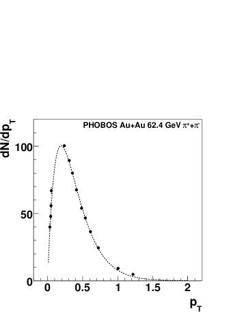
Figure 1: PHOBOS $dN/dp_{T}$ for charged pions at $\sqrt{s_{NN}}=62.4$ GeV. A Boltzmann fit is shown.

In hydrodynamical calculations for RHIC physics, there are typically three basic stages [6, 7]: initial conditions, hydrodynamic evolution, and freeze-out. The initial conditions consist of defining the energy density in position space, with each fluid cell given an initial velocity (note that these are purely classical calculations!). The aspects most interesting for RHIC collisions are when the spatial distribution of the initial energy density is highly anisotropic. This is because the second stage of the collision takes place while the system remains in local thermal equilibrium and evolves according to the evolution equations of hydrodynamics:

$$\partial_{\mu}T^{\mu\nu}=0$$ (1)

which are closed by the equation of state $p=f(\epsilon)$ e.g. $p=\epsilon/3$ for a gas of photons or QCD at high temperatures [8]. During this period, gradients in pressure and energy density induce an expansion and associated cooling of the system. As the local energy density decreases, so does the temperature ($T\propto\epsilon^{1/4}$). When a fluid element cools to the scale of the Compton wavelength of the pion $T_{ch}\sim m_{\pi}$, the system is considered to be sufficiently dilute that it decouples or “freezes-out” of the evolution and is transformed into hadrons. This occurs as an isotropic decay of the available energy density into known hadrons with thermal abundances in the fluid rest frame [9, 10].

While this physical scenario was invented in the early 1950’s and studied through the 1970’s, it was eventually discarded as a good model for strong interactions. Many rejected the possibility that small systems had sufficient time (or, strong enough coupling of the different fluid elements) to achieve any sort of local thermal or chemical equilibrium, much less a kinetic equilibirium of the final state particles, as suggested by Hagedorn in the 1960’s [11] based on the exponential rise of the hadron mass spectrum.Heavy ion collisions are larger and generate higher multiplicities, leading to a general expectation that equilibrium is likely.

In RHIC collisions, circumstantial hints of early-time thermalization shows up in the relative population of various hadron states, both as a function of particle mass and transverse momentum. The transverse momentum dependence, shown in Fig. 1 from Ref. [12] fit by a Boltzmann distribution, has the familiar form of the blackbody spectrum: $f(p,m)=1/(\exp[(\sqrt{p^{2}+m^{2}}-\mu_{B})/T]\pm 1)$ although it is obviously a “strong blackbody” with hadrons in the place of photons.

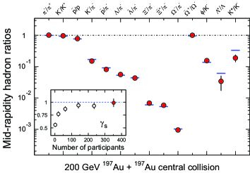
Figure 2: (left) STAR data on hadron ratios fit to a thermal model, from Ref. [4].

When the spectrum of each particle species is integrated $N(m)\propto V\int d^{3}pf(p,m)$, it is conventional to take ratios of particle yields to cancel out the common volume factor. This simple “thermal model” [13, 14] depends primarily on two parameters, the freeze-out $T_{ch}$ and the baryon chemical potential $\mu_{B}$ (defined such that $\overline{p}/p\sim exp(-2\mu_{B}/T_{ch})$). The experimental data on hadron yields is fit to a model incorporating these paramters (and all the known strong decays of high mass resonances to the observed particles) to estimate $T_{ch}$ and $\mu_{B}$. Typical values from recent fits are $T_{ch}=177$ MeV [4], corresponding to $2\times 10^{12}K$. According to the hydrodynamical scenario outlined above, this suggests that all possible hadron states are available to the system as it freezes out, so it may well make sense to assume that the relevant degrees of freedom active before the freezeout were also in thermal and chemical equilibrium. This itself implies that the system was substantially hotter than $T_{ch}$ for most of the evolution, especially at the very beginning. Thus, $10^{12}$ degrees is the coolest the system can be! It should be noted, however, that the relevance of a single temperature does not imply that the entire system freezes out in some sort of “global” equilibrium. Rather, this temperature seems to reflect the local properties of the system induced by the properties of the known hadron spectrum.

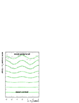
Figure 3: Charged $dN/d\phi$ relative to the event plane for for different centralities in $\sqrt{s_{NN}}=200$ GeV Au+Au collisions from PHOBOS.

If the system is in local equilibrium just before freezeout, then it is certainly plausible that it could show hydrodynamic behavior. Hydrodynamics implies the relevance of thermodynamics, but of course not the converse does not necessarily hold true [9]. At RHIC (and other machines colliding nuclei) it has been noticed that the event-by-event angular distribution is not isotropic in azimuthal angle. An “event plane” can be estimated from the produced particles, defined as angle $\Psi_{R}$ of the long principal axis of the particle angles. The azimuthal distribution relative to this event plane is found to show a strong $\cos(2[\phi-\Psi_{R}])$ dependence, shown in Fig. 3, from Ref. [15]. This is especially pronounced in more peripheral (i.e. lower multiplicity) collisions, where the overlap of the nuclei is shaped like an almond, relative to central (i.e. higher multiplicity) collisions where the overlap is essentially isotropic. This leads to a characterization of the event-by-event angular distributions in terms of its Fourier coefficients [17]:

$$\frac{dN}{d\phi}=1+2v_{1}\cos(\phi-\Psi_{R})+2v_{2}\cos(2[\phi-\Psi_{R}])+\cdots$$ (2)

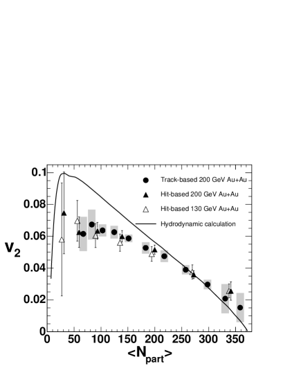
Figure 4: The elliptic flow parameter $v_{2}$ vs. $N_{part}$ for $\sqrt{s_{NN}}=200$ GeV from PHOBOS compared with a hydrodynamical model.

One of the early and striking results from RHIC was the measurement of $v_{2}$ – conventionally called “elliptic flow” – as a function of centrality (e.g. the number of participating nucleons $N_{part}$), an example of which is shown in Fig. 4 from Ref. [18]. The data show the qualitative features described above, that peripheral collisions have a large value of $v_{2}$, reflecting the large asymmetry in the initial distribution of nucleons, while the central collisions have a much smaller value. Hydrodynamic calculations use estimates of various properties (e.g. energy or entropy density) of the initial conditions by extrapolating from lower-energy data, and turn out to compare well to the data for $N_{part}>200$ [19]. At lower energies, similar calculations often overpredicted $v_{2}$ by factors of two, so RHIC data is considered striking validation of the hydrodynamic approach.

Comparing the relevant energy and space-time scales implied by the success of the hydrodynamical models, the matter at RHIC is formed under quite extreme conditions. The estimates of the formation time relevant for the hydrodynamic calculations were predicted to be in the vicinity of $\tau_{0}=0.6$ fm/c, or approximately 2 yoctoseconds ($10^{-24}$)[19]. This number is far smaller than the time taken a massless particle to traverse the radius of a hadron ($\tau\sim 1$ fm/c) [20]. At this time, the energy density needed to match the data is around $\epsilon=30$ GeV/fm³. This should be compared with the energy density of a nucleon in its rest frame, $\epsilon_{N}\sim 500$ MeV/fm³, which it exceeds by a factor of 60. And in the same sense as $T_{ch}$ is a lower limit of the system temperature at early times, these estimates do not preclude even higher energy densities at even earlier times. All of this depends on exactly when the system can be said to be in local thermal equilibrium, i.e. on the precise value of $\tau_{0}$.

Thus, to summarize, the success of the hydrodynamic models at RHIC suggest that collisions there make something that is hotter, denser, smaller, and faster (in the sense of thermalization time) than other known liquids. Furthermore, ideal hydrodynamics is inviscid by construction, i.e. there are no non-equilibrium processes encoded by the equations, at least until freezeout. In this light, the appelation of “perfect fluid” seems quite reasonable.

3 The Edge of Liquidity: The “Near Perfect Fluid”

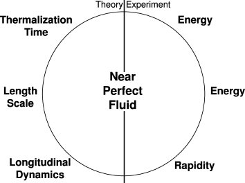
Figure 5: Frontiers of the hydrodynamic paradigm

However, it does not take much serious inquiry to raise a few doubts on this conclusion. No viscosity was needed to reproduce the data within experimental and theoretical uncertainties. And yet, it is not obvious that incorporating viscosity to some level would make the models completely disagree with the experimental data. Thus, it may be a “nearly” perfect liquid instead of a merely perfect liquid. But what exactly characterizes a “liquid”, as opposed to a strongly coupled gas? Both are fluids, while liquids are distinguished by attractive interactions between the constituents that generate a surface tension. Of course some sort of attractive interactions generate the bound-state hadrons in the final state, but this says nothing about earlier times.

Thus, until the precise form of the interaction can be shown to be uniformly attractive, and until it can be demonstrated that the system evinces no viscosity, the appellation “perfect liquid” should probably be replaced by the “near perfect fluid”. This does not reduce the importance of the RHIC discoveries. Rather it points to future investigations in both experiment and theory to elucidate the detailed microscopic properties of this system. In the meantime, we will assume the near-perfect fluid interpretation as a paradigm for looking at the RHIC data. The idea will be to vary certain parameters in experiment and theory, to see if any major changes take place that are qualitatively different from what is observed in the most-central collisions.

In order to probe the limits of this near-perfect fluid paradigm one can push to the “edge of liquidity” (shown schematically in Fig.5 experimentally (in energy, geometry, or rapidity) or theoretically (in thermalization time, length scale, or longitudinal dynamics) to see if the qualitative behavior changes. One way to examine the roles energy and geometry simultaneously, we can consider the systematics of elliptic flow simultaneously as a function of energy, centrality and system size. In the past 15 years, a large data set on $v_{2}$ has been measured near $\eta=0$ in the center-of-mass frame as a function of energy and centrality [2, 3, 4]. However, it is was only realized very recently that the data can be understood to depend on only several variables via the construction of “scaling relations” [23, 31]. These hold despite the enormous change in the available phase space as the energy increases, as evidenced by the higher multiplicities and the wider rapidity distributions.

Calculations performed with ideal hydrodynamics indicate that the magnitude of $v_{2}$ is mainly driven by the eccentricity of the initial-state matter distribution [21], where the eccentricity $\epsilon$ is defined as

$$\epsilon_{std}=\frac{\sigma^{2}_{Y}-\sigma^{2}_{X}}{\sigma^{2}_{Y}+\sigma^{2}_{X}}$$ (3)

where $\sigma^{2}_{X}$ is the variance in the direction along the reaction plane and $\sigma^{2}_{Y}$ is the variance perpendicular to it.

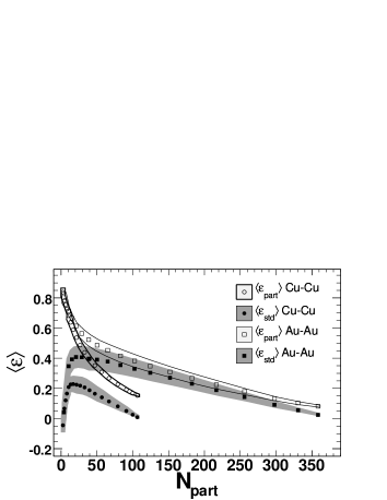
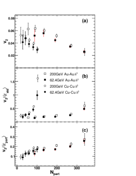
Figure 6: (top) Standard and participant eccentricity for Au+Au and Cu+Cu collision vs. $N_{part}$. (bottom) $v_{2}$, $v_{2}/\epsilon_{std}$, and $v_{2}/\epsilon_{part}$ for Au+Au and Cu+Cu collisions at 200 and 62.4 GeV, from PHOBOS.

The top panel of Fig. 6 shows $\epsilon_{std}$ as a function of $N_{part}$, and illustrates how it goes to 1 for small $N_{part}$ and large $N_{part}$. While there is no principle requiring $v_{2}$ to be linear with $\epsilon_{std}$, it turns out to be in all numerical calculations. The same hydrodynamic calculations suggest that there is a maximum value of $v_{2}/\epsilon$, which has been called the “hydrodynamic limit” reflecting that full equilibrium is reached [22]. Again, there is no known deep principle behind this concept, as it arises out of the interplay of transverse pressure and longitudinal expansion. However, all of this does suggest that $v_{2}/\epsilon$ is an important diagnostic variable which removes the “trivial” contribution from the overlap geometry and provides access to the magnitude of the pressure build-up, and thus potentially to the equation of state [7].

Experimental data from several collision energies, and a range of collision centralities shows that the “pressure”, as diagnosed via $v_{2}/\epsilon$ is a simple near-linear function of $dN/dy/\langle S\rangle$, where $S\equiv\pi\sigma_{X}\sigma_{Y}$ is the transverse area of the initial matter distribution [23]. This suggests that the pressure is a function of the entropy density in the transverse plane (if multiplicity is generally thought to be linear with the entropy, as will be discussed more later). Of course, it is observed that the data rises monotonically with transverse density, or (almost) equivalently with $N_{part}$ as shown for Au+Au in the lower panels of Fig. 6. It appears that the “hydrodynamic limit” has been observed yet, although it has been argued by some authors that this indicates the approach to equilibration, rather than equilibration itself [24]. The current experimental and theoretical situation precludes definitive statements either way, but at the very least it appears to be universal across changes in both energy and geometry (two ways to the edge of liquidity, or fluidity). It also does not seem to be “broken” even in very peripheral events or at low energies, where one might expect the low multiplicities to not favor local equilibration.

One way to probe the limits of this picture is to thus go to much smaller systems, Cu+Cu collisions for example, which reduce the number of participating nucleons by a factor of three. Data on $v_{2}$ as a function of $N_{part}$, shown in the lower panels of Fig. 6, already shows that these systems appear very different. The Au+Au data has a maximum $v_{2}$ at $N_{part}\sim 100$ and decreases to 1-2% at $N_{part}\sim 350$. Conversely, the Cu+Cu data starts at 4-5% and only decreases to 3% in the most central collisions. Already this looks very strange, since by construction, $\epsilon_{std}\rightarrow 0$ for the most central events. How can central Cu+Cu have so much apparent transverse pressure when there is presumably no geometric way to generate it? Things are even more confusing when plotting $v_{2}/\epsilon_{std}$ as a function of $N_{part}$ for Au+Au and Cu+Cu. There seems to be no connection between these two systems. Theoretical calculations typically assume that the matter density is a smoothly varying one, described by a Fermi distribution.However, experiments and many dynamical models assume that interactions occur by nucleon-nucleon collisions where individual nucleons are distributed uniformly throughout the nuclear volume, e.g. as implemented by “Glauber Monte Carlo” approaches[25]. The finite number, both in Cu and Au nuclei, lead to fluctuations in the matter density which are especially notable in peripheral Au+Au and nearly all Cu+Cu collisions. If one assumes the matter density is not defined by an idealized overlap zone of the nuclear densities, but by the distribution of the participants themselves, then the correct scaling should be achieved using what is called the “participant eccentricity” as first defined by PHOBOS [26]

$$\epsilon_{part}=\frac{\sqrt{(\sigma^{2}_{Y}-\sigma^{2}_{X})^{2}+4(\sigma^{2}_{XY})^{2}}}{\sigma^{2}_{X}+\sigma^{2}_{Y}}$$ (4)

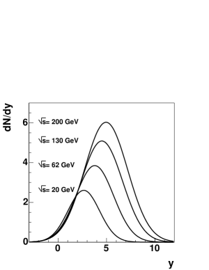
Figure 7: Extended longitudinal scaling in Landau’s hydrodynamics, from Ref.[29]

This measures the shape of the region defined by the principal axes of the participants, on an event-by-event basis, using a Glauber Monte Carlo calculation. This quantity has the advantage over $\epsilon_{std}$ of being positive definite for all values of impact parameter. Thus, $\epsilon_{part}$ does not necessarily trend to zero for $b\rightarrow 0$, which is now understood as being due to fluctuations.

Scaling $v_{2}$ for several collision energies, centralities, and system sizes by $\epsilon_{part}$ shows a universal scaling of $v_{2}/\epsilon_{part}$ with $dN/dy/\langle S\rangle$, or similarly $N_{part}$ as shown in Fig. 6. This suggests that the geometrical configuration of the participants (at least as indicators for the spatial location of inelastic interactions) is “frozen in” immediately, i.e. it does not require substantial time for the deposited energy to locally equilibrate and react hydrodynamically. This is of course fully consistent with the previous estimates of $\tau_{0}$, but suggests that there is little room for “free streaming” before thermalization [7].

4 Initial Conditions

Rapid equilibration in strong interactions is a physical scenario with a long history[6, 27]. Landau and Fermi considered this possibility in the early 1950’s when estimating the total multiplicity generated in the collision of two nuclei, or even nucleons, by estimating the total entropy assuming all of the incoming energy is thermalized in a Lorentz-contracted volume. In the hydrodynamic paradigm, the strength of the interactions leaves no natural scales in the problem save two, 1) the initial longitudinal size and thus the time scale $\tau_{0}\propto\Delta z\propto 1/\gamma\propto 1/\sqrt{s}$, and the final temperature, or equivalent density, described above [28]. As described in several recent references (e.g. Ref. [29], these initial conditions lead to testable phenomenological consequences. The multiplicity in the Fermi-Landau approach scales as $N\propto s^{1/4}$, a power-law behavior that is compatible with a wide variety of total multiplicity data from a variety of systems over several orders of magnitude in beam energy. It leads to Gaussian rapidity distributions with variance $\sigma^{2}_{y}=\ln(\sqrt{s}/2m)$ [28]. Combining these two formulae leads to particle densities that approximately scale when viewed in the rest frame of one of the projectiles, as a functionn of $\eta-y_{\mathrm{beam}}$, as shown in Fig. 7.

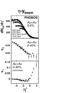
Figure 8: Extended longitudinal scaling seen in PHOBOS data on $dN/d\eta/N_{part}/2$

Landau’s initial conditions and dynamical evolution are in some sense very different than the one suggested by Bjorken in the early 1980’s, where “boost-invariance” was thought to be the relevant feature of the dynamics of strong interactions [20]. Boost-invariance is in fact a generic feature of hydrodynamic solutions, and was noticed by Landau in his hydrodynamic calculations [9]. In general, the difference between the two is a matter of evolution time and Landau’s initial conditions have a much different causal structure. Early thermalization in the highly compressed initial state leads to strong longitudinal expansion controlled by $\tau_{0}$. Conversely, boost-invariant initial conditions lead to no longitudinal pressure gradients, but simply $v=z/t$ (a la like Hubble expansion).

RHIC data do not show any clear signs of boost invariance in the final state. Intead they have a strong rapidity dependence [30], also seen by the elliptic flow as a function of pseudorapidity [31]. Interestingly, they also show an invariance when plotted as a function of $\eta-y_{beam}$, shown in Fig. 8 from Ref. [32]. for $dN_{ch}/d\eta$, $v_{2}$ and $v_{1}$, circumstantial evidence that particle production in heavy ion collisions undergoes early thermalization and thus strong longitudinal expansion.

It then becomes an interesting question whether all of these scaling relations indicate a broader validity of the near-perfect fluid paradigm over most the collision evolution. The scaling relations hold as a function of energy, centrality, and rapidity. They are thus related to the question of thermalization time and its effects on longitudinal dynamics.

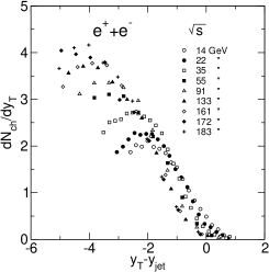
Figure 9: Extended longitudinal scaling seen in $e^{+}e^{-}$ reactions, from Ref. [3].

This points directly to an even deeper question, that of whether or not there is a dynamical length scale in the problem: one that reflects the microscopic dynamics than simply the boundary conditions. If no such scale exists, then there is no natural way to argue that some systems, e.g. nucleon-nucleon collisions or $e^{+}e^{-}$ annihilation into hadrons, are “too small” to rapidly thermalize or react hydrodynamically. Those systems have been noted to have the same multiplicity (i.e. entropy) [33] and freezeout temperature [34] as nominally larger systems, and they also have been long-known to show extended longitudinal scaling [3, 35]. It is conceivable that all strong interactions could be understood in part by the near-perfect fluid paradigm. The criticism that $e^{+}e^{-}$ is already understood via perturbative QCD calculations can be countered by the fact that these calculations seem to show features that are parametrically similar to Landau’s hydrodynamic model[36, 37]. In the end, all of this will hinge on the viscosity of the produced matter, something which will be discussed below.

5 Degrees of Freedom

And yet, even if the near-perfect fluid paradigm is relevant over most of the evolution, one major outstanding question remains. What is the fluid made of? How did it come into being as a locally equilibrated state of matter?

Figure 10: Data on $v_{2}$ vs. $p_{T}$ compared to various equations of state, from Ref. [38].

Obviously there must be some non-equilibrium dynamics to generate the observed entropy. Nothing in the data discussed so far uniquely indentifies which degrees of freedom are able to achieve this. The most natural assumption would be that the early stages are dominated by the dynamics of free quarks and gluons, or at least the dynamics of quark and gluon fields that are studied using Lattice QCD. However, attempts to model the existing data on $v_{2}$ vs. $p_{T}$ for identified particles find that a first-order phase transition needs to be put in by hand [38]. The existing calculations, shown in Fig. 10 do not provide sufficient “softening” of the equation of state to model the heavier particles which are most sensitive to the speed of sound.

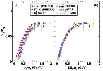
Figure 11: PHENIX data on $v_{2}$ for different particle species, scaled by the number of constituent quarks ($n_{q}$), from Ref. [39].

These data have been studied for many different particles species, which have different mass and quark content. Recent PHENIX data [39] shows that all of the available data on $v_{2}$ vs. $p_{T}$ lie near one another when plotted as a function of $v_{2}/n_{q}$ on the Y axis, where $n_{q}$ is the number of valence quarks and anti-quarks in the hadron, and $KE_{T}/n_{q}$ on the X axis, where $KE_{T}=m_{T}-m$ for each hadron of mass $m$. This suggests a scenario where freezeout occurs by the recombination of “constituent quarks”, particles which have a mass of $\sim m/n_{q}$ and the right quantum numbers for each hadron. However, the same PHENIX paper also suggests that “the scaling with valence quark number may indicate a requirement of a minimum number of objects in a localized region of space that contain the prerequisite quantum numbers of the hadron to be formed. Whether the scaling further indicates these degrees of freedom are present at the earliest time is in need of more detailed theoretical investigation”. If one considers the overall dynamical evolution of the system, with many independent stages in principle [37], it is possible that constituent quark scaling is only probing the very final stages before formation of the final state hadrons. Thus, it is premature to suggest that these RHIC data gives direct information about the early-time formation of a truly quark and gluon phase.

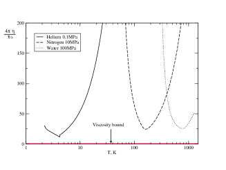
Figure 12: $4\pi\eta/s$ for a variety of systems, with the postulated lower bound indicated, from Ref. [41].

Suggesting that quasi-free quarks and gluons are not the active degrees of freedom at early times does not obviously contradict lattice data. In most calculations it is found that $\epsilon/T^{4}$, which is proportional to the thermodynamically-active number of degrees of freedom, does not approach the Stefan-Boltzmann limit even at high temperatures. In fact it falls short of the limit by about 20%. AdS/CFT-based arguments, which model the strongly-coupled Yang-Mills plasma as a 10 dimensional black hole, predict precisely a 25% shortfall in the number of degrees of freedom [40]. Similar arguments have also shown that the shear viscosity on the gauge theory side is proportional to the entropy density, and their ratio has a lower bound [41], i.e. $\frac{\eta}{s}\geq\frac{1}{4\pi}$.

It is now an active field of investigation to understand the precise mechanism which implements strong coupling in QCD. Shuryak, Zahed, Brown and others have proposed the presence of colored bound states in a QCD plasma [42, 43]. This leads to larger cross sections and thus stronger coupling in the system. And yet, similar lattice calculations, as discussed above, find that the fluctuations of quark-antiquark fields are not consistent with the active degrees of freedom being $q\overline{q}$ bound states [44, 45].

Conventional fluids, shown in Fig. 12 exceed the postulated viscosity bound by a factor of ten [41]. The success of the hydrodynamic models shown above suggests that the viscosity is almost negligible, possibly saturating the bound or even being essentially zero. And yet, the precise value of $\eta/s$ has not been established using experimental data. It is clear that saturating the viscosity bound would make an exciting connection between relativistic heavy ion collisions and a prediction based on physics nominally far from the original domain of RHIC physics.

6 The Future

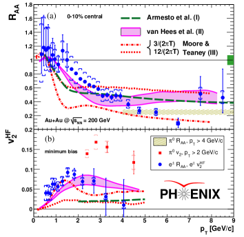
Figure 13: PHENIX data [46] on charm suppression and elliptic flow for Au+Au collisions.

Probing the transport properties of the system will be the focus of the next generation of RHIC experiments. A natural probe of this is the transport of heavy quarks. New silicon detectors in PHENIX and STAR are being developed to measure charmed particles by means of displaced decay vertices. By studying the correlation between the flow and energy loss of charmed mesons, e.g. from recent PHENIX data [46] shown in Fig. 13, it is possible to relate their magnitude to a charm diffusion coefficient $D$ [47]. This in turn allows an estimation of shear viscosity by the Einstein relation $D\sim 6\eta/sT$. Already a first measurement of this quantity has been performed by PHENIX, which suggests the viscosity seen by charm quarks falls at most within a factor of 2-3 above the viscosity bound. The next generation of measurements should substantially improve the experimental precision.

At the same time, theoretical calculations will also have make equivalent strides. Fully three-dimensional hydrodynamical calculations will be required, with full control over initial conditions and freezeout (e.g. Ref. [48]). All possible initial conditions, from Landau’s to Bjorken’s should be accessible. This should be coupled with truly systematic studies in order to assign error bars to extracted parameters characterizing the initial state, equation of state, and freezeout conditions. Then we will have a quantitative handle on just how near we are to the most-perfect fluid.

The author would like to thank to the GHP organisers for the invitation to speak in Nashville. Thanks go my RHIC colleagues, as always, for useful comments and suggestions on the talk and proceedings, especially Mark Baker, Wit Busza, Jamie Nagle,Paul Stankus and Bill Zajc. This work was supported in part by the Office of Nuclear Physics of the U.S. Department of Energy under contracts: DE-AC02-98CH10886.

References

-
[1]
ttp://www.bnl.gov/bnlweb/pubaf/pr/PR_display.asp?prID=05-38 }
\bibitem{Arsene:2004fa} Arsene I {\it et al.} 2005  {\it Nucl.\ P
ys. A 757 1 - [2] Adcox K et al. 2005 Nucl. Phys. A 757 184
- [3] Back B B et al. 2005 Nucl. Phys. A 757 28
- [4] Adams J et al. 2005 Nucl. Phys. A 757 102
-
[5]
ttp://www.aip.org/pnu/2005/split/757-1.tml - [6] Landau LD 1953 Izv. Akad. Nauk Ser. Fiz. 17 51
- [7] Kolb P F and Heinz U 2003 arXiv:nucl-th/0305084.
- [8] Boyd G et al 1996 Nucl. Phys. B 469 419
- [9] Belenkij S Z and Landau L D 1956 Nuovo Cim. Suppl. 3S10 15
- [10] Cooper F, Frye G and Schonberg E 1974 Phys. Rev. Lett. 32 862
- [11] Hagedorn R 1965 Nuovo Cim. Suppl. 3 147
- [12] Back B B et al. 2006 arXiv:nucl-ex/0610001
- [13] Braun-Munzinger P, Redlich K and Stachel J arXiv:nucl-th/0304013.
- [14] Cleymans J and Redlich K 1998 Phys. Rev. Lett. 81 5284
- [15] Back B B et al. 2002 Phys. Rev. Lett. 89 222301
- [16] Kolb P F, Sollfrank J and Heinz U W 1999 Phys. Lett. B 459 667
- [17] Voloshin S and Zhang Y 1996 Z. Phys. C 70 665
- [18] Back B B et al. 2005 Phys. Rev. C 72 051901
- [19] Kolb P F, Huovinen P, Heinz U W and Heiselberg H 2001 Phys. Lett. B 500 232
- [20] Bjorken J D 1983 Phys. Rev. D 27 140
- [21] Ollitrault J Y 1992 Phys. Rev. D 46 229
- [22] Voloshin S A and Poskanzer A M 2000 Phys. Lett. B 474 27
- [23] Adler C et al. 200 Phys. Rev. C 66 034904
- [24] Bhalerao R S, Blaizot J P, Borghini N and Ollitrault J Y 2005 Phys. Lett. B 627 49
- [25] Miller M L, Reygers K, Sanders S J and Steinberg P 2007 arXiv:nucl-ex/0701025
- [26] Manly S et al. 2006 Nucl. Phys. A 774 523. Alver B et al. 2006 arXiv:nucl-ex/0610037.
- [27] Fermi E 1950 Prog. Theor. Phys. 5 570
- [28] Carruthers P 1974 Annals N.Y.Acad.Sci. 229 91
- [29] Steinberg P 2005 Acta Phys. Hung. A 24 51
- [30] Back B B et al. 2006 Phys. Rev. C 74 021901
- [31] Back B B et al. 2005 Phys. Rev. Lett. 94 122303
- [32] Roland G et al. 2006 Nucl. Phys. A 774 113
- [33] Back B B et al. 2006 Phys. Rev. C 74 021902
- [34] Becattini F, Gazdzicki M and Sollfrank J 1998 Eur. Phys. J. C 5 143
- [35] Alner G J et al. 1986 Z. Phys. C 33 1
- [36] Tesima K 1990 Z. Phys. C 47 43
- [37] Steinberg P 2005 Nucl. Phys. A 752 423
- [38] Huovinen P 2005 Nucl. Phys. A 761 296
- [39] Adare A et al. 2006 arXiv:nucl-ex/0608033
- [40] Gubser S S, Klebanov I R and Peet A W 1996 Phys. Rev. D 54, 3915
- [41] Kovtun P, Son D T and Starinets A O 2005 Phys. Rev. Lett. 94 111601
- [42] Shuryak E V and Zahed I 2004 Phys. Rev. D 70 054507.
- [43] Brown G E, Lee C H, Rho M and Shuryak E 2004 Nucl. Phys. A 740 171
- [44] Majumder A, Koch V and Randrup J 2005 J. Phys. Conf. Ser. 27 184
- [45] Karsch F, Ejiri S and Redlich K 2005 Nucl. Phys. A 774 619
- [46] Adare A 2006 arXiv:nucl-ex/0611018.
- [47] Moore G D and Teaney D 2005 Phys. Rev. C 71 064904
- [48] Hirano T and Nara Y 2004 Nucl. Phys. A 743 305