Identified hadron transverse momentum spectra
in Au+Au collisions at $\sqrt{s_{{}_{NN}}}$=62.4 GeV

Abstract

Transverse momentum spectra of pions, kaons, protons and antiprotons from Au+Au collisions at $\sqrt{s_{{}_{NN}}}$ = 62.4 GeV have been measured by the PHOBOS experiment at the Relativistic Heavy Ion Collider at Brookhaven National Laboratory. The identification of particles relies on three different methods: low momentum particles stopping in the first detector layers; the specific energy loss ($dE/dx$) in the silicon Spectrometer, and Time-of-Flight measurement. These methods cover the transverse momentum ranges 0.03–0.2, 0.2–1.0 and 0.5–3.0 GeV/c, respectively. Baryons are found to have substantially harder transverse momentum spectra than mesons. The $p_{T}$ region in which the proton to pion ratio reaches unity in central Au+Au collisions at $\sqrt{s_{{}_{NN}}}$ = 62.4 GeV fits into a smooth trend as a function of collision energy. At low transverse momenta, the spectra exhibit a significant deviation from transverse mass scaling, and when the observed particle yields at very low $p_{T}$ are compared to extrapolations from higher $p_{T}$, no significant excess is found. By comparing our results to Au+Au collisions at $\sqrt{s_{{}_{NN}}}$ = 200 GeV, we conclude that the net proton yield at midrapidity is proportional to the number of participant nucleons in the collision.

I Introduction

The yield of identified hadrons produced in collisions of gold nuclei at an energy of $\sqrt{s_{{}_{NN}}}$ = 62.4 GeV has been measured with the PHOBOS detector at the Relativistic Heavy Ion Collider (RHIC) at Brookhaven National Laboratory. The data are presented as a function of transverse momentum, transverse mass, and centrality.

It was shown previously by PHOBOS that, the inclusive charged hadron transverse momentum spectra in Au+Au collisions exhibit the same centrality dependence at center-of-mass energies of $\sqrt{s_{{}_{NN}}}$ = 200 GeV and 62.4 GeV Back et al. (2005a). It is also known that in central Au+Au collisions at 200 GeV Adler et al. (2004a) and 130 GeV Adcox et al. (2002a, 2004), the proton and antiproton yields become comparable to the pion yields above $p_{T}\approx 2$ GeV/c. The yield of high-$p_{T}$ particles has been measured to be suppressed with respect to the scaling with the number of binary nucleon-nucleon collisions Adcox et al. (2002b, 2003); Adler et al. (2004b, 2002); Adams et al. (2003); Arsene et al. (2003); Back et al. (2004a), but that suppression was found to be strongly species-dependent Adler et al. (2004a).

The present study at 62.4 GeV aims to extend the energy range for which the contributions of different particle species to the inclusive charged hadron spectra are known. These results add to our knowledge of the energy dependence of baryon transport and baryon production in heavy-ion collisions, and of parton energy loss in the hot and dense medium Gyulassy and Plumer (1990), that is believed to be produced.

The results presented here allow the first examination of differences between the transverse dynamics of various particle species at 62.4 GeV, bridging a gap between the top SPS energy ($\sqrt{s_{{}_{NN}}}$=17.2 GeV) and the higher RHIC energies (130 and 200 GeV). This is the first publication using the PHOBOS Time-of-Flight detector for particle identification, and using the PHOBOS silicon Spectrometer to obtain momentum spectra of identified particles.

II The PHOBOS Detector

Figure 1: The layout of the PHOBOS detector system used in the Au+Au run at 62.4 GeV. The silicon Spectrometer arms are located in the center, placed in a double dipole magnetic field. The two Time of Flight scintillator walls (center-top of the figure) detect particles emitted near 45 and 90 degrees from the beam direction and are located at a distance to the collision point of 5.34 and 3.80 meters, respectively.

The PHOBOS detector Back et al. (2003a) is designed to provide global characterisation of heavy-ion collisions, with about 1% of particles analyzed in detail in the Spectrometer system. The layout of the PHOBOS detector system is shown in Fig. 1. Only the parts of the detector relevant to the present analysis will be described.

II.1 Event Trigger and Vertex-finding

The primary event trigger requires a coincidence between the ‘Paddle Counters’ Bindel et al. (2001), which are two sets of sixteen scintillator detectors located at $z=\pm 3.21$ m (where $z$ is the distance from the nominal collision point along the beam direction) and spanning the pseudorapidity region $3.2\leq|\eta|\leq 4.5$.

The Zero-Degree Calorimeters (ZDCs) Adler et al. (2003), positioned at $\pm 18$ m, measure spectator neutrons from the collision. With an identical design for each of the four RHIC experiments, the ZDCs are built from tungsten optical-fibre sandwiches. A requirement of a ZDC coincidence can be added to the event trigger to enhance trigger purity in high background situations.

An online vertex is determined with a resolution of roughly $4$ cm using the Time-Zero (T0) detectors, two sets of ten Čerenkov radiators situated close to the beam pipe, at $z=\pm 5.2$ m. This vertex trigger enhances the fraction of recorded events in the vertex region in which the efficiency of the PHOBOS Spectrometer is maximal, $-20\leq z\leq 20$ cm.

Offline vertex reconstruction makes use of information from different sub-detectors. Two sets of double-layered silicon Vertex Detectors are located below and above the collision point. PHOBOS also has two Spectrometer arms in the horizontal plane used for tracking and momentum measurement of charged particles. For events in the selected vertex region, the most accurate $z$ and $y$ (vertical) positions are obtained from the Vertex Detector, while the position along $x$ (horizontal, perpendicular to the beam) comes primarily from the Spectrometer. The final resolution of the vertex position along $z$ is found to be better than 300 $\mu$m.

II.2 Particle Tracking and Identification Detectors

Particle tracking and identification in the PHOBOS experiment is performed using the Spectrometer and the Time-of-Flight (TOF) system.

Each arm of the Spectrometer consists of 137 silicon pixel sensors arranged into layers, with an azimuthal angular coverage of $\Delta\phi\approx 0.1$ radians. The silicon sensor technology used in the PHOBOS detector is described in Nouicer et al. (2001). The Spectrometer sensors are designed to give precise hit position determination in the $x-z$ plane.

The first silicon layer is positioned within 10 cm from the interaction point, allowing good rejection of tracks from displaced vertices. The thickness of the beam-pipe is 1 mm, and it is constructed from beryllium to minimise multiple scattering and secondary particle production.

The PHOBOS double-dipole magnetic field is designed such that the inner six Spectrometer layers sit in a low-field region while the remaining layers are in an approximately constant vertical magnetic field of 2 T.

There are two TOF walls: Wall B, centered around a line at 45^o to the beam-line and located 5.4 m from the origin; and Wall C, also facing the collision point, but centered around a line at 90^o to the beam-line, at a distance of 3.9 m. Each wall consists of 120 vertical Bicron BC-404 plastic scintillator rods which are 20 cm long with a cross-section of 8$\times 8$ $mm^{2}$. The scintillators have PMT read-out top and bottom, providing vertical position information. The present analysis uses only data from TOF Wall B, due to low statistics in Wall C for the short 62.4 GeV run.

Particle timing information is obtained relative to an event ‘start-time’ determined from the T0 Čerenkov detectors. Leading edge discriminators are used, therefore slew corrections of the timing signals as a function of pulse height are necessary. The stability of the timing signals arriving at the TDCs over long cables is monitored and drifts caused by temperature changes are corrected for. Channel-by-channel cable delay differences are corrected using TOF hits matched to tracks reconstructed in the Spectrometer with known momenta. A similar adjustment is accomplished for the T0 detectors using the signals originating from the prompt (fastest) particles close to the beam direction. The combined T0-TOF system was found to have a total timing resolution of about 140 ps.

III Event Selection and Centrality

The events selected for analysis were divided into three centrality classes, based on signals in the Paddle detectors. The mean number of participating nucleons ($\langle{\rm N_{part}}\rangle$) and the mean number of binary nucleon-nucleon collisions ($\langle{\rm N_{coll}}\rangle$) were estimated for each centrality class using Monte-Carlo methods. These $\rm{N_{part}}$ and $\rm{N_{coll}}$ values and their systematic errors are listed in Table 1. Details of the estimation procedure and the selection of events can be found in Appendix A.

Centrality	$\left<N_{part}\right>$	$\left<N_{coll}\right>$
30–50%	$88\pm 9$	$128\pm 17$
15–30%	$175\pm 9$	$331\pm 23$
0–15%	$294\pm 10$	$684\pm 23$
0–50%	$176\pm 9$	$356\pm 21$

Table 1: Details of the centrality classes used in this analysis. Bins are expressed in terms of percentage of the total inelastic Au+Au cross-section at $\sqrt{s_{{}_{NN}}}$=62.4 GeV.

IV Track Reconstruction and Particle Identification

The present analysis uses essentially the same Spectrometer tracking procedures as previously applied to obtain non-identified charged hadron spectra results from PHOBOS Back et al. (2004b, 2003b, c, 2005a). Details are given in Appendix B.

Three independent methods were used for particle identification, over differing momentum ranges.

The charged particle yields at very low momentum were measured by searching for particle tracks that stop in the $5^{\rm th}$ spectrometer layer. This technique allows identification of pions between 0.03 and 0.05 GeV/c, kaons between 0.09 and 0.13 GeV/c, and protons between 0.14 and 0.21 GeV/c transverse momentum, close to mid-rapidity ($-$0.1$<$y$<$0.4). The procedure is summarized in Appendix C, with further details presented in Back et al. (2004d).

For particles at intermediate momentum, the velocity-dependent specific energy loss ($dE/dx\propto 1/v^{2}$) in the silicon Spectrometer can be used to separate particles with the same momentum but different mass. A truncated mean calculation is used, discarding the 30% highest energy hits on each reconstructed Spectrometer track. This reduces the effect of the large Landau tails of the energy-loss distribution and improves sensitivity for particle identification. Previous PHOBOS publications of antiparticle to particle ratios using $dE/dx$ identification Back et al. (2001); Back et al. (2003c, 2004e); Back et al. (2005b) made cuts in $dE/dx$ versus total momentum $p$ to identify particles. In the present analysis, however, to extend the range for identification, particle yields were extracted as a function of momentum by fitting the $dE/dx$ distributions. This is illustrated in Fig. 2 and details are discussed in Appendix C. This technique allows particle identification in the momentum ranges $0.2<p<0.9$ GeV/c for pions and kaons, and $0.3<p<1.4$ GeV/c for protons and antiprotons.

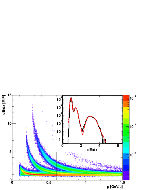
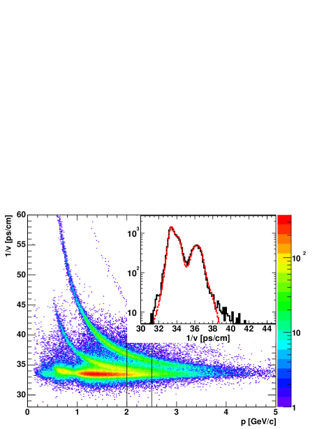
Figure 2: (Color online) Top panel: $dE/dx$ in the silicon spectrometer as a function of total momentum. Bottom panel: inverse velocity of particles in the TOF detector as a function of momentum. Insets: the spectra are fitted to obtain raw particle yields. From left to right: pions, kaons and protons are shown (positive charges). The lines indicate the selected momentum slice to plot the insets.

Finally, between 0.5 and 3 GeV/c transverse momentum, the Time of Flight detector system was used to measure the velocity. The identification is based on the simultaneous determination of the velocity and the momentum of these particles. Details are summarized below.

The magnetic field of the PHOBOS magnet was carefully measured outside of the dipole gaps (far from the beam line, up to the TOF walls), as well as modeled with numerical calculations based on the electric current and detailed coil and magnet yoke geometry and materials. The good agreement between measurements and the calculation made it possible to project the particle tracks measured by the Spectrometer (where the last Si layer is situated at about 1 m distance from the collision point) to the TOF walls (at 4-5 m from the collision point) with good precision. The hits in the TOF and the charged particle tracks were matched, and the path lengths of the trajectories were calculated with better than 1 cm accuracy. The time difference between the TOF and the T0 signal, after corrections for cable length differences, drifts caused by temperature changes, slewing and channel-by-channel delay corrections provided the flight time of the particle. The inverse velocity was then calculated for each track, and plotted as a function of the particle momentum measured by the Spectrometer (shown by the bottom panel of Fig. 2).

Within a given momentum bin, the trajectories corresponding to different species are similar, therefore the path lengths do not vary significantly. The TOF timing signal, after slewing corrections, is not sensitive to the particle mass. The path length error is negligible compared to the timing error multiplied by the speed of light. For these reasons, the inverse velocity ($1/v$) resolution is directly proportional to the timing resolution (combined from the contributions of the T0 and TOF detectors) and independent of the particle mass.

The $1/v$ distributions in momentum bins were analyzed in a very similar way to the $dE/dx$ distributions. The line shape for a given species was a Gaussian complemented with a small tail to account for the non-Gaussian nature of the timing error. The mean of the Gaussian was given by $1/v=\sqrt{m^{2}/p^{2}+1/c^{2}}$. In each total momentum bin with finite width, the spread of the velocity values according to this formula was taken into account by convoluting the resolution function with the calculated velocity distribution in the momentum bin. The width of the resolution function was constant for all species and momenta. The only free fit parameters were the amplitudes (particle yields) corresponding to the three hadron species. The fit functions created this way describe the data well, as shown in the inset on the bottom panel of Fig. 2.

In the high $p_{T}$ region, where the kaons and pions cannot be separated any more, only the meson yield (the sum of kaon and pion yield) and the proton yield was measured. For the purpose of constructing the meson line shape, the kaon/pion ratio was extrapolated from the lower momentum region. For example, the $K^{+}/\pi^{+}$ ratio that was measured to be about 0.65 at $p_{T}=1.2$ GeV/c was extrapolated to a range between 0.8 and 2.6 at 3 GeV/c. The lack of precise knowledge of that ratio influences the measured proton yield, causing a small systematic error which was estimated to be 2–4%.

The above fits were performed in total momentum bins for both charge signs and both magnetic field settings separately.

V Corrections

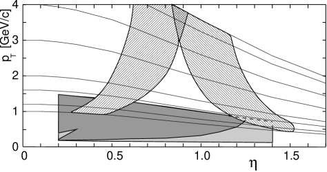
Figure 3: Acceptance of the data used in this analysis in the $(p_{T},\eta)$ plane. The two branches at high $p_{T}$ represents the TOF, while the shaded areas at lower $p_{T}$ represent the Si spectrometer acceptance, for the two bending directions (note that the latter for one bending direction contains the other). The thin lines are drawn at constant total momentum values.

Detector-effects need to be unfolded from the measured distributions in order to obtain the true transverse momentum spectra for identified particles. The various corrections compensate for geometrical acceptance and tracking efficiency; occupancy in Spectrometer; ghost tracks; momentum resolution; feed-down from weak decays of the $\Lambda$ and $\Sigma$ particles; secondary particles originating from the detector material; and dead channels in the various detectors. The details of the above corrections are discussed in Appendix D.

VI Combining $dE/dx$ and TOF data

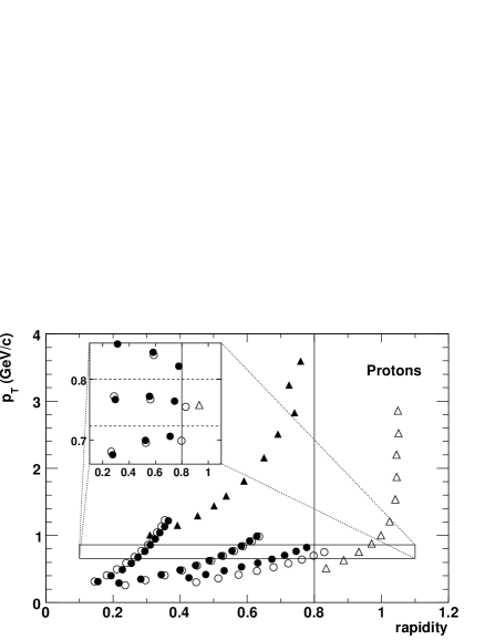
Figure 4: Location of PID data-points in $(p_{T},y)$-space, for protons from the most central bin. Triangles represent TOF, while circles correspond to Spectrometer data that was sliced into three $\eta$ bins. Open and closed symbols differentiate between bending directions. The line at $y=0.8$ indicates the chosen common rapidity value at which all invariant particle yields will be evaluated. The inset shows a subset of the same points on a different scale, where the horizontal dashed lines enclose an example set of data points that will be merged and quoted with a single $p_{T}$ value.

Because of the dipole magnet configuration and the fixed position of the TOF wall, the various particle species are detected in slightly different rapidity regions in the TOF wall, depending on their transverse momentum. The geometrical acceptance for the identification in the TOF walls and in the silicon spectrometer for the three species and two magnet polarities are illustrated in Fig. 3 in $(p_{T},\eta)$-space. To provide for an easier comparison of our data to theoretical models or other experiments, we synthesize the results from these different acceptances to generate the $p_{T}$ spectrum for each species at a constant rapidity.

The Spectrometer data is divided in three bins in pseudorapidity, $0.2\leq\eta<0.6$, $0.6\leq\eta<1.0$ and $1.0\leq\eta\leq 1.4$. Particle identification is performed in bins of total momentum $p$; the rapidity for each species is calculated from the mean $p$ and $p_{T}$ in each (p,$\eta$) bin, and the location of the data-points is plotted in $(p_{T},y)$-space. An example is shown for protons in Figure 4, with an inset which details the region around $p_{T}=0.75$ GeV/c. From these plots a common rapidity value is chosen (vertical line at $y=0.8$); the invariant yield at this rapidity is evaluated for the whole $p_{T}$ range, using the data measured at different rapidities.

The procedure to synthesize all of the data for a particular species into a $p_{T}$ spectrum at $y=0.8$ begins by choosing data-points which are close in $p_{T}$. An example of such a small $p_{T}$ region is shown in the inset of Figure 4 by the two horizontal dashed lines. The seven data points falling between the lines will be combined in the following way. The invariant yield, $Y=\frac{1}{2\pi p_{T}}\frac{d^{2}N}{dp_{T}dy}$, of all points in the selected region is plotted versus rapidity (see Fig. 5). The simplest assumption is that the invariant yield is constant over the measured narrow rapidity interval near mid-rapidity. We therefore take the best constant fit to these points as the value of the invariant yield at this $p_{T}$. For comparison, we also fit a straight line to the points; the difference between the constant fit and this straight line evaluated at the common rapidity point is taken as a measure of the systematic error introduced by this assumption. This process is illustrated for a single $p_{T}$ ‘slice’ in Figure 5. The statistical error on the synthesized invariant yield is the propagated error from the individual points (shown by small horizontal bars).

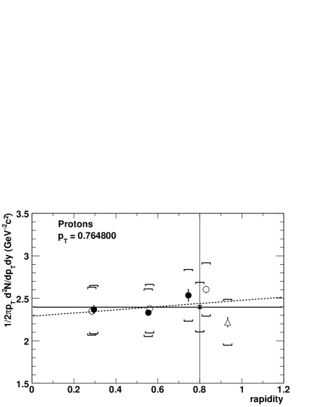
Figure 5: Example of the synthesis of TOF and $dE/dx$ data. The invariant yield is plotted versus rapidity for protons from central collisions, at $p_{T}=0.765$. The statistical errors on each point are shown by bars, and the brackets represent the systematic errors. The thick solid and dashed lines show the best constant and straight-line fits to these points. The vertical line is the common rapidity value; the brackets on this line represent the total systematic error on the synthesized invariant yield.

An important consideration in finding the yields which are fit as shown in Figure 5 is the fact that, although the data-points have similar $p_{T}$ values, they are not identical. Therefore, it is necessary to account for the strong $p_{T}$ dependence of the particle yields. This is done using a Taylor expansion:

$$f(p_{T}+\Delta p_{T})\approx f(p_{T})+\Delta p_{T}\frac{df(p_{T})}{dp_{T}}$$ (1)

where $f(p_{T})$ is the yield of an individual data point and $\Delta p_{T}$ is the difference between the $p_{T}$ of that point and the average $p_{T}$ of all points being combined. The slope of the $p_{T}$-dependence, $\frac{df(p_{T})}{dp_{T}}$, is found by doing a fit to all of the raw data points for a particular bending direction (i.e. either the open or closed symbols in Figure 4), ignoring for the moment that each of these points is at a different rapidity. The yield of each individual data point is ‘perturbed’ in this way to a common $p_{T}$ value before they are merged to find the yield at $y=0.8$. In principle, this adjustment of the data points could be iterated using the spectrum found after projecting to $y=0.8$ in order to obtain a more precise value of the slope, $\frac{df(p_{T})}{dp_{T}}$. In practice, however, the applied shifts were so small that such a refinement was unnecessary.

VII Integrating the ${\rm p_{T}}$ Spectra

Proton and antiproton $d^{2}N/dp_{T}dy$ transverse momentum distributions were integrated to obtain the total particle yield $dN/dy$. We integrate over the measured data points and extrapolate over the unmeasured low-$p_{T}$ region. Because the $p_{T}$ spectrum falls so sharply, the high-$p_{T}$ region beyond the measured points makes a negligible contribution to the total yield and is not included. The low-$p_{T}$ extrapolation uses a simple straight line from zero to the first data point; this result is compared to that obtained using a variety of physically-motivated fit functions.

Statistical errors on the integral turn out to be negligible. Systematic errors on the total yield come from propagation of the errors on the individual data-points, plus additional uncertainty which arises as a result of the extrapolation over the unmeasured low-$p_{T}$ region.

VIII Results

After all corrections are applied, the invariant yields ($d^{2}N/2\pi p_{T}dp_{T}dy$) of each species in the three centrality classes are plotted as a function of transverse momentum in Fig. 6, for Au+Au collisions at $\sqrt{s_{{}_{\rm NN}}}=62.4$ GeV. As described in the previous section, the final data is extracted at $y=0.8$ for all species, by combining the actual measurements from the $dE/dx$ and TOF identification methods, which cover the geometrical acceptance shown in Fig. 3.

Above a transverse momentum of 1.4 GeV/c, kaon yields cannot be distinguished from pions. The proton and antiproton yield can be measured up to $p_{T}=3$ GeV/c, where the limit is governed by the statistics of the data sample.

Systematic uncertainties on the invariant yields arise from various sources. The efficiency of track reconstruction and the acceptance of the Spectrometer carries a systematic error between 5 and 9%, decreasing with $p_{T}$. The feed-down correction for protons is estimated with a 4-8% precision, and this uncertainty also decreases at larger transverse momenta. There are several smaller error sources such as the feed-down to pions (1%), secondaries contributing to the proton yield (1%), dead channels in the Spectrometer (5%) and the TOF (2%), reconstructed ghosts/fakes (2%), the occupancy correction in the Spectrometer (3%) and the systematic error from the procedure to combine the data sets from different detectors (4-5%). Overall, the systematic uncertainty on the proton and antiproton yield is 14-16%, while for pions it is 13-15%, and 11-14% for kaons. For all species, the uncertainties decrease slightly with increasing transverse momentum out to $p_{T}\approx 2$ GeV/c and then rise slowly.

Figure 6: Transverse momentum spectra of $\pi^{+}$, $\pi^{-}$, $K^{+}$, $K^{-}$, $p$ and $\overline{p}$ particles for the three centrality classes in Au+Au collisions at $\sqrt{s_{{}_{NN}}}$=62.4 GeV. Left panels: positively-charged particles, right panels: negatively-charged particles.

Only a mild centrality dependence can be observed in the data, while the difference between the shapes of the $p_{T}$ spectra of various species is significant. At high transverse momenta, the proton and antiproton spectra become closely exponential in the measured $p_{T}$ range, while they flatten out at low $p_{T}$.

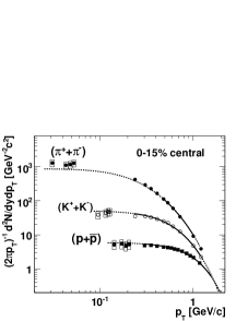
Figure 7: Blast-wave fits to identified particle spectra in Au+Au collisions at $\sqrt{s_{{}_{NN}}}=62.4$ GeV. Error bars represent statistical errors. Systematic errors are shown by the boxes for the data from the very low-$p_{T}$ analysis.

Figure 7 shows the comparison of these intermediate $p_{T}$ identified particle yields with the data at very low $p_{T}$, obtained from the analysis of particles stopping in the 5th active Si layer of the Spectrometer. The yields corresponding to the two charge signs for a particle were added here, since in the very low $p_{T}$ analysis it is not possible to determine the charge of the particle. A fit to the data was performed using a blast-wave parametrization Schnedermann et al. (1993). Each of $\pi^{+}$, $\pi^{-}$, $K^{+}$, $K^{-}$, $p$ and $\overline{p}$ were fit separately, and then the fit functions were summed over charge sign. Pions below 0.45 GeV/c were not used in the fits to exclude products of strongly decaying resonances. The data points from the very low-$p_{T}$ analysis were also excluded from the fit; the fit obtained at intermediate $p_{T}$ is then extrapolated down and compared to these data. Based on the high quality of the fit, one can conclude that a radial expansion, characterized by a radial flow velocity of about $\beta=0.75$, describes the data well, over the full transverse momentum range studied here. No anomalous enhancement of invariant pion yield at very low $p_{T}$ is observed, when compared to a simple expectation involving radial expansion, similar to what was seen for the very low $p_{T}$ results obtained for Au+Au collisions at $\sqrt{s_{{}_{NN}}}=$ 200 GeV in Back et al. (2004d). This statement is also valid for the other particle species. The slight excess we observe in pion yields compared to the blast-wave parametrization is explained by the fact that the fit does not incorporate products of strong resonance decays, and those decays contribute significantly to the pion yield at low $p_{T}$.

The blast-wave parameters (the velocity parameter $\beta$ and the temperature parameter $T$) appear to be very similar for different centrality bins: $T$=103, 102, 101 MeV and $\beta$= 0.78, 0.76, 0.72 for the central (0-15%), mid-peripheral (15-30%) and most peripheral (30-50%) data sample, respectively. By including the very low-$p_{T}$ proton and kaon data points, these parameters change by less than 6 MeV and 0.02, respectively.

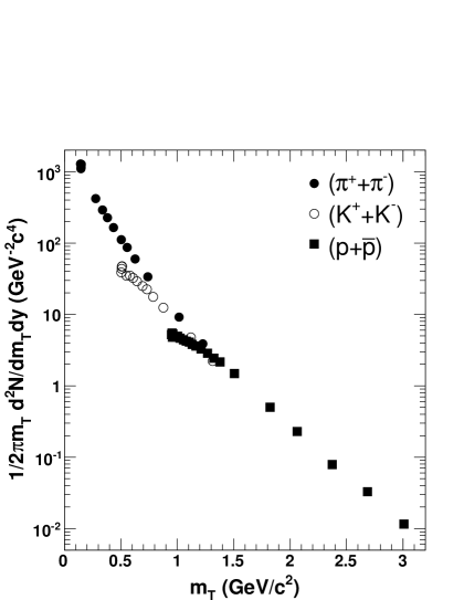
Figure 8: Transverse mass spectra of pions, kaons and protons in Au+Au collisions at $\sqrt{s_{{}_{NN}}}$=62.4 GeV energy. Particle and antiparticle yields are added to accommodate all three identification methods. Statistical errors are small compared to the symbol size.

It was shown earlier Veres et al. (2004) that the transverse mass ($m_{T}=\sqrt{m^{2}+p_{T}^{2}}$) spectra of the various hadron species in d+Au collisions at $\sqrt{s_{{}_{NN}}}$=200 GeV energy satisfy a scaling law within the experimental errors: they differ only by an $m_{T}$-independent scale factor. However, the scaling was shown to be violated in Au+Au collisions at the same collision energy Back et al. (2004d); Adler et al. (2004a). Figure 8 shows that the scaling violation is similar at $\sqrt{s_{{}_{NN}}}$=62.4 GeV in Au+Au collisions. Another important observation is that in Au+Au collisions the invariant yields for the three species seem to approximately converge for the $m_{T}$ region from 1 to 1.5 GeV/$c^{2}$, while in d+Au collisions at 200 GeV the kaon yield is suppressed with respect to the pion and proton yield by about a factor of two in the same $m_{T}$ range Veres et al. (2004).

Since the pion spectrum falls faster with transverse momentum than the proton spectrum (see Fig. 6), proton yields dominate over mesons at high $p_{T}$. This phenomenon may carry an important physics message about the relevant degrees of freedom in the radially expanding medium created by heavy-ion collisions. A similar observation was made previously at 200 GeV collision energy Adler et al. (2004a), where antiprotons were also found to dominate over negatively-charged mesons.

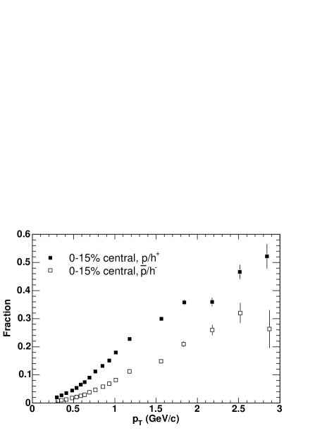
Figure 9: Fraction of protons among all positive hadrons, and antiprotons among all negative hadrons in Au+Au collisions at $\sqrt{s_{{}_{NN}}}$=62.4 GeV.

In order to study baryon dominance over mesons at high $p_{T}$, the fraction of protons among all positive hadrons ($p/h^{+}$) and the fraction of antiprotons among all negative hadrons ($\overline{p}/h^{-}$) is plotted in Fig. 9, for central Au+Au collisions at 62.4 GeV. This particular ratio was chosen because it can be measured up to 3 GeV/c transverse momentum (by taking the $h^{+}$ yield as the sum of $p$, $\pi^{+}$ and $K^{+}$ yields, etc.), while the measurable $p_{T}$ range of the $p/\pi^{+}$ and $\overline{p}/\pi^{-}$ ratios extends only up to 1.4 GeV/c.

The $p/h^{+}$ ratio reaches 0.5 above $p_{T}$=2.5 GeV/c, which means that the proton yield becomes comparable to the sum of pion and kaon yields: $Y_{p}\approx Y_{\pi^{+}}+Y_{K^{+}}$. The $\overline{p}/h^{-}$ ratio reaches 1/3 at around the same $p_{T}$ value, which means that either $Y_{\overline{p}}\geq Y_{\pi^{-}}$ or $Y_{\overline{p}}\geq Y_{K^{-}}$ becomes true, depending on whether the $K^{-}/\pi^{-}$ ratio is above or below unity (we were not able to measure this above $p_{T}$=1.4 GeV/c). One can conclude that baryons become the dominant particle species at about 2.5$-$3.0 GeV/c transverse momentum in central Au+Au collisions at 62.4 GeV energy.

Fig. 10 illustrates the evolution of this baryon dominance with collision energy. For central heavy-ion (Au+Au or Pb+Pb) collisions at AGS, SPS and RHIC energies, we study the $p_{T}$ value at which the invariant yields of protons and positive pions at mid-rapidity become equal. Data (fraction of most central events) are taken from the experiments: E802 Ahle et al. (1998) (4%), NA44 Bearden et al. (2002) (3.7%), NA49 Anticic et al. (2004) (5%), PHENIX Adler et al. (2004a); Adcox et al. (2004) (5%) and PHOBOS (15%). Although the pion spectrum from the present analysis does not reach above 1.4 GeV/c transverse momentum, the meson yield ($K+\pi$) can be measured up to 3 GeV/c. By allowing the extrapolation of the $K^{+}/\pi^{+}$ ratio to 2 GeV to change within reasonable limits, the location of the ‘crossing point’ can still be estimated with a meaningful systematic error. A remarkably smooth collision energy dependence of the ‘crossing’ $p_{T}$ value is observed. At low energies, the abundance of produced pions is naturally low compared to high collision energies, while baryon number conservation ensures that a significant fraction of the large number of initial state protons are found in the final state, thus the invariant yields of protons and positive pions become comparable already at low $p_{T}$. With increasing energy, this $p_{T}$ value grows, mainly due to the approximately logarithmically increasing number of produced pions.

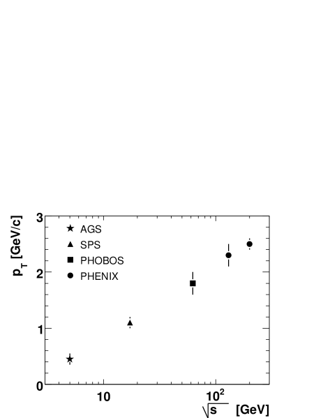
Figure 10: The $p_{T}$ value where the $\pi^{+}$ and proton invariant yields become equal in central Au+Au (Pb+Pb) collisions, as a function of $\sqrt{s_{{}_{NN}}}$. All data have been corrected for feed-down from weak decays. See text for references.

The dominance of the baryon yield is perhaps more interesting for antiparticles: antiprotons and negative pions, since all antiprotons are newly produced in the collision. Because of the strongly energy dependent production cross section of antiprotons, for the antiproton yield and the $\pi^{-}$ yield to be comparable, the highest RHIC collision energies are needed. This was observed for the first time in Au+Au collisions at $\sqrt{s_{{}_{NN}}}=130-200$ GeV Adcox et al. (2002a).

It is well known that the antiproton to proton ratio at midrapidity in Au+Au (Pb+Pb) collisions increases from a very small value to almost unity within the collision energy range plotted in Fig. 10. If one makes the simple assumption that part of the protons are transported from beam rapidities to midrapidity while other protons are pair produced (in approximately the same amount as the antiprotons), this ratio is the fraction of newly produced protons among all protons. At low energies, almost all midrapidity protons are transported from beam rapidities, while at the highest RHIC energy almost all protons are pair produced according to the above simple picture. Therefore, the fact that the proton and $\pi^{+}$ yields become comparable to each other at high $p_{T}$ also has implications on the baryon/meson differences of particle production at midrapidity. In jet fragmentation, which should be an important mechanism at high $p_{T}$, the expectation is to have a small baryon/meson ratio, as observed in elementary particle collisions Abreu et al. (2000). However, if a quark recombination process is dominant in the creation of baryons and mesons at midrapidity, the observed high baryon/meson ratio at $p_{T}$ of a few GeV/c is expected Hwa and Yang (2003).

It is worthwhile to discuss the baryon production and baryon transport features in connection with the above observations. The proton and antiproton invariant yields were integrated over $p_{T}$ at midrapidity, and subtracted to evaluate the net proton (defined as $p-\overline{p}$) rapidity density ($dN/dy$). The proton, antiproton and net proton integrated yields for all centrality bins are given in Table 2; the net proton yields are plotted in Fig. 11 as a function of the number of participant nucleons in the collision. For comparison, data measured by the PHENIX experiment at 200 GeV Adler et al. (2004a) are also shown, where the experimental errors on the proton and antiproton spectra are assumed to be completely correlated. Thus, the errors assigned to the net proton yields are lower limits. At both energies, the net proton density at midrapidity appears to be closely proportional to the number of participant nucleons. That proportionality means that the number of protons transported to midrapidity per initial state participant does not depend on the average number of collisions a participant suffers in the collision (which is strongly centrality dependent, changing between 2.91 and 4.65 for the 62.4 GeV data, and between 3.23 and 6.07 for the 200 GeV data plotted in Fig. 11).

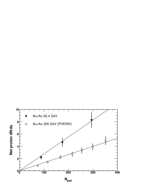
Figure 11: Net proton ($p-\overline{p}$) yield at midrapidity, as a function of the number of participant nucleons in the collision. Filled symbols are Au+Au collisions at 62.4 GeV energy from the present analysis, open symbols are Au+Au collisions at 200 GeV from PHENIX Adler et al. (2004a). In the latter case, the experimental errors on the proton and antiproton spectra were assumed to be completely correlated. The proportionality lines are only to guide the eye.

The $\overline{p}/p$ ratios in heavy ion collisions measured extensively by other experiments (e.g. Adler et al. (2004a) and Bearden et al. (2003) at 200 GeV and Adler et al. (2001) at 130 GeV) are approximately centrality-independent, and also approximately $p_{T}$-independent below 4-5 GeV/c transverse momentum. This means that the midrapidity proton and antiproton yields (and not only their difference) are approximately proportional to the number of participants.

IX Summary

The first identified hadron transverse momentum spectra from the Au+Au run at 62.4 GeV collision energy at RHIC were presented. This is also the first identified transverse momentum spectra analysis using the PHOBOS silicon Spectrometer and the first analysis using the Time of Flight detector. The very low $p_{T}$ data points are unique at RHIC. The identified particle spectra measured at 62.4 GeV also bridge a significant gap in collision energy between heavy ion collision data taken at the highest SPS energy and the high RHIC energies.

Centrality	$\frac{dN}{dy}$($p$)	$\frac{dN}{dy}$($\bar{p}$)	$\frac{dN}{dy}$($p-\bar{p}$)
0–15 %	$13.4\pm 1.9$	$5.1\pm 0.7$	$8.3\pm 1.3$
15–35 %	$7.7\pm 1.1$	$3.0\pm 0.4$	$4.6\pm 0.7$
35–50 %	$3.8\pm 0.5$	$1.6\pm 0.2$	$2.2\pm 0.3$

Table 2: Proton, antiproton and net proton ($p-\bar{p}$) integrated yields. The errors quoted are systematic, statistical errors are negligible. Correlations in the systematic errors for protons and antiprotons are included in the systematic error on the net proton yield.

Invariant cross sections of protons, antiprotons, pions and kaons in three centrality bins were presented. No significant enhancement of pions was found compared to a simple blast-wave parametrization at very low $p_{T}$, and the transverse momentum spectra are consistent with radial expansion down to very low $p_{T}$.

Remarkably, at about 2.5$-$3 GeV/c transverse momentum, the proton and antiproton yields exceed the yield of at least one of the meson species. The energy dependence of this baryon dominance was studied in detail. It was shown that the transverse momentum value where the $p/\pi^{+}$ ratio exceeds unity in central Au+Au (Pb+Pb) collisions is a very smooth function of the collision energy. The net baryon yield at midrapidity was, surprisingly, found to be closely proportional to the number of participant nucleons in the collision.

Appendix A Event Selection and Centrality

Determining the centrality of heavy ion collisions is important for event characterization. The centers of the ions travel along parallel lines before collision, displaced by $b$, called the impact parameter. The number of nucleons ‘participating’ (colliding at least with one other nucleon) in the collision, $\rm N_{\rm part}$, and the number of binary collisions between nucleon pairs, $\rm N_{\rm coll}$, can be connected to the impact parameter, using a simple geometrical model calculation.

None of these three quantities can be measured directly, but $\rm N_{\rm part}$ and $\rm N_{\rm coll}$ can be estimated from measured quantities. In PHOBOS, charged particle multiplicities in various pseudorapidity ($\eta$) regions are used to estimate centrality Back et al. (2005c). These $\rm N_{\rm part}$ and $\rm N_{\rm coll}$ centrality measures make it possible to study scaling of the hadron yields in peripheral and central heavy ion collisions, compared to elementary (p+p) collisions. The expectation is, that the number of ‘hard’ parton scatterings with large momentum transfer and small cross section should be proportional to $\rm N_{\rm coll}$. However, it was observed that the total number of charged particles as well as the hadron yields at low and even high $p_{T}$ is (approximately) proportional to $\rm N_{\rm part}$. It is important to study whether these observations hold for various hadron species separately.

The initial event selection used the time difference of the Paddle and Zero Degree Calorimeter signals, which were required to be less than 4 ns, to exclude beam-gas interactions. For very central events with few spectator neutrons but high Paddle signals, a hit in the ZDCs was not required. Separate logic filtered out events happening shortly after or before another collision, to avoid pile-up.

Since the geometrical acceptance of the Spectrometer strongly depends on the vertex position in the beam direction, an optimal vertex range was selected using the difference of the time signals from the two T0 detectors online, and a narrower, 20 cm wide vertex region was selected later offline, based on the precise vertex reconstruction using the silicon detectors.

The efficiency of the above trigger and selection was measured by comparison to a minimum bias type trigger, which required only a single hit in both Paddle detectors. Since the minimum bias trigger was only $91\pm 2\%$ efficient, a full Monte Carlo simulation accounted for the loss of the most peripheral events. After the efficiency determination, the data with the restrictive trigger could be sorted into bins according to percentage fractions of the total inelastic cross section, where the experimental variable measuring centrality was chosen to be the total energy deposited in the Paddles.

In the present analysis, the most central 50% of the total cross section was used, where the triggering and vertex finding was still fully efficient, and divided into the three centrality classes: the 15% most central events, and two more bins between 15–30% and 30–50%.

Comprehensive Monte Carlo simulations of the Paddle signals, including Glauber model calculations of the collision geometry, allowed the estimation of the number of participating nucleons, $\langle{\rm N_{part}}\rangle$, for each total cross section bin. The systematic uncertainty of ${\rm N_{part}}$ was estimated with MC simulations taking into account possible errors in the overall trigger efficiency and by using different types of event generators.

The average number of binary nucleon-nucleon collisions, $\langle\rm{N_{coll}}\rangle$, was found from a parametrization of the results of a Glauber calculation Back et al. (2005c): $\langle\rm{N_{coll}}\rangle$= 0.296$\langle\rm{N_{part}}\rangle^{1.376}$. In this way, the $\rm{N_{part}}$ determination, which is relatively insensitive to the parameters of the MC event generators, and the relation between $\rm{N_{coll}}$ and $\rm{N_{part}}$, which depends strongly on cross sections used, are conveniently decoupled.

Appendix B Track Reconstruction

Signals in individual Spectrometer pixels are first clustered to obtain ‘hits’. The thresholds are determined in terms of the energy deposited by a Minimum Ionising Particle (MIP), which is found to be 80 keV for the 300 $\mu$m-thick PHOBOS silicon sensors. Any pixel with a signal above 0.15 MIP is considered a candidate for merging. Adjacent pads in the horizontal direction can be merged if they are above this threshold, up to a limit of 8 pads per hit candidate. A set of merged pads must sum to over 0.5 MIP before being declared a ‘hit’. There is no vertical merging of pixels.

Straight-line tracks are reconstructed in the low-field region of the Spectrometer (in the layers closest to the beam pipe) using a road-following algorithm. Track candidates are required to have hits from at least five of the six inner layers and to point back to the independently-determined event vertex.

Combined with the event vertex location, a pair of hits from consecutive layers in the high field region can be mapped to the total momentum $p$ and polar angle $\theta$ of the track which would have produced those hits. Track reconstruction therefore looks for clusters of hit pairs in $(p,\theta)$ space that correspond to a trajectory which traverses all layers.

Curved and straight track pieces are joined by requiring consistency in their $\theta$ and $\phi$ angles and in the average energy deposited per hit.

The track trajectory is found by propagating the momentum vector through the PHOBOS magnetic field using a Runge-Kutta algorithm and detailed field map. At this stage, no effects such as multiple scattering or energy loss are included. This determines the trajectory relative to which hit residuals are calculated.

The track momentum is determined by a $\chi^{2}$ fit to the reconstructed hit pattern. The error for each hit position is influenced by deflection of the charged particle due to multiple scattering and pixelisation of the silicon sensors. Multiple scattering also introduces a correlation between the errors on different hits, because a deflection in one layer tends to produce systematic offsets in the hit-residuals for subsequent layers.

The PHOBOS tracking package uses a complete covariance matrix to account for these correlations. Covariance matrices are pre-generated using Monte Carlo simulation of pions passing through the Spectrometer, including the effects of multiple scattering and energy loss due to interaction with the detector material.

The actual minimisation procedure to find the best trajectory uses a standard ‘downhill simplex’ technique Press et al. (2002). This multi-dimensional minimisation method does not require knowledge of the derivatives of the function being minimised. That is important because the non-uniform magnetic field means that there is no analytic form for the particle trajectory and, therefore, accurate derivatives cannot easily be computed. The procedure not only finds the best-fit trajectory but also assigns a goodness-of-fit value. This variable is found to be a powerful tool for rejecting tracks resulting from incorrect hit associations. Distinct tracks are not allowed to share more than two hits. If a pair of candidates share more than two hits, the one with the lower fit probability is discarded.

Since the track reconstruction procedure assumes pions, heavier particles like kaons and protons will deposit more energy than the template track and hence be assigned a reconstructed momentum that is systematically too small. Monte Carlo simulations are used to obtain momentum correction factors for tracks which are identified to be kaons or protons.

The track reconstruction efficiency is about 80%. The momentum resolution achieved by this tracking package is about 1% for total momentum $p\approx$1 GeV/c and rises linearly with $p$, but is still less than 5% for $p$=8 GeV/c.

For particle identification by Time-of-Flight, the reconstructed Spectrometer tracks are extrapolated towards the TOF detector. This extrapolation uses the same Runge-Kutta algorithm as the track reconstruction, in combination with a detailed map of the (small but non-zero) magnetic field in the region between the Spectrometer and the TOF. It is found that a better match is obtained when the track extrapolation uses the momentum value obtained by fitting without covariance matrices – this technique gives a better fit to the track momentum as it exits the Spectrometer. However, the original momentum value is retained and is still the value used for physics.

Signals in the TOF sensors are checked for good timing characteristics and sufficient deposited energy to indicate a true charged-particle detection. The timing and pulse-height information from the photomultiplier tubes at both ends of the sensors are required to be consistent. TOF hits are then matched to the best extrapolated Spectrometer track. A residual (minimum distance of TOF hit from extrapolated track trajectory) of less than 4 cm is required for matching. Over a distance of more than 4 m from the last Spectrometer layer to the TOF wall, tracks are matched to TOF hits with a resolution of 1.5 cm (3.5 cm FWHM).

Appendix C Particle Identification in the Spectrometer

C.1 Very low momentum particles

The determination of particle mass at very low transverse momenta (0.03–0.05 GeV/c for pions, 0.09–0.13 GeV/c for kaons and 0.14–0.21 GeV/c for protons) was based on detailed GEANT simulations of the measured energy depositions in the first detector layers. The required smallest specific energy loss ($dE/dx$) was six times that of a minimum ionizing particle (MIP). Consistency between energy deposited in the different layers, and consistency between the mean measured $dE/dx$ and the expected specific energy loss from the simulations was used to distinguish between pions, protons and kaons. Additional cuts on the deviations of the candidate track from a straight line trajectory (allowing for mass and momentum dependent multiple scattering) were used to reject fake tracks. The first five layers of the Spectrometer are located in a magnetic field smaller than 0.3 T, which is insufficient to cleanly separate positive and negative particles. Therefore at very low momenta, only the sum of positive and negative particle yields are presented: ($\pi^{+}+\pi^{-}$), (K⁺+K^-) and (p+$\overline{\rm p}$). More details about the low-$p_{T}$ analysis and corrections applied to these results can be found in the report on a similar measurement completed at $\sqrt{s_{{}_{NN}}}=$200 GeV Back et al. (2004d).

C.2 Particles with intermediate momenta

Identification based on the truncated mean value of the specific energy loss ($dE/dx$) in the silicon layers was applied to particles with high enough momentum to safely travel through the whole silicon Spectrometer system. The total momentum range for this PID method was 0.2–0.9 GeV/c for pions and kaons, and 0.3–1.4 GeV/c for protons and antiprotons. In the measured momentum range the $dE/dx\propto 1/v^{2}$ relation holds, where $v$ is the velocity. Thus, particles with the same total momentum lose different amounts of energy in the spectrometer layers (top panel of Fig. 2).

The particles can only be identified individually at low momentum, therefore a fit method was applied which significantly extends the momentum reach by counting abundances of the various species in a statistical sense. The particles were sorted into total momentum bins and fits to the specific energy loss ($dE/dx$) histograms (inset in Fig. 2) were performed. Yields of pions and kaons are quoted only below 0.6 GeV/c transverse momentum, where they produce sufficiently different amount of ionization. The fits no longer work below 0.2 GeV/c total momentum because of low statistics caused by low tracking efficiency and acceptance, and both the efficiency and momentum corrections become large and poorly known.

At first, $dE/dx$ (truncated mean of the path length-corrected specific ionization values) of each track in a given total momentum ($p$) bin are collected. At the same time, the $p$ and transverse momentum ($p_{T}$) distributions of these tracks are also collected.

A Gaussian fit to the pion $dE/dx$ peak is performed in the momentum bin of $p$ = 0.55$\pm$0.05 GeV/c, where the kaons and pions are well separated, to measure the $dE/dx$ resolution. The width is found to be about 0.07 MIP, but this overestimates the resolution because the momentum spread within this bin widens the $dE/dx$ distribution.

For the theoretical $dE/dx$ function, a form of the Bethe-Bloch formula was used where all of the constants in it were collapsed into two variables. One ($E_{0}$) is an overall constant, and the other ($b$=20) characterizes the relative strength of the logarithmic rise:

$$dE/dx=E_{0}\beta^{-2}(b+2\ln\gamma-\beta^{2})$$ (2)

For each $p$ bin, the convolution of the theoretical $dE/dx$ function (between the bin edges) and the resolution function gives the line shape for each species. More precisely, a sum of a Gaussian and a half Gaussian both with the mean given by Equation 2 but different width and amplitude was used to create a more realistic lineshape, to account for the natural remnant of the Landau-tail of the $dE/dx$ (truncated mean) distribution. The ‘main’ Gaussian accounts for 90% of the total lineshape integral; the other 10% is accounted for by the half Gaussian with twice the width on the positive side of the distribution. The $dE/dx$ resolution used is momentum dependent; $\sigma(dE/dx)\propto(dE/dx)^{\alpha}$. The best lineshape fit was found using $\alpha=0.9$. This slightly non-Gaussian lineshape gives a good description of the experimental $dE/dx$ histograms (see Fig. 2).

After building the lineshapes, the only free parameters are the amplitudes (yields) of the three particle species. A three-parameter $\chi^{2}$ fit, using the proper weights (the square-root of the bin counts) gives the errors of the yields correctly, including the errors caused by overlaps (correlations between yields). A second fit, where all the weights are set to unity (independent of bin content) gives a more precise estimate of the integral of the line shapes by suppressing the importance of tails and outliers of the distribution. Thus, the second fit was used to obtain the yields while the first one was used for the statistical error.

This method gives a reliable fit when the particle peaks are separate. Above 1.4 GeV/c transverse momentum, the pion and kaon peaks merge and separate fits to kaons and pions are no longer possible. However, a lineshape for the meson peak is still needed to be able to fit the proton (and meson) yield. Here, a certain $K/\pi$ ratio (as a function of $p_{T}$) had to be assumed to build the meson lineshape. The $K/\pi$ ratio was measured as a function of $p_{T}$ below 1.4 GeV/c, where the particles are still separated, and extrapolated to higher $p_{T}$ values. Any particular extrapolation gets less justified with increasing momentum, but at the same time, the assumed $K/\pi$ ratio affects the line shape description less, since only a very small difference remains between the mean $dE/dx$ value expected for kaons and pions. Thus, the systematic error on the proton yield caused by the uncertainty of the meson line shape depends only weakly on $p_{T}$, and was found to be a few percent.

Appendix D Corrections

The corrections applied to the invariant particle yields are discussed in the following sections.

D.1 Geometrical Acceptance and Tracking Efficiency

The most important corrections to the raw particle yields are to account for the geometrical acceptance of the detector and the momentum dependence of the track-reconstruction efficiency. These two corrections are combined in a Monte Carlo study of single particles passing through a GEANT simulation of the PHOBOS detector and the full track reconstruction package. This gives the probability, as a function of transverse momentum, that an individual particle will be properly reconstructed. These functions, obtained for each particle species over the whole phase space, are used to correct the raw distributions.

D.2 Occupancy Correction in the Spectrometer

The track-reconstruction efficiency is to a small extent dependent on the occupancy of the Spectrometer. This effect is studied by embedding and reconstructing individual Monte Carlo tracks in real data events. For central Au+Au collisions at 62.4 GeV, the difference relative to the single track case was found to be $\sim$10%, independent of momentum.

D.3 Ghost Correction

After accounting for the efficiency of the track-reconstruction procedure, we must also account for its purity, since it is possible that it will produce spurious tracks, called ‘ghosts.’ Ghost contributions depend on both the track momentum and the hit density and are determined by reconstructing Monte Carlo events, where the tracking output can be compared to the known input tracks. The ghost fraction is found to range from roughly 2% for the most peripheral events used in this analysis to 5% for the most central, with an approximately exponential dependence on transverse momentum. No species dependence was found.

D.4 Momentum Resolution Correction

The momentum resolution of the Spectrometer in our momentum range (up to $p_{T}=3$ GeV/c) is a few percent. The correction of the invariant yields for this momentum resolution depends on the steepness of the momentum distributions, and can be estimated to be 2-3% at $p_{T}=3$ GeV/c, where it reaches its maximum. However, instead of an explicit momentum resolution correction, an implicit one was used in the present analysis. The efficiency of the detector system was estimated using Monte Carlo techniques, where single tracks weighted by the closely exponential transverse momentum distribution were generated, and reconstructed (with the momentum resolution entering the procedure at this step). The reconstructed MC track sample was analyzed the same way as the data and compared to the originally assumed exponential $p_{T}$ distribution. Therefore the momentum resolution correction is taken care of by the efficiency correction in an implicit way.

D.5 Feed-down Correction

Contributions to the measured transvserse momentum spectra from particles which are products of weakly-decaying resonance states are detector-dependent, and therefore should be removed.

D.5.1 Proton Feed-down

For a reconstructed proton we need to know the probability that it is a primary particle and not the product of a weak decay. To obtain this, one needs to know the relative efficiency of reconstructing primary protons versus those which are products of weak decays, and also know the yield of primary protons relative to particles which can produce protons by weak decay.

The major feed-down contribution to the proton yields comes from the $\Lambda$ decay: $\Lambda\rightarrow p+\pi^{-}$. This process has a branching ratio of 63.9% and a lifetime expressed as $c\tau=7.9$ cm; the daughter particles have a momentum of 101 MeV/c in the center of mass frame.

The $\Lambda$, being neutral, leaves no trace as it passes through the silicon detectors. The PHOBOS tracking procedures are such that the daughter proton will only be reconstructed if the decay happens before the first spectrometer layer. As this layer is only roughly 10 cm from the nominal interaction point, the PHOBOS experiment has sensitivity to distinguish between primary and feed-down protons.

The GEANT Monte Carlo package was used to simulate single $\Lambda$ decays in the PHOBOS spectrometer. $\Lambda$s were generated with realistic transverse momentum distributions, and the efficiency of reconstructing the daughter proton at a given momentum can then be compared to the efficiency for primary proton reconstruction at the same momentum. This result can then be scaled according to the $\Lambda/p$ ratio to determine, as a function of transverse momentum, the fraction of observed protons which are expected to actually originate from $\Lambda$ decays. This method was tested on Monte Carlo events produced by the HIJING event generator. In this case, the $\Lambda/p$ ratio was known, and this method was able to correctly describe the contribution from feed-down protons.

The PHENIX collaboration has measured $\Lambda/p=0.89\pm 0.07$ in Au+Au collisions at $\sqrt{s_{{}_{NN}}}=130$ GeV Adcox et al. (2002c). The value at 62.4 GeV is not yet known, which leads to an uncertainty in the feed-down correction. Studies were performed for a variety of different values of the ratio in the range $0.7\leq\Lambda/p\leq 1.1$.

Feed-down protons can also originate from the decay $\Sigma^{+}\rightarrow p+\pi^{0}$, which has a branching ratio of 51.6% and $c\tau=2.4$ cm. The $\Sigma/p$ ratio has not been measured for Au+Au collisions at RHIC. The HIJING event generator predicts $\Sigma/p\approx 0.3$, and measurements from p+p collisions at similar energies have found a value of around 0.5. Monte Carlo studies of single $\Sigma$ decays in the PHOBOS detector were performed using the same techniques as for $\Lambda$s, taking the ratio $\Sigma/p$ in the range $0.1\leq\Sigma/p\leq 0.9$. For the final correction the $\Lambda/p=0.9$ and $\Sigma/p=0.3$ ratios were used, as discussed in the following paragraphs.

The distance of closest approach of a reconstructed track to the event vertex (DCA) is a quantity which has sensitivity for distinguishing between primary particles and those which did not originate from the event vertex. This is particularly useful for the study of feed-down particles. From the Monte Carlo simulations described above, the DCA distributions for primary and feed-down protons were obtained. In the case of primaries, the DCA distribution is narrow, reflecting the fact that these particles really did originate at the event vertex. The distribution for feed-down particles has a tail which extends to much higher values of DCA. The cut on DCA $<0.35$ cm used as part of track selection was found to remove $\sim 25$% of the feed-down protons but only $\ll 1$% of the primaries.

The simulated primary and feed-down DCA distributions were combined to reproduce the observed distribution for data protons. It was found that a feed-down contribution in the range of 25-30% gave the best consistency, and that less than 20% or greater than 35% seemed to be inconsistent with the data. The left panel of Figure 12 illustrates the proton DCA distribution for the identified protons in the data (dots), compared to simulated primary and weak decay daughter (secondary) protons, where the contribution of secondaries is set to 25%. On the right panel, the identified kaon DCA distribution is plotted, together with the simulated primary kaon DCA distribution. The agreement confirms that there are no secondary kaons originating from weak decays visible in the data.

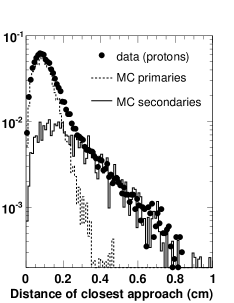
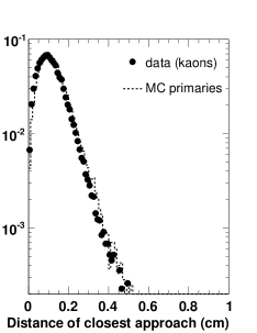
Figure 12: Distribution of the distance of closest approach between the track and the event vertex for protons (left panel) and for kaons (right panel). The dots are identified protons and kaons from the data, the histograms are Monte Carlo-simulated primary protons and kaons (dashed lines) and secondaries (weak decay daughters, solid lines) assuming 25% secondary contribution below 0.35 cm for the protons.

The final feed-down correction for protons is chosen to be the sum of the simulated contributions from $\Lambda$ and $\Sigma$ decays, assuming $\Lambda/p=0.9$ and $\Sigma/p=0.3$. This gives a correction which is consistent with the data-driven feed-down estimates from the DCA distributions. The systematic uncertainty on this correction comes from plausible variations in the $\Lambda/p$ and $\Sigma/p$ ratios (which have not yet been measured for $62.4$ GeV Au+Au collisions) and are also consistent with the bounds obtained from the DCA analysis.

The function used for the fraction of observed protons which are feed-down products is:

$$f(p_{T})=0.39e^{-0.57p_{T}}+(0.22p_{T}-0.16)e^{-5p_{T}^{2}}$$ (3)

with upper and lower bounds defined by $(1.22+0.1p_{T})f(p_{T})$ and $(0.78-0.1p_{T})f(p_{T})$ respectively.

D.5.2 Antiproton Feed-down

We determine the antiproton feed-down correction in relation to that for protons by making the reasonable assumption that antiproton feed-down is dominated by $\bar{\Lambda}$ decays and therefore the main difference between proton and antiproton feed-down comes from differences in the $\bar{\Lambda}/\bar{p}$ and $\Lambda/p$ ratios.

The value of these ratios in Au+Au collisions at $\sqrt{s_{{}_{NN}}}=$130 GeV has been measured Adcox et al. (2002c) to be:

$$\frac{\Lambda}{p}=0.89\pm 0.07\mbox{(stat)}$$

$$\frac{\bar{\Lambda}}{\bar{p}}=0.95\pm 0.09\mbox{(stat)}$$

By considering the quark content of these states, one can postulate that they should be related by:

$$\frac{\bar{\Lambda}}{\bar{p}}=\frac{\Lambda}{p}\times\frac{K^{+}}{K^{-}}$$ (4)

This relationship was found to hold true for 130 GeV Au+Au collisions, where the kaon ratio was measured Back et al. (2001) to be: $K^{-}/K^{+}=0.91\pm 0.07\mbox{(stat)}\pm 0.06\mbox{(sys)}$.

We assume it holds at 62.4 GeV also, where we have made preliminary measurements of $K^{-}/K^{+}\approx 0.85$. Thus we take the antiproton feed-down correction to be roughly $1.0/0.85=1.18$ times the correction for protons.

D.5.3 Feed-down to Kaons and Pions

There are no weak processes which produce kaons as the final state, thus there is no feed-down correction for the kaon yields. This expectation from theoretical grounds is verified by the observed DCA distribution for reconstructed kaons. The data agree well with the distribution for primary kaons obtained from Monte Carlo simulations, with no indication of a tail that would correspond to feed-down contributions.

The DCA distribution for pions from data was also studied and compared to that for simulated primary pions. The feed-down contribution to the pion yields after applying the cut of DCA $<0.35$ cm was estimated to be less than 1% and was therefore neglected, but this was included as a 1% contribution to the overall systematic uncertainty on the pion spectra.

D.6 Secondaries

Secondary particles are here defined as those which did not originate directly from the heavy-ion collision and are not the product of weak decays. The main sources of secondaries are interactions of primary particles with the beryllium beampipe and other detector material.

Production of secondary particles is studied using a GEANT simulation of the PHOBOS detector, with the HIJING event generator as the source of primary particles. On average, secondary particles tend to be produced with very low momentum. This means that they are unlikely to be detected in our Spectrometer because they tend to bend out of the acceptance and also suffer more multiple scatterings, making their hit pattern less likely to be reconstructed as a track.

Secondaries were only found to contribute significantly to the total proton yield for $p_{T}<200$ MeV/c. As this analysis does not extend this low in transverse momentum, the secondary correction to our measured proton yield is actually less than 1%. We therefore choose to neglect this correction, but make an additional contribution of 1% to the systematic uncertainty of the spectra. The secondary contribution to kaon and pion yields was found to be negligible.

D.7 Dead Channels in the Spectrometer and in the TOF

Some of the electronics channels in the silicon Spectrometer do not produce a signal when a charged particle passes through the silicon pad attached to it, and some other channels are called ‘hot’ since they produce a signal even without particles crossing. The fraction of these faulty channels is on the percent level. They are identified by inspecting the energy deposit ($dE$) distributions channel by channel, where the above failures of operation are found. The set of these faulty channels are excluded from the analysis.

Technically, the full data sample is reconstructed by using all the channels, and a separate dead channel correction is applied. The correction is obtained by reconstructing part of the data, as well as the Monte Carlo track sample again with the dead/hot channels excluded. Since the exclusion of channels decreases the number of found tracks in both the data and the Monte Carlo samples (where the latter is used to quantify the geometrical acceptance and efficiency), the dead channel correction is applied as the ratio of the change of the track yields in the two cases.

Another type of dead channel correction is performed on the number of tracks detected by the Time of Flight wall for the part of data that uses the TOF information. Four out of the 120 channels of the TOF wall are dead, and there are no hot channels. By comparing the hit frequency distribution of the 116 live channels (which is a linear function of the channel number to a good approximation) to the position of the missing channels, the reduction of measured yield for the entire wall caused by the missing channels is estimated to be 3%, and that correction is applied to the data.

References

- Back et al. (2005a) B. B. Back et al. (PHOBOS), Phys. Rev. Lett. 94, 082304 (2005a), eprint nucl-ex/0405003.
- Adler et al. (2004a) S. S. Adler et al. (PHENIX), Phys. Rev. C69, 034909 (2004a), eprint nucl-ex/0307022.
- Adcox et al. (2002a) K. Adcox et al. (PHENIX), Phys. Rev. Lett. 88, 242301 (2002a), eprint nucl-ex/0112006.
- Adcox et al. (2004) K. Adcox et al. (PHENIX), Phys. Rev. C69, 024904 (2004), eprint nucl-ex/0307010.
- Adcox et al. (2002b) K. Adcox et al. (PHENIX), Phys. Rev. Lett. 88, 022301 (2002b), eprint nucl-ex/0109003.
- Adcox et al. (2003) K. Adcox et al. (PHENIX), Phys. Lett. B561, 82 (2003), eprint nucl-ex/0207009.
- Adler et al. (2004b) S. S. Adler et al. (PHENIX), Phys. Rev. C69, 034910 (2004b), eprint nucl-ex/0308006.
- Adler et al. (2002) C. Adler et al. (STAR), Phys. Rev. Lett. 89, 202301 (2002), eprint nucl-ex/0206011.
- Adams et al. (2003) J. Adams et al. (STAR), Phys. Rev. Lett. 91, 172302 (2003), eprint nucl-ex/0305015.
- Back et al. (2004a) B. B. Back et al. (PHOBOS), Phys. Lett. B578, 297 (2004a), eprint nucl-ex/0302015.
- Arsene et al. (2003) I. Arsene et al. (BRAHMS), Phys. Rev. Lett. 91, 072305 (2003), eprint nucl-ex/0307003.
- Gyulassy and Plumer (1990) M. Gyulassy and M. Plumer, Phys. Lett. B243, 432 (1990).
- Back et al. (2003a) B. B. Back et al. (PHOBOS), Nucl. Instr. Meth. A499, 603 (2003a).
- Bindel et al. (2001) R. Bindel, E. Garcia, A. Mignerey, and L. Remsberg, Nucl. Instr. Meth. A474, 38 (2001).
- Adler et al. (2003) C. Adler et al., Nucl. Instrum. Meth. A499, 433 (2003).
- Nouicer et al. (2001) R. Nouicer et al., Nucl. Instr. Meth. A461, 143 (2001).
- Back et al. (2004b) B. B. Back et al. (PHOBOS), Phys. Lett. B578, 297 (2004b), eprint nucl-ex/0302015.
- Back et al. (2003b) B. B. Back et al. (PHOBOS), Phys. Rev. Lett. 91, 072302 (2003b), eprint nucl-ex/0306025.
- Back et al. (2004c) B. B. Back et al. (PHOBOS), Phys. Rev. C70, 061901(R) (2004c), eprint nucl-ex/0406017.
- Back et al. (2004d) B. B. Back et al. (PHOBOS), Phys. Rev. C70, 051901(R) (2004d), eprint nucl-ex/0401006.
- Back et al. (2001) B. B. Back et al. (PHOBOS), Phys. Rev. Lett. 87, 102301 (2001), eprint hep-ex/0104032.
- Back et al. (2003c) B. B. Back et al. (PHOBOS), Phys. Rev. C 67, 021901(R) (2003c), eprint nucl-ex/0206012.
- Back et al. (2004e) B. B. Back et al. (PHOBOS), Phys. Rev. C 70, 011901(R) (2004e), eprint nucl-ex/0309013.
- Back et al. (2005b) B. B. Back et al. (PHOBOS), Phys. Rev. C 71, 021901(R) (2005b), eprint nucl-ex/0409003.
- Schnedermann et al. (1993) E. Schnedermann, J. Sollfrank, and U. Heinz, Phys. Rev. C48, 2462 (1993), eprint nucl-th/9307020.
- Veres et al. (2004) G. I. Veres et al. (PHOBOS), J. Phys. G30, S1143 (2004).
- Ahle et al. (1998) L. Ahle et al. (E802), Phys. Rev. C57, 466 (1998).
- Bearden et al. (2002) I. G. Bearden et al. (NA44), Phys. Rev. C66, 044907 (2002), eprint nucl-ex/0202019.
- Anticic et al. (2004) T. Anticic et al. (NA49), Phys. Rev. C69, 024902 (2004).
- Abreu et al. (2000) P. Abreu et al. (DELPHI), Eur. Phys. J. C17, 207 (2000), eprint hep-ex/0106063.
- Hwa and Yang (2003) R. C. Hwa and C. B. Yang, Phys. Rev. C67, 034902 (2003), eprint nucl-th/0211010.
- Bearden et al. (2003) I. G. Bearden et al. (BRAHMS), Phys. Rev. Lett. 90, 102301 (2003).
- Adler et al. (2001) C. Adler et al. (STAR), Phys. Rev. Lett. 86, 4778 (2001), eprint nucl-ex/0104022.
- Back et al. (2005c) B. B. Back et al. (PHOBOS), Nucl. Phys. A757, 28 (2005c), eprint nucl-ex/0410022.
- Press et al. (2002) W. H. Press, S. A. Teukolsky, W. T. Vetterling, and B. P. Flannery, Numerical Recipes in C++: The Art of Scientific Computing (Cambridge University Press, 2002), 2nd ed.
- Adcox et al. (2002c) K. Adcox et al. (PHENIX), Phys. Rev. Lett. 89, 092302 (2002c), eprint nucl-ex/0204007.