Critical behavior of number-conserving cellular automata with nonlinear fundamental diagrams

Abstract

We investigate critical properties of a class of number-conserving cellular automata (CA) which can be interpreted as deterministic models of traffic flow with anticipatory driving. These rules are among the only known CA rules for which the shape of the fundamental diagram has been rigorously derived. In addition, their fundamental diagrams contain nonlinear segments, as opposed to majority of number-conserving CA which exhibit piecewise-linear diagrams. We found that the nature of singularities in the fundamental diagram of these rules is the same as for rules with piecewise-linear diagrams. The current converges toward its equilibrium value like $t^{-1/2}$, and the critical exponent $\beta$ is equal to $1$. This supports the conjecture of universal behavior at singularities in number-conserving rules. We discuss properties of phase transitions occurring at singularities as well as properties of the intermediate phase.

1 Introduction

Cellular automata (CA) can be viewed as cells in a regular lattice updated synchronously according to a local interaction rule, where the state of each cell is restricted to a finite set of allowed values. An interesting subclass of CA consists of rules possessing an additive invariant. The simplest of such invariants is the total number of sites in a particular state. CA with such invariant, often called “conservative CA” or “number-conserving CA”, can be viewed as a system of interacting and moving particles, where in the case of a binary rule, 1’s represent sites occupied by particles, and 0’s represent empty sites.

In a finite system, the flux or current of particles in equilibrium depends only on their density, which is invariant. The graph of the current as a function of density characterizes many features of the flow, and is therefore called the fundamental diagram. For a majority of conservative CA rules, fundamental diagrams are piecewise-linear, usually possessing one or more “sharp corners” or singularities. There exist a strong evidence of universal behavior at singularities, as reported in [1].

Conservative CA appear in various applications, and some special cases have been studied extensively. Rule 184, which is a discrete version of the totally asymmetric exclusion process, is an example of such special case [2, 3, 4, 5, 7, 8, 9, 10]. Although much is known about this particular rule, dynamics of other conservative rules exhibits many features which are not fully understood, and more general results are just starting to appear [11, 12, 13, 14, 15]. In particular, there exists no general result explaining the shape of fundamental diagrams for conservative Ca, although promising results have been obtained for some special cases by Kujala and Lukka [16], who studied a class of deterministic traffic rules introduced by [17]. Using their results, we will study numerically behavior of singularities for number-conserving rules with fundamental diagrams different that previously reported.

It should be emphasized at this point that all CA rules considered in this paper are strictly deterministic. Nevertheless, they are strongly related to stochastic CA models of road traffic flow, which have gained widespread attention in recent years [18, 19].

2 Number-conserving cellular automata

In what follows, we will assume that the dynamics takes place on one-dimensional lattice of length $L$ with periodic boundary conditions. Let $s_{i}(t)$ denote the state of the lattice site $i$ at time $t$, where $i\in\{0,1,\ldots,L-1\}$, $t\in\mathbbm{N}$. All operations on spatial indices $i$ are assumed to be modulo $L$. We will further assume that $s_{i}(t)\in\{0,1\}$, and we will say that the site $i$ is occupied (empty) at time $t$ if $s_{i}(t)=1$ ($s_{i}(t)=0$).

Let $l$ and $r$ be two integers such that $l\leq 0\leq r$, and let $n=r-l+1$. The set $\{s_{i+l}(t),s_{i+l+1}(t),\ldots,s_{i+r}(t)\}$ will be called the neighbourhood of the site $s_{i}(t)$. Let $f$ be a function $f:\{0,1\}^{n}\rightarrow\{0,1\}$, also called a local function The update rule for the cellular automaton is given by

$$s_{i}(t+1)=f(s_{i+l}(t),s_{i+l+1}(t),\ldots,s_{i+r}(t)).$$ (1)

The CA rule given by (1) will be called number conserving if

$$\sum_{i=0}^{L-1}f(x_{i+l},x_{i+l+1},\ldots,x_{i+r})=\sum_{i=0}^{L-1}x_{i}$$ (2)

for all $\{x_{0,}x_{1},\ldots,x_{L-1}\}\in\{0,1\}^{L}$. Note that the above condition simply states that the number of occupied sites is constant in time.

In [20], Hattori and Takesue demonstrated that CA rules are number-conserving if and only if a discrete version of a standard current conservation law $\partial\rho/\partial t=-\partial j/\partial x$ is satisfied. More precisely, CA rule $f$ is number-conserving if and only if for all $\{x_{1},x_{2},\ldots,x_{n}\}\in\{0,1\}^{n}$ it satisfies

$$f(x_{1},x_{2},\ldots,x_{n})-x_{-l+1}=J(x_{1},x_{2},\ldots,x_{n-1})-J(x_{2},x_{3},\ldots,x_{n}),$$ (3)

where

$$J(x_{1},x_{2},\ldots,x_{n-1})=-\sum_{k=1}^{n-1}f(\underbrace{0,0,\ldots,0}_{k},x_{1},x_{2},\ldots,x_{n-k})+\sum_{j=1}^{-l}x_{j}.$$ (4)

Applying this to all lattice sites we obtain

$$f(s_{i+l},\ldots,s_{i+r})-s_{i}=J(s_{i+l},\ldots,s_{i+r-1})-J(s_{i+l+1},\ldots,s_{i+r}),$$ (5)

where we dropped $t$ dependence for clarity.

The above equation can be interpreted in a similar way as a conservation law in a continuous, one dimensional physical system. In such system, let $\rho(x,t)$ denote the density of some material at point $x$ and time $t$, and let $j(x,t)$ be the current (flux) of this material at point $x$ and time $t$. A conservation law states that the rate of change of the total amount of material contained in a fixed domain is equal to the flux of that material across the surface of the domain. The differential form of this condition can be written as

$$\frac{\partial\rho}{\partial t}=-\frac{\partial j}{\partial x}.$$ (6)

Interpreting $s_{i}(t)$ as the density, the left hand side of (5) is simply the change of density in a single time step, so that (5) is an obvious discrete analog of the current conservation law (6) with $J$ playing the role of the current.

Let us now assume that the initial distribution $\mu$ is a Bernoulli distribution, i.e., at $t=0$, all sites $s_{i}(t)$ are independently occupied with probability $p$ or empty with probability $1-p$, where $p\in[0,1]$. Let us define

$$\rho(i,t)=E_{\mu}(s_{i}(t)).$$ (7)

Since the initial distribution is $i$-independent, we expect that $\rho(i,t)$ also does not depend on $i$, and we will therefore define $\rho(t)=\rho(i,t)$. Furthermore, for conservative CA, $\rho(t)$ is $t$-independent, so we define $\rho=\rho(t)$. For the aforementioned Bernoulli distribution we thus obtain $\rho=p$. We will refer to $\rho$ as the density of occupied sites. The expected value of the current $J(s_{i+l}(t),s_{i+l+1}(t),\ldots,s_{i+r-1}(t))$ will also be $i$-independent, so we can define the expected current as

$$j(\rho,t)=E_{\mu}\big{(}J(s_{i+l}(t),s_{i+l+1}(t),\ldots,s_{i+r-1}(t))\big{)}.$$ (8)

The graph of the equilibrium current $j(\rho,\infty)=\lim_{t\rightarrow\infty}j(\rho,t)$ versus the density $\rho$ is known as the fundamental diagram. It has been numerically demonstrated [21] that for conservative deterministic CA the fundamental diagram usually develops a singularity as $t\rightarrow\infty$, meaning that $j(\rho,\infty)$ is not everywhere differentiable function of $\rho$. A well-know example is CA rule 184, for which

$$s_{i}(t+1)=f\Big{(}s_{i-1}(t),s_{i}(t),s_{i+1}(t)\Big{)},$$ (9)

and $f$ is defined by

$$f(0,0,0)=0,\,f(0,0,1)=0,\,f(0,1,0)=0,$$

$$f(0,1,1)=1,\,f(1,0,0)=1,\,f(1,0,1)=1,$$

$$f(1,1,0)=0,\,f(1,1,1)=1.$$ (10)

The above definition can also be written in a form (5) as

$$s_{i}(t+1)=s_{i}(t)+J(s_{i-1}(t),s_{i}(t))-J(s_{i}(t),s_{i+1}(t)),$$ (11)

where $J(x_{1},x_{2})=x_{1}(1-x_{2})$. The graph of the equilibrium current for this rule is shown in Figure 1a. The singularity appears at $\rho=0.5$.

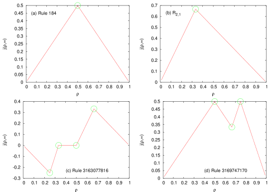
Figure 1: Examples of fundamental diagrams for number-conserving rules. Singularities are denoted by green circles. Diagrams (c) and (d) represent $n=5$ rules with indicated Wolfram’s numbers.

Quite often, fundamental diagrams of number-conserving rules consist of a finite number of linear segments separated by similar singularities, as shown in Figure 1b–d.

Since number-conserving CA rules conserve the number of occupied sites, we can label each occupied site (or “particle”) with an integer $n\in\mathbbm{Z}$, such that the closest particle to the right of particle $n$ is labeled $n+1$. If $y_{n}(t)$ denotes the position of particle $n$ at time $t$, the configuration of the particle system at time $t$ is described by the increasing bisequence $\{y_{n}(t)\}_{n=-\infty}^{\infty}$. We can then specify how the position of the particle at the time step $t+1$ depends on positions of the particle and its neighbours at the time step $t$. For example, for rule 184 one obtains

$$y_{n}(t+1)=y_{n}(t)+\min\{y_{n+1}(t)-y_{n}(t)-1,1\}.$$ (12)

Equation (12) is sometimes referred to as the motion representation. For arbitrary number-conserving CA rule it is possible to obtain the motion representation by employing algorithm described in [22]. The motion representation is analogous to Lagrange representation of the fluid flow, in which we observe individual particles and follow their trajectories. On the other hand, eq. (11) could be called Lagrange representation, because it describes the process at a fixed point in space. The Euler-Lagrange analogy has been explored in [23].

In practice, the choice between Euler and Langrange description of the number-conserving CA is usually dictated by convenience. Cellular automata rules which we want to consider in this paper are easier to define using the Euler paradigm, as we will see in the next section.

3 Anticipatory driving rules

In what follows, we will consider a class of CA rules first introduced in [17]. They are defined in terms of two positive integers $m$ (maximum speed) and $k$ (blocking parameter). These rules can be interpreted as simplified deterministic models of road traffic flow with driver’s anticipation. Occupied sites represent cars on a single-lane road. All cars move synchronously using the following algorithm. Driver of each car first locates the nearest gap (cluster of empty sites) in front of him, the length of this gap denoted by $g$. If the first empty site (i.e., the first site belonging to the aforementioned gap) is further than $k$ sites ahead, the car does not move, otherwise, it moves to the site $i+v$, where $v=\min(g,m)$. More formally, using Euler’s paradigm, and denoting position of the $n$-th car by $y_{n}(t)$, we can write

$$y_{n}(t+1)=y_{n}(t)+[[y_{b}(t)-y_{n}(t)+1\leq k]]\min\{g,m\},$$ (13)

where

$$b = \min\{i\in\mathbbm{Z}:i\geq n\mbox{\,\,and\,\,}y_{i+1}(t)-y_{i}(t)>1\},$$ (14)

$$g = y_{b+1}(t)-y_{b}(t)-1,$$ (15)

and where $[[P]]=1$ if the statement $P$ is true, otherwise $[[P]]=0$.

Cellular automaton rule defined by (13–15) will be referred to as as ${\cal R}_{m,k}$. To illustrate dynamics of this rule, let us assume that $m=k=2$. Consider, for example, the following configuration:

$\cdots$	0	0	A	B	0	0	C	0	D	0	0	$\cdots$
$\cdots$	0	0	0	0	A	B	0	C	0	0	D	$\cdots$

The first row represents configuration of cars A, B, C, D at time $t$, and the second line their configuration at time $t+1$. Zeros denote empty sites. Car B sees ahead a gap of length 2, so it will move by two sites. Car A sees the same gap, so it will move by two sites as well. As a result, cars A and B move together as if they formed a single “block”. This is called “anticipatory driving” – car A anticipates that car B will move. For rule ${\cal R}_{m,k}$, cars can move in blocks of length up to $k$.

Compare this with $m=2$, $k=1$ case:

$\cdots$	0	0	A	B	0	0	C	0	D	0	0	$\cdots$
$\cdots$	0	0	A	0	0	B	0	C	0	0	D	$\cdots$

Car A has not moved, because the first gap ahead of it begins further than $k=1$ sites away, so A cannot see it, and, as a result, cannot anticipate that B will move.

4 Known results for ${\cal R}_{m,1}$ and ${\cal R}_{1,k}$

For rules ${\cal R}_{m,1}$, $m=1,2,\ldots$, the current $j(t,\rho)$, as defined by eq. (8), can be computed explicitly. As shown in [7], it is given by

$$j(\rho,t)=1-\rho-\sum_{i=1}^{t+1}\frac{i}{t+1}{{(m+1)(t+1)}\choose{t+1-i}}\rho^{t+1-i}(1-\rho)^{m(t+1)+i}.$$ (16)

One can then show that in the limit of $t\to\infty$, the equilibrium current $j(\rho,\infty)$ is a piecewise linear function of $\rho$ given by

$$j(\rho,\infty)=\left\{\begin{array}[]{ll}m\rho&\mbox{if $\rho<1/(m+1)$},\\ 1-\rho&\mbox{otherwise},\end{array}\right.$$ (17)

as shown in Figure 1(b).

For $\rho<1/(m+1)$ the average velocity of particles at equilibrium is $m$, i.e., all particles are moving to the right with the maximum speed $m$. The system is said to be in the a free-moving phase. When $\rho>1/(m+1)$, the speed of some particles is less than the maximum speed $m$. The system is in the so-called jammed phase.

The transition from the free-moving phase to the jammed phase occurs at $\rho=\rho_{c}=1/(m+1)$ called the critical density. At $\rho_{c}$, it is possible to obtain an asymptotic approximation of (16) by replacing the sum by an integral and using de Moivre-Laplace limit theorem, as done in [7]. At $\rho_{c}$ this procedure yields

$$j(\rho,\infty)-j(\rho,t)=\sqrt{\frac{m}{2\pi(m+1)t}}\left(e^{-\frac{(m+1)}{2mt}}-e^{-\frac{(m+1)t}{2m}}\right),$$ (18)

and therefore

$$j(\rho,\infty)-j(\rho,t)\sim t^{-1/2}.$$ (19)

Here, by $f(t)\sim g(t)$ we mean that $\lim_{t\to\infty}f(t)/g(t)$ exists and is different from $0$.

Very similar results can be obtained for ${\cal R}_{1,k}$, $k=1,2,\ldots$, if one takes advantage of the duality property. Duality in this context means that if cars are moving to the right according to the rule ${\cal R}_{m,k}$, then empty sites can be treated as another type of particles which are moving to the left according to ${\cal R}_{k,m}$. Therefore, if we replace $\rho$ by $1-\rho$ in eq. (16), we will obtain the equilibrium current for ${\cal R}_{1,k}$

$$j(\rho,t)=\rho-\sum_{i=1}^{t+1}\frac{i}{t+1}{{(k+1)(t+1)}\choose{t+1-i}}(1-\rho)^{t+1-i}\rho^{k(t+1)+i},$$ (20)

and

$$j(\rho,\infty)=\left\{\begin{array}[]{ll}\rho&\mbox{if $\rho<k/(k+1)$},\\ k(1-\rho)&\mbox{otherwise}.\end{array}\right.$$ (21)

As in the case of ${\cal R}_{m,1}$, rule ${\cal R}_{1,k}$ exhibits two phases represented by linear segments of the fundamental diagram, separated by the singularity at $\rho=k/(k+1)$.

5 Rule ${\cal R}_{2,2}$

For arbitrary $m$ and $k$ both greater than $1$, explicit expressions for the equilibrium current are not known. Nevertheless, Kujala and Lukka [16] presented an efficient algorithm which can determine the steady-state current starting from a given initial state. Using that algorithm and the method of generating functions, they obtained polynomial equations relating the equilibrium current and the density.

When $m>1$ or $k>1$, the fundamental diagram for ${\cal R}_{m,k}$ is different than in the case of ${\cal R}_{m,1}$ or ${\cal R}_{1,k}$. In addition to the free moving phase and the jammed phase, a novel phase appears, which we will call an intermediate phase. The smallest values of $m$ and $k$ for which one can observe this phenomenon is $m=k=2$, and we will use these values in subsequent considerations.

For $m=k=2$, the method of [16] method yields

$$j(\rho,\infty)=\left\{\begin{array}[]{ll}2\rho&\mbox{if $\rho\leq\rho_{c1}$},\\ C&\mbox{if $\rho_{c_{1}}<\rho<\rho_{c2}$},\\ 2(1-\rho)&\mbox{if $\rho\geq\rho_{c2}$},\end{array}\right.$$ (22)

where

$$\rho_{c1} = \frac{6}{7}-\frac{2\sqrt{2}}{7},$$ (23)

$$\rho_{c2} = 1-\rho_{c1},$$ (24)

and where $C$ is a solution of

$$16C^{2}+\rho^{2}(1-\rho^{2})(8C^{2}-36C^{3})+(1+27\rho^{2}(1-\rho^{2}))C^{4}-C^{5}=0.$$ (25)

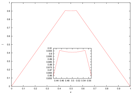
Figure 2: Fundamental diagram for rule ${\cal R}_{2,2}$ as given by eq. (22). The inset shows magnification of the non-concavity region.

Figure 2 shows the graph of $j(\rho,\infty)$ as a function of $\rho$ for rule ${\cal R}_{2,2}$. Two singularities at $\rho_{c1}$ and $\rho_{c2}$ are clearly visible. By singularities we understand values of $\rho$ for which $j(\rho,\infty)$ is non-differentiable with respect to $\rho$. The two singularities divide the fundamental diagram into three parts. When $\rho\leq\rho_{c1}$, all particles are moving with velocity $2$, so we will call this a free moving phase. The region $\rho_{c_{1}}<\rho<\rho_{c2}$ will be called an intermediate phase, and the region $\rho\geq\rho_{c2}$, in analogy to the fundamental diagram described by eq. (17), will be called a jammed phase.

The existence of singularities in fundamental diagrams of number-conserving rules is not new, and their properties have been documented in [7, 1]. The most common singularity type is a singularity which separates two linear segments of the fundamental diagram, just like $\rho=1/(m+1)$ for ${\cal R}_{m,1}$ (eq.17). At all such singularities, numerical evidence suggests that the relaxation to the equilibrium follows the same power law, i.e. $j(\rho,\infty)-j(\rho,t)\sim t^{-1/2}$.

The two singularities in rule ${\cal R}_{2,2}$ are different from the singularity observed in ${\cal R}_{m,1}$, since they separate linear segments of the fundamental diagram from the nonlinear segment. Yet surprisingly, they exhibit the same power law behaviour, as we shall see in the next section.

6 Convergence to equilibrium

In order to define current for ${\cal R}_{2,2}$, we will first write definition of ${\cal R}_{2,2}$ using Lagrange’s representation. Its local function $f$ appearing in eq. (1) can be written as in a compact form as

$$f(x_{1},x_{2},x_{3},x_{4},x_{5})=x_{1}+x_{2}x_{4}-x_{1}x_{3}-x_{1}x_{2}x_{4}-x_{2}x_{3}x_{4}+x_{2}x_{3}x_{5}$$

$$+x_{1}x_{2}x_{3}x_{4}-x_{2}x_{3}x_{4}x_{5}+x_{3}x_{4}x_{5},$$ (26)

with $l=-2$, $r=2$. The local current, as defined by eq. (4), becomes

$$J(x_{1},x_{2},x_{3},x_{4})=x_{1}+x_{2}-x_{1}x_{2}x_{4}-x_{1}x_{3}+x_{1}x_{2}x_{3}x_{4}-x_{2}x_{3}x_{4}.$$ (27)

In order to estimate the expected current $j(\rho,t)$ as defined by eq. (8), we performed a series of numerical experiments. We start with a lattice of $L=10^{6}$ sites, where initially each site is occupied with probability $\rho$ and empty with probability $1-\rho$. After $t$ iterations, the average current is then given by

$$\langle j(\rho,t)\rangle=\frac{1}{L}\sum_{i=0}^{L-1}J(s_{i}(t),s_{i+1}(t),s_{i+2}(t),s_{i+3}(t)).$$ (28)

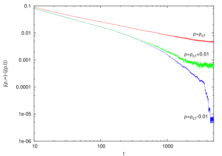
Figure 3: Graphs of $j(\rho,\infty)-\langle j(\rho,t)\rangle$ as a function of time for rule ${\cal R}_{2,2}$.

Figure 3 shows graphs of $j(\rho,\infty)-\langle j(\rho,t)\rangle$ for three different values of the density $\rho$: exactly at the singularity ($\rho=\rho_{c1}$), slightly below ($\rho=\rho_{c1}-0.01$), and slightly above ($\rho=\rho_{c1}+0.01$). Due to the symmetry of the fundamental diagram of ${\cal R}_{2,2}$, the behaviour in the vicinity of $\rho_{c_{2}}$ is the same, therefore we are only considering $\rho_{c_{1}}$. We can see that at the singularity the power law behavior is observed, as evidenced by the straight line in the log-log plot. This is not the case, however, for densities smaller or grater than than $\rho_{c1}$. For $\rho=\rho_{c1}$, fitting the curve

$$j(\rho,\infty)-\langle j(\rho,t)\rangle=At^{\alpha}$$ (29)

to the data set visualized in Figure 3, we obtain $\alpha=-0.489\pm 0.005$, which is very close to values reported previously for singularities in other number-conserving rules, and very close to the exact value $\alpha=-1/2$ known for ${\cal R}_{1,m}$. This suggests that singularities in ${\cal R}_{2,2}$ have the same nature as singularities in other number-conserving rules. To confirm this observation, we will introduce the notion of the decay time defined as

$$\tau(\rho)=\sum_{t=0}^{\infty}j(\rho,\infty)-j(\rho,t).$$ (30)

If the decay is of power-law type, i.e. $j(\rho,\infty)-\langle j(\rho,t)\rangle\sim t^{\alpha}$ with $\alpha\leq 1$, then the infinite sum in eq. (30) should diverge. If, on the other hand, the decay is exponentially fast, we should see rapid convergence. For five-input ($n=5$) number-conserving CA rules with piecewise-linear fundamental diagrams investigated in [1], the divergence of $\tau(\rho)$ has been observed only at the singularity, while away from the singularity $\tau(\rho)$ it quickly converged. Figure 4 shows graphs of the truncated decay time defined as

$$\tau_{T}(\rho)=\sum_{t=0}^{T}j(\rho,\infty)-j(\rho,t)$$ (31)

as a function of $\rho$ for several values of $T$. One can see that the decay time diverges at critical points $\rho_{c1}$ and $\rho_{c2}$, similarly as reported in [1] for other number-conserving rules.

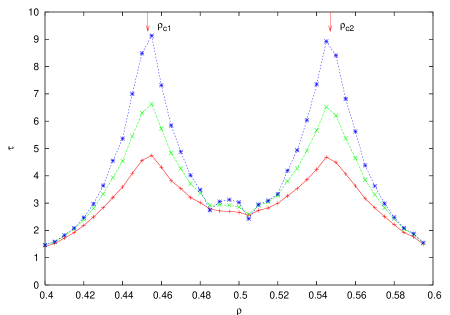
Figure 4: Truncated decay time $\tau_{T}(\rho)$ as a function of $\rho$ for $T=100$ ($+$), $T=200$ ($\times$) and $T=400$ ($\star$) for a lattice of $1000$ sites. Each point represents average of $100$ runs.

7 Phase transitions

Divergence of the decay time at the critical point $\rho_{c1}$ is somewhat similar to the critical slowing down observed in phase transitions – the closer to the singularity, the longer it takes to reach the steady state. In fact, it is possible to define the order parameter for rule ${\cal R}_{2,2}$, thus interpreting the singularity at $\rho_{c1}$ as the critical point in a second-order kinetic phase transition.

We will first note that the maximum possible current occurs when all particles are moving with the maximum speed, which for ${\cal R}_{2,2}$ is $2$, hence the maximum current is equal to $2\rho$. The natural choice of the order parameter would be therefore the difference between the maximum possible current and the actual current in the steady state. We will denote this order parameter by $M(\rho)$, formally defined as

$$M(\rho)=2\rho-j(\rho,\infty).$$ (32)

The order parameter is zero in the free-moving phase, and becomes non-zero in the intermediate phase.

Using eq. (22), it is possible to obtain series expansion of $M(\rho)$ around $\rho_{c1}$ for $\rho\geq\rho_{c1}$:

$$M(\rho)\propto(10\sqrt{2}-12)(\rho-\rho_{c1})+\frac{1}{2}(47\sqrt{2}-69)(\rho-\rho_{c1})^{2}+O((\rho-\rho_{c1})^{3}).$$ (33)

The critical exponent beta, normally defined by $M(\rho)\propto(\rho-\rho_{c1})^{\beta}$, is therefore equal to $1$. Again, this is in agreement with the value of $\beta$ obtained for other number-conserving rules [1].

8 Intermediate phase

In spite of all similarities to other number-conserving rules, the behavior of ${\cal R}_{2,2}$ is somewhat unusual, especially in the intermediate phase, where the fundamental diagram is nonlinear.

As mentioned earlier, dynamics of number-conserving CA rules somewhat resembles dynamics of the kinematic wave equation, which describes propagation of density waves in a continuous medium. For the kinematic wave equation, the slope of the fundamental diagram at a given point represents velocity of density waves. It turns out that the slope of the fundamental diagram for number-conserving CA can be interpreted in a similar way.

In the free moving phase, the slope of the fundamental diagram given by eq. (22) is equal to $\frac{\partial j}{\partial\rho}=2$. Compare this to Figure 5(a) showing the spatio-temporal diagram for $\rho=0.42$, which is in the free-moving phase. If we treat regions of alternating blocks $11$ and $00$ as the “background” $\ldots 0011001100110011\ldots$, then white structures can be clearly identified in that background. They propagate to the right with velocity $2$. These are analogs of density waves – in fact, they are regions of local density smaller than $1/2$, i.e., blocks of zeros longer than 2 or block of ones shorter than 2. Free moving phase is dominated by such density waves. On the other hand, in the jammed phase, only density waves propagating to the left with velocity $-2$ remain in the steady state, as shown in Figure 5(d). This again agrees with the slope of the fundamental diagram given by eq. (22): in the jammed phase, $\frac{\partial j}{\partial\rho}=-2$.

The intermediate phase is the most interesting one, because its dynamics is not dominated by a single type of density waves. Figures 5(b) and (c) show two examples of spatio-temporal patterns in the intermediate phase. One can clearly see that two types of density waves are present. Blocks containing isolated zeros propagate to the right, while blocks with isolated ones move to the left. When these two types collide, they both are slightly delayed, but after the collision, they continue with the pre-collision velocity. One could thus say that these density waves are somewhat similar to solitons – they preserve their shape and velocity in a collision. The balance between these two types of density waves determines the steady-state current.

(a) (b)

(c) (d)

Figure 5: Spatio-temporal patterns generated by ${\cal R}_{2,2}$ for random initial configurations with densities (a) $\rho=0.42$, (b) $\rho=0.47$, (c) $\rho=0.53$, (d) $\rho=0.58$. Vertical axis (increasing downward) represents time, while horizontal axis represents space. Blacks squares represent occupied sites.

As it turns out, this balance not only depends on the density $\rho$, but also on the amount of correlations present in the initial configuration. When the initial configuration is described by Bernoulli probability measure, i.e., all sites are independently occupied with the same fixed probability, the fundamental diagram is given by (22), and the transition to the intermediate phase occurs at $\rho_{c1}=\frac{6}{7}-\frac{2\sqrt{2}}{7}$. Yet the location of the singularity $\rho_{c1}$ strongly depends on the assumption of the initial distribution being Bernoulli.

To illustrate this, we prepared “clustered initial condition” using the following algorithm. We start with empty lattice of $L$ sites. In order to produce initial condition with $\rho L$ occupied sites, we repeat the following sequence of steps until the number of occupied sites reaches $\rho L$:

1. select one site randomly among all empty sites and make it occupied by a particle;

2. with probability $q$, move this particle to the site adjacent to the nearest occupied site, and with probability $1-q$, leave it in the initial position.

In the above, $q\in[0,1]$ is a parameter describing “clustering” of occupied sites. When $q=0$, we obtain random non-correlated configuration. When $q=1$, all occupied sites form a single continuous block.

Figure 6: Order parameter $M$ as a function of $\rho$ for $q=0$ ($+$), $q=0.2$ ($\times$), $q=0.4$ ($\star$), and $q=1$ ($\square$). Simulations performed on a lattice of $10^{4}$ sites with ${\cal R}_{2,2}$ iterated $10^{4}$ time steps. Each point represents average of $100$ runs.

Figure 6 shows the order parameter $M$ as a function of the density $\rho$ for four different values of $q$. When $q=0$, the critical point is exactly at $\rho_{c1}$, as expected. However, as $q$ increases, the critical point moves to the right, and when $q=1$, it reaches $0.5$. Obviously, the same thing happens to the second singularity, for which one could define analogous order parameter. When $q=1$, these two singularities merge and we have just one singularity at $\rho=0.5$. That means that the intermediate phase disappears as $q\rightarrow 1$.

This behavior is in sharp contrast with the behavior of number-conserving rules with piecewise-linear fundamental diagrams. For these rules, the steady-state current depends only on the density, and does not depend on the amount of spatial correlations present in the initial condition.

9 Conclusions

We investigated properties of the fundamental diagram of rule ${\cal R}_{2,2}$. This rule has been used as a representative example of a class of number-conserving rules for which the fundamental diagram is known, and for which not all segments of the fundamental diagram are linear. We found that the nature of singularities in the fundamental diagram of ${\cal R}_{2,2}$ is the same as for rules with piecewise-linear diagrams. The current converges toward its equilibrium value like $t^{-1/2}$, and the critical exponent $\beta$ is equal to $1$.

These results seem to support a more general conjecture that all singularities in number-conserving CA rules exhibit universal behavior. It is interesting to note at this point that the critical exponent $\beta=1$ is also obtained in equilibrium statistical physics in the case of second-order phase transitions with non-negative order parameter and above the upper critical dimensionality. This indicates that phase transitions in number-conserving CA are all mean-field type, and the observed universal behavior in in fact mean-field type behavior. In order to explore this issue further, it would be necessary to introduce a field conjugate to the order parameter, and then numerically compute other critical exponents such as the exponent $\gamma$ characterizing the divergence of the susceptibility at the critical point, or $\delta$, characterizing the behavior of the order parameter at the critical point when the field approaches $0$, similarly as done in [24] for the simplified Nagel-Screckenberg model. This problem is currently under investigation, and results will be reported elsewhere.

Acknowledgements: The author acknowledges financial support from NSERC (Natural Sciences and Engineering Research Council of Canada) in the form of the Discovery Grant and from SHARCNET in the form of CPU time.

References

- [1] H. Fukś and N. Boccara, “Convergence to equilibrium in a class of interacting particle systems,” Phys. Rev. E 64 (2001) 016117, arXiv:nlin.CG/0101037.
- [2] J. Krug and H. Spohn, “Universality classes for deterministic surface growth,” Phys. Rev. A 38 (1988) 4271–4283.
- [3] T. Nagatani, “Creation and annihilation of traffic jams in a stochastic assymetric exclusion model with open boundaries: a computer simulation,” J. Phys. A: Math. Gen. 28 (1999) 7079–7088.
- [4] K. Nagel, “Particle hopping models and traffic flow theory,” Phys. Rev. E 53 (1996) 4655–4672, arXiv:cond-mat/9509075.
- [5] V. Belitsky and P. A. Ferrari, “Invariant measures and convergence for cellular automaton 184 and related processes,” math.PR/9811103. Preprint.
- [6] M. S. Capcarrere, M. Sipper, and M. Tomassini, “Two-state, r=1 cellular automaton that classifies density,” Phys. Rev. Lett. 77 (1996) 4969–4971.
- [7] H. Fukś, “Exact results for deterministic cellular automata traffic models,” Phys. Rev. E 60 (1999) 197–202, arXiv:comp-gas/9902001.
- [8] K. Nishinari and D. Takahashi, “Analytical properties of ultradiscrete burgers equation and rule-184 cellular automaton,” J. Phys. A-Math. Gen. 31 (1998) 5439–5450.
- [9] V. Belitsky, J. Krug, E. J. Neves, and G. M. Schutz, “A cellular automaton model for two-lane traffic,” J. Stat. Phys. 103 (2001) 945–971.
- [10] M. Blank, “Ergodic properties of a simple deterministic traffic flow model,” J. Stat. Phys. 111 (2003) 903–930.
- [11] M. Pivato, “Conservation laws in cellular automata,” Nonlinearity 15 (2002) 1781–1793, arXiv:math.DS/0111014.
- [12] A. Moreira, “Universality and decidability of number-conserving cellular automata,” Theor. Comput. Sci. 292 (2003) 711–721.
- [13] B. Durand, E. Formenti, and Z. Róka, “Number-conserving cellular automata I: decidability,” Theoretical Computer Science 299 (2003) 523–535.
- [14] E. Formenti and A. Grange, “Number conserving cellular automata II: dynamics,” Theoretical Computer Science 304 (2003) 269–290.
- [15] K. Morita and K. Imai, “Number-conserving reversible cellular automata and their computation-universality,” Theoretical Informatics and Applications 35 (2001) 239–258.
- [16] J. V. Kujala and T. J. Lukka, “Solutions for certain number-conserving deterministic cellular automata,” Phys. Rev. E 65 (2002) art. no.–026115, arXiv:nlin.CG/0105045.
- [17] H. Fukś and N. Boccara, “Generalized deterministic traffic rules,” Int. J. Mod. Phys. C 9 (1998) 1–12, arXiv:adap-org/9705003.
- [18] D. Chowdhury, L. Santen, and A. Schadschneider, “Statistical physics of vehicular traffic and some related systems,” Physics Reports 329 (2000) 199–329.
- [19] D. Helbing, “Traffic and related self-driven many-particle systems,” Rev. Mod. Phys. 73 (2001) 1067.
- [20] T. Hattori and S. Takesue, “Additive conserved quantities in discrete-time lattice dynamical systems,” Physica D 49 (1991) 295–322.
- [21] N. Boccara and H. Fukś, “Cellular automaton rules conserving the number of active sites,” J. Phys. A: Math. Gen. 31 (1998) 6007–6018, arXiv:adap-org/9712003.
- [22] H. Fukś, “A class of cellular automata equivalent to deterministic particle systems,” in Hydrodynamic Limits and Related Topics, A. T. L. S. Feng and R. S. Varadhan, eds., Fields Institute Communications Series. AMS, Providence, RI, 2000. arXiv:nlin.CG/0207047.
- [23] J. Matsukidaira and K. Nishinari, “Euler-Lagrange correspondence of cellular automaton for traffic-flow models,” Phys. Rev. Lett. 90 (2003) art. no.–088701.
- [24] N. Boccara and H. Fukś, “Critical behavior of a cellular automaton highway traffic model,” J. Phys. A: Math. Gen. 33 (2000) 3407–3415, arXiv:cond-mat/9911039.