Conservation and dynamics of blocks 10 in the cellular automaton rule 142

1 Introduction

Let $s$ be a binary string of $L$ symbols, i.e., $s=s_{0}s_{1}\ldots s_{L-1}$, where $s_{i}\in\{0,1\}$ for $0\leq i\leq L$, $L\in{\mathbbm{N}}$. We will say that the symbol $s_{i}$ has a dissenting right neighbour if $s_{i-1}=s_{i}\neq s_{i+1}$. By flipping a given symbol $s_{i}$ we will mean replacing it by $1-s_{i}$.

Consider now the following problem: suppose that we simultaneously flip all symbols which have dissenting right neighbours, as shown in the example below.

$$\begin{array}[]{cccccccccccccc}\cdots&0&0&1&0&0&1&1&1&0&1&0&1&\cdots\\ &&\Big{\downarrow}&&&\Big{\downarrow}&&&\Big{\downarrow}&&&&&\\ \cdots&0&1&1&0&1&1&1&0&0&1&0&1&\cdots\end{array}$$ (1)

Assuming that the initial string is randomly generated, what is the probability that a given symbol has a dissenting right neighbour after $t$ iterations of the aforementioned procedure?

In order to answer this question, we will take advantage of the fact that the process described in the previous paragraph is actually a cellular automaton rule 142, using Wolfram’s numbering scheme for elementary cellular automata [1]. It has a property which turns out to be crucial to the solution. If one counts the number of pairs $10$ in (1) before and after the bit-flipping operation, it is easy to see that this number remains constant (similarly as the number of pairs $01$). We will show that this is true for an arbitrary string, and we will take advantage of this fact to compute the probability of having a dissenting neighbour.

2 Definitions

Before we proceed, we will introduce several concepts of cellular automata theory. Let ${\cal G}=\{0,1\}$ be called a symbol set, and ${\cal S}=\{0,1\}^{{\mathbbm{Z}}}$ be called the configuration space. A block of radius $r$ is an ordered set $b_{-r}b_{-r+1}\ldots b_{r}$, where $r\in{\mathbbm{N}}$, $b_{i}\in{\cal G}$. Let $r\in{\mathbbm{N}}$ and let ${\cal B}_{r}$ denote the set of all blocks of radius $r$ over ${\cal G}$. The number of elements of ${\cal B}_{r}$ (denoted by $\mathop{\rm{card}}{\cal B}_{r}$) equals $2^{2r+1}$.

A mapping $f:\{0,1\}^{2r+1}\mapsto\{0,1\}$ will be called a cellular automaton rule of radius $r$. Alternatively, the function $f$ can be considered a mapping of ${\cal B}_{r}$ into ${\cal B}_{0}={\cal G}=\{0,1\}$.

Corresponding to $f$ (also called a local mapping), we define a global mapping $F:S\to S$ such that $(F(s))_{i}=f(s_{i-r},\ldots,s_{i},\ldots,s_{i+r})$ for any $s\in S$. The composition of two rules $f,g\in{\cal F}$ can be now defined in terms of their corresponding global mappings $F$ and $G$ as $(F\circ G)(s)=F(G(s)),$ where $s\in S$. We note that if $f\in{\cal F}_{p}$ and $g\in{\cal F}_{q}$, then $f\circ g\in{\cal F}_{p+q}$. For example, the composition of two radius-1 mappings is a radius-2 mapping:

$$(f\circ g)(s_{-2},s_{-1},s_{0},s_{1},s_{2})=f(g(s_{-2},s_{-1},s_{0}),g(s_{-1},s_{0},s_{1}),g(s_{0},s_{1},s_{2})).$$ (2)

Multiple composition will be denoted by

$$f^{n}=\underbrace{f\circ f\circ\cdots\circ f}_{\mbox{$n$ times}}.$$ (3)

A block evolution operator corresponding to $f$ is a mapping ${\rm\bf f}:{\cal B}\mapsto{\cal B}$ defined as follows. Let $r\geq p>0$, $a\in{\cal B}_{r}$, $f\in{\cal F}_{p}$, and let $b_{i}=f(a_{i-p},a_{i-p+1},\ldots,a_{i+p})$ for $-r+p\leq i\leq r-p$. Then we define ${\rm\bf f}(a)=b$, where $b\in{\cal B}_{r-p}$. Note that if $b\in B_{1}$ then $f(b)={\rm\bf f}(b)$.

In this paper, we will be concerned with trajectories of a given configuration under consecutive iterations of $F$. Denoting the initial configuration by $s(0)$, the image of $s(0)$ after $t$ iterations of $F$ will be denoted by $s(t)$, i.e.,

$$s(t)=F^{t}(s(0)),$$ (4)

which imples that

$$s(t+1)=F(s(t)),$$ (5)

and hence

$$s_{i}(t+1)=f(s_{i-r}(t),s_{i-r+1}(t),\ldots,s_{i+r}(t)).$$ (6)

Cellular automaton rule 142, which is the subject of this paper, has the following local function

$$f(0,0,0)=0,f(0,0,1)=1,f(0,1,0)=1,f(0,1,1)=1,$$ (7)

$$f(1,0,0)=0,f(1,0,1)=0,f(1,1,0)=0,f(1,1,1)=1,$$

which can also be written in an algebraic form

$$f(x_{0},x_{1},x_{2})=x_{1}+(1-x_{0})(1-x_{1})x_{2}-x_{0}x_{1}(1-x_{2}).$$ (8)

3 Conservation

As shown in [2], rule 142 is one of the few nontrivial elementary rules which posses the second order additive invariant. It conserves the number of blocks $10$, and this fact can be formally described as follows. Let us first define a function $\xi(x_{0},x_{1})=x_{0}(1-x_{1})$, which takes value $1$ on block $10$ and value $0$ on all other blocks of length $2$. We will call $\xi$ the density of blocks $10$. Following [3], we will say that $\xi$ is a density function of an additive invariant of $f$ if

$$\sum_{i=0}^{L-1}\xi(f(s_{i},s_{i+1},s_{i+2}),f(s_{i+1},s_{i+2},s_{i+3}))=\sum_{i=0}^{L-1}\xi(s_{i},s_{i+1})$$ (9)

for every positive integer $L$ and for all $s_{0},s_{1},\ldots,s_{L-1}\in\{0,1\}$. In the above, and in all subsequent considerations, we are assuming that addition of all spatial indices is performed modulo $L$. That is, we will be concerned with periodic configurations, or, in other words, configurations with periodic boundary conditions where $s(i+L)=s(i)$ for all integers $i$.

The right hand side of the above equation simply denotes the number of blocks $10$ in the configuration $s=(s_{0},s_{1},\ldots,s_{L-1})$, and the left hand side denotes the number of these blocks in the image of $s$ under $f$.

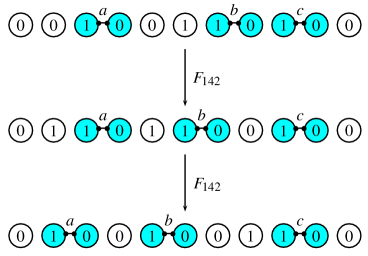
Figure 1: Two consecutive images of a sample configuration under rule 142, assuming periodic boundary conditions. Blocks $10$ are labelled with letters a,b,and c.

Figure 1 shows an example of a configuration $s$ consisting of 11 sites, and its two consecutive images under rule 142, i.e., $F_{142}(s)$ and $F^{2}_{142}(s)$, where $F_{142}$ denotes the global function of rule 142. Periodic boundary conditions are assumed. The initial configuration $s$ contains three blocks $10$ labelled $a$, $b$, and $c$, and one can clearly see that the number of blocks $10$ remains constant after each application of $F_{142}$. Moreover, since the number of blocks $10$ remains constant, we can label them with distinctive labels, which will allow us to keep track of individual blocks. In Figure 1, such labelling can be simply obtained by enumerating blocks $10$ from left to right. For example, looking again at Figure 1, we could say that block $a$ remains in the same position after the first iteration, but moves to the left by one site in the second iteration. Similarly, block $b$ moves by one site to the left in both iterations shown in Figure 1.

To formalize the concept of the motion of blocks, we will first prove that rule 142 conserves the number of blocks $10$ in an arbitrary periodic configuration. Let us note that

$$\xi(f(s_{i},s_{i+1},s_{i+2}),f(s_{i+1},s_{i+2},s_{i+3}))=$$ (10)

$$f(s_{i},s_{i+1},s_{i+2})(1-f(s_{i+1},s_{i+2},s_{i+3})).$$

Using (8), the right hand side of the above equation becomes somewhat complicated, but it drastically simplifies if one notes that all variables $s_{i}$ in this equation are Boolean, and $x^{n}=x$ for all positive $n$ if $x\in\{0,1\}$. After this simplification, one obtains

$$\xi(f(s_{i},s_{i+1},s_{i+2}),f(s_{i+1}, s_{i+2},s_{i+3}))=$$

$$-s_{i}s_{i+1}+s_{i+1}+ s_{i}s_{i+1}s_{i+2}-s_{i+1}s_{i+2}s_{i+3}.$$ (11)

We will now regroup terms on the right hand side

$$\xi(f(s_{i},s_{i+1},s_{i+2}),f(s_{i+1},s_{i+2},s_{i+3})) =$$

$$s_{i+1}(1-s_{i+2})+s_{i+1}s_{i+2}(1-s_{i+3}) -s_{i}s_{i+1}(1-s_{i+2}),$$ (12)

and finally write the last equation as

$$\xi(f(s_{i},s_{i+1}, s_{i+2}),f(s_{i+1},s_{i+2},s_{i+3}))=$$ (13)

$$\xi(s_{i+1},s_{i+2}))-J(s_{i+1},s_{i+2},s_{i+3})+J(s_{i},s_{i+1},s_{i+2}),$$

where

$$J(x_{0},x_{1},x_{2})=x_{0}x_{1}(x_{2}-1).$$ (14)

This leads to

$$\sum_{i=0}^{L-1}\xi(f(s_{i},s_{i+1},s_{i+2}),f(s_{i+1},s_{i+2},s_{i+3}))=\sum_{i=0}^{L-1}\xi(s_{i+1},s_{i+2})\\ -\sum_{i=0}^{L-1}J(s_{i+1},s_{i+2},s_{i+3})+\sum_{i=0}^{L-1}J(s_{i},s_{i+1},s_{i+2}),$$ (15)

and, since $\sum_{i=0}^{L-1}J(s_{i+1},s_{i+2},s_{i+3})=\sum_{i=0}^{L-1}J(s_{i},s_{i+1},s_{i+2})$, the conservation condition (9) follows.

The equation(13) resembles continuity equation, with $J$ playing a role of current, or flow of blocks $10$ [3]. To see this, let us note that $J(s_{i}(t),s_{i+1}(t),s_{i+2}(t))$ takes non-zero value only when $s_{i}(t)$,$s_{i+1}(t)$, $s_{i+2}(t)=1,1,0$. Consider now a configuration containing block $110$, surrounded by sites of undetermined state. Using definition of the local function for rule 142 (7), we can construct partial state of the configuration at the next time step. Denoting by $*$ an arbitrary value in the set $\{0,1\}$, we have $f(*,1,1)=1$, $f(1,1,0)=0$, and $f(1,0,*)=0$, hence

$$s(t)= \ldots\mathtt{110}\ldots$$ (16)

$$s(t+1)= \ldots\mathtt{100}\ldots$$

We can clearly see that the block $10$, when preceded by 1, moves by one site to the left in a single iteration. Similar argument could be used to demonstrate that the block $10$ preceded by 0 does not move:

$$s(t)= \ldots\mathtt{010}\ldots$$ (17)

$$s(t+1)= \ldots\mathtt{?10}\ldots,$$

where “$?$” denotes undetermined value. Additionally, note there is no other way to obtain the block $10$ in $s(t+1)$, that is, if $s_{i}(t+1)s_{i+1}(t+1)=10$, then we must have either $s_{i}(t)s_{i+1}(t)s_{i+2}(t)=110$ or $s_{i-1}(t)s_{i}(t)s_{i+1}(t)$ $=010$. This demonstrates that indeed only blocks $110$ can contribute to the current, in agreement with eq. (14).

4 Initial distribution

Let us now go back to the problem stated in the introduction. In order to make the problem well posed, we need to define the probability distribution $\mu$ from which the initial string is drawn. Since we know that the rule 142 conserves the number of blocks $10$, it is natural to consider an initial distribution parameterized by the density of blocks $10$. Let us define the expected value of $\xi$ at site $i$ as

$$\rho(i,t)=E_{\mu}\left[\xi(s_{i}(t),s_{i+1}(t))\right]=E_{\mu}\left[s_{i}(t)(1-s_{i+1}(t))\right].$$ (18)

Assuming that the initial distribution $\mu$ is translation-invariant, $\rho(i,t)$ will not depend on $i$, and we will therefore define $\rho(t)=\rho(i,t)$. Furthermore, since $\xi$ is density function of a conserved quantity, $\rho(t)$ is $t$-independent, so we define $\rho=\rho(t)$.

The desired distribution parameterized by $\rho$ can be obtained as follows. Let $\rho\in[0,1/2]$ be the target density of blocks $10$, and let $\{X_{i}\}_{i=0}^{L-1}$ be a collection of identical independently distributed Bernoulli random variables such that

$$Pr(X_{i}=1) =2\rho,$$ (19)

$$Pr(X_{i}=0) =1-2\rho,$$ (20)

for all $i\in\{0,1\}$. The initial configuration will be given by

$$s_{i}(0)=\left(\sum_{j=0}^{i}X_{j}\right)\mod 2.$$ (21)

Note that when $X_{i}==1$, we obtain either a subsequence $s_{i}(0)s_{i+1}(0)=01$ or $s_{i}(0)s_{i+1}(0)=10$. Those subsequences occur at the same frequency, which accounts for the factor of 2 in eq. (19).

Let $P_{t}(b)$ denote the probability of occurrence of block the $b$ in the configuration $s(t)$. If the density of blocks $10$ in the initial configuration is $\rho$, then the probability of having a dissenting neighbour at time $t$ will be denoted by $P_{\mathrm{dis}}(\rho,t)$. A site $s_{i}$ has a dissenting right neighbour if $s_{i-1}s_{i}s_{i+1}=110$ or $s_{i-1}s_{i}s_{i+1}=001$. $P_{\mathrm{dis}}(\rho,t)$ is therefore given by

$$P_{\mathrm{dis}}(\rho,t)=P_{t}(110)+P_{t}(001).$$ (22)

Although two block probabilities appear on the right hand side of the above definition, we will show that $P_{\mathrm{dis}}(\rho,t)$ can be expressed in terms of a single block probability.

As a first step, we note that the following properties are direct consequences of the definition (21).

Proposition 1

Let $P_{o}(b)$ denotes the probability of occurrence of block $b$ in the configuration drawn from the distribution given by (21). Then we have:

• $P_{0}(1)=P_{0}(1)=1/2$

• $P_{0}(10)=P(01)=\rho$

• $P_{0}(b)=P_{0}(\bar{b})$, where $\bar{b}$ denotes Boolean conjugation of block $b$, i.e. $\bar{b}_{i}=1-b_{i}$.

Rule142 exhibits Boolean self-conjugacy, that is, replacing all zeros by ones and vice versa in the definition (7) does not change the definition. This fact together with Proposition 1(iii) implies that $P_{t}(110)=P_{t}(001)$, hence

$$P_{\mathrm{dis}}(\rho,t)=2P_{t}(110).$$ (23)

Kolmogorov consistency conditions for block probabilities require that

$$P_{t}(110)+P_{t}(111) = P_{t}(11),$$

$$P_{t}(10)+P_{t}(11) = P_{t}(1),$$

hence

$$P_{t}(110)=P_{t}(1)-P_{t}(10)-P_{t}(111).$$ (24)

Using the fact that $P_{t}(10)=\rho$, we obtain

$$P_{\mathrm{dis}}(\rho,t)=2P_{t}(1)-2\rho-2P_{t}(111).$$ (25)

The next result will lead to the elimination of $P_{t}(1)$ from the above equation.

Proposition 2

Let the initial configuration $s(0)$ be drawn from the distribution given by (21), and let $s(t)$ be obtained from $s(0)$ by iterating rule 142 $t$ times, so that $s(t)=F_{142}^{t}(s(0))$. Then we have

$$P_{t}(1)=P_{t}(0)=1/2.$$ (26)

We will prove this by induction. Obviously, $P_{0}(1)=P_{0}(0)=1/2$ by Proposition 1. Let us assume that $P_{t}(1)=1/2$ for some $t$. Block $1$ has four preimages under $\mathbf{f}_{142}$, and these are $001$, $010$, $011$, $111$. This leads to

$$P_{t+1}(1)=P_{t}(001)+P_{t}(010)+P_{t}(011)+P_{t}(111).$$ (27)

Kolmogorov consistency conditions require that $P_{t}(011)+P_{t}(111)=P_{t}(11)$, and, as remarked before, Boolean self-conjugacy of the rule 142 implies $P_{t}(001)=P_{t}(110)$. This yields

$$P_{t+1}(1)=P_{t}(110)+P_{t}(010)+P_{t}(11).$$ (28)

Using consistency conditions again we get

$$P_{t+1}(1)=P_{t}(10)+P_{t}(11)=P_{t}(1),$$ (29)

and this, by induction hypothesis, yields $P_{t+1}(1)=1/2$, concluding the proof.

Proposition 2 simplifies eq. (25) to

$$P_{\mathrm{dis}}(\rho,t)=1-2\rho-2P_{t}(111).$$ (30)

Now the only thing left is to compute the probability of occurrence of block 111 in the configuration $s(t)$.

5 Preimages

In order to compute $P_{t}(111)$, we will use some properties of preimages of the block $111$. Let $\mathbf{f}^{-1}_{142}(111)$ be a set of preimages of $111$ under $\mathbf{f}_{142}$. Then we have

$$P_{t}(111)=\sum_{b\in\mathbf{f}^{-1}_{142}(111)}P_{t-1}(b).$$ (31)

Generalizing the above, we can write

$$P_{t}(111)=\sum_{b\in\mathbf{f}^{-t}_{142}(111)}P_{0}(b),$$ (32)

where again $\mathbf{f}^{-t}_{142}(111)$ is a set of preimages of $111$ under $\mathbf{f}_{142}^{t}$, i.e., under $t$ iterations of $\mathbf{f}_{142}$. To find $P_{t}(111)$ using the above property, two steps are needed: first, we have to find the set of preimages of $111$, and then to find probabilities of their occurrences in the initial distribution.

Figure 2: Tree of preimages of the block $111$ under rule 142.

Figure 2 shows three levels of preimages of $111$. Upon inspection of this figure, two properies become apparent.

Proposition 3

Let $b$ be a $t$-step preimage of 111”, that is, $b\in\mathbf{f}_{142}^{-t}(111)$. Then

• The length of $b$ is $3+2t$;

• $b$ ends with $111$.

The first property is an obvious consequence of the definition of $\mathbf{f}_{142}^{t}$, and the second one can be easily proved by induction (omitted here).

Further inspection of Figure 2 leads to the necessary and sufficient condition for a block $b$ to be a $t$-step preimage of $111$. Before stating this condition formally, we will explain it using an example.

Consider the block $b=011100111$, which is a preimage of $111$ in three steps since $\mathbf{f}_{142}(011100111)=1100111$, $\mathbf{f}_{142}(1100111)=00111$, and $\mathbf{f}_{142}(00111)=111$. Let us now assume that we start with a “capital” of $1$. We will move along the string $b=b_{0}b_{1}\ldots b_{8}$ starting from $i=6$ and moving in the direction of decreasing $i$. Every time we see that $b_{i-1}$ is different from $b_{i}$, we decrease out “capital” by $1$. If $b_{i-1}=b_{i}$, we increase our “capital” by $1$. We stop at $i=1$.

Clearly, it is possible to traverse $b=011100111$ following this procedure without making the capital negative. It turns out that this is a general property of preimages of $111$. If $b$ is a preimage of $111$, then it is possible to traverse it keeping the capital non-negative. If $b$ is not a preimage of $111$, the capital will become negative at some point. A more formal statement of this property is as follows.

Proposition 4

Let $t$ be a non-negative integer, and let $b=b_{0}b_{1}\ldots b_{2t+2}$ be a binary string of length $3+2t$ ending with $111$. Define $\chi$ to be a function of two variables such that $\chi(u,v)=1$ if $u=v$, and $\chi(u,v)=-1$ otherwise. The string $b$ is a preimage of $111$ under $\mathbf{f}_{142}^{t}$ if and only if the inequality

$$1+\sum_{i=0}^{k}\chi(b_{2t-i-1},b_{2t-i})\geq 0$$ (33)

is satisfied for all $k=0,1,\ldots,2t-1$.

Instead of proving this proposition directly, we will show that it can be derived from a similar result previously obtained for a related cellular automaton rule.

6 Rule 226

In [5] it has been observed that

$$f_{60}\circ f_{142}=f_{226}\circ f_{60},$$ (34)

where

$$f_{60}(x_{0},x_{1},x_{2}) =x_{0}+x_{1}\mod 2$$ (35)

$$f_{226}(x_{0},x_{1},x_{2}) =x_{0}x_{1}-x_{1}x_{2}+x_{2}.$$ (36)

This means that there exists a local mapping (rule 60) which transforms rule 142 into rule 226. The above correspondence between rules 142 and 226 has been illustrated in Figure 3, which shows spatiotemporal patters of rule 142 (left panel) as well as images of these patterns under the rule 60 (right panel). The patterns in the right panel are in fact identical to spatiotemporal patterns which one would obtain by iterating rule 226, providing that the initial configuration in the right panel has been obtained by applying rule 60 to the corresponding initial configuration from the left panel.

Figure 3: Spatiotemporal patterns generated by the rule 142 and their transformations under the rule 60. Densities of blocks $10$ are (a) $\rho=0.23$, (b) $\rho=0.25$, and (c) $\rho=0.26$. All patterns show 100 consecutive iterations of a lattice of 100 sites with periodic boundary conditions. Black squares represent $1$, white spaces represent $0$.

Rule 226 and its image under spatial reflection, rule 184, are the only non-trivial elementary number-conserving rules, and many results regarding their dynamics have been established [6, 7, 8, 9, 10, 11, 12, 1, 13]. For our purpose, one such result will be particularly useful.

Proposition 5

Under the rule 226, $t$ step preimages of 00 have the following properties:

• In each preimage, the number of zeros exceeds the number of ones.

• The block $a_{0}a_{1}\ldots a_{2t+1}$ is an $t$-step preimage of $00$ if and only if it ends with two zeros and

  $$1+\sum_{i=2}^{k}\xi(s_{2t+1-i})\geq 0$$ (37)

  for every $2\leq k\leq 2t+1$, where $\xi(0)=1$, $\xi(1)=-1$.

• The number of $t$-step preimages of 00 containing exactly $n_{0}$ zeros and $n_{1}$ ones is equal to

  $$\frac{n_{0}-n_{1}}{n_{0}+n_{1}}\binom{n_{0}+n_{1}}{n_{1}},$$ (38)

  where $n_{0}+n_{1}=2t+2$.

Proof of this result can be found in [14], with further generalization in [11]. The proof is based on the fact that the enumeration of preimages of $00$ under rule 226 (or 184) is equivalent to the problem of enumeration of planar lattice paths between two points, subject to some constraining conditions. This path enumeration problem can then be solved using combinatorial methods.

We will now relate preimages of rules 226 and 142.

Proposition 6

The number of $t$ step preimages of 111 under rule 142 is equal to the number of $t$ step preimages of 00 under rule 226.

We will explicitly construct a bijection $T$ between $\mathbf{f}^{-t}_{142}(111)$ and $\mathbf{f}^{-t}_{226}(00)$. Let $x$ be a block of length $m$, $b_{0}b_{1},\ldots,b_{m-1}$. We define

$$[T(x)]_{i}=x_{i}+x_{i+1}\mod 2$$ (39)

for $i=0,1,\ldots,m-2$. $T(x)$ is therefore a block of length $m-1$. Since $T$ is a block evolution operator of rule 60, relationship similar to (34) must hold, i.e.

$$T\circ\mathbf{f}_{142}=\mathbf{f}_{226}\circ T.$$ (40)

Let us now assume that $b$ is a $t$-step preimage of 111 under $\mathbf{f}_{142}$. This means that $\mathbf{f}^{t}_{142}(b)=111$. Since $T(111)=00$, we have $T(\mathbf{f}^{t}_{142}(b))=00$. Using (40) we obtain $\mathbf{f}^{t}_{226}(T(b))=00$. This means that if $b$ is a $t$-step preimage of 111 under $\mathbf{f}_{142}$, then $T(b)$ is a $t$ step preimage of 00 under100 rule 226.

Now let us consider a transformation inverse to $T$. In general, $T$ is not invertible, but if restricted to the set of preimages of 111 under $\mathbf{f}_{142}$, it becomes invertible.

For an arbitrary block $y$, there exist two different blocks $x$ such that $T(x)=y$, and one can show that these two blocks are related by Boolean conjugacy. For example, we have $T(111)=00$ and $T(000)=00$. We have to define $T^{-1}$ such that this ambiguity is removed. This can be done as follows. Let $a$ be a $t$-step preimage of 00 under rule 226, $a=a_{0}a_{1}\ldots a_{2t+1}$. We define

$$[T^{-1}(a)]_{2t+2} =1$$

$$[T^{-1}(a)]_{2t+1} =1+a_{2t+1}\mod 2$$

$$[T^{-1}(a)]_{2t} =1+a_{2t}+a_{2t+1}\mod 2$$

$$\cdots$$

$$[T^{-1}(a)]_{0} =1+a_{0}+a_{1}+\ldots+a_{2t+1}\mod 2,$$

or in a general form

$$[T^{-1}(a)]_{i}=\begin{cases}1+\displaystyle\sum_{j=i}^{2t+1}a_{j}\mod 2&\text{ if $i=0,1,\ldots,2t+1$},\\ 1&\text{if $i=2t+2$}\end{cases}.$$ (41)

One can easily show that the above transformation is indeed an inverse of $T$, and in addition we guarantee that when $a$ ends with two zeros, $T^{-1}(a)$ ends with three ones, are required for an $t$-step preimage of 111 under rule 142.

Now, if $a$ is a $t$-step preimage of 00 under rule 226, we have $\mathbf{f}^{t}_{226}(a)=00$, hence $\mathbf{f}^{t}_{226}(T(T^{-1}(a)))=00$, and by eq. (40) we obtain $T(\mathbf{f}^{t}_{142}(T^{-1}(a)))=00$. The last equation implies that $\mathbf{f}^{t}_{142}(T^{-1}(a))=111$, which means that $T^{-1}(a)$ is an $t$-step preimage of 111 under rule 142, as required. $\square$

Proposition 4 follows form the above result and Proposition 5(ii).

7 Probability of occurrence of 111

The bijective transformation $T$ constructed in in the proof of Proposition 6 has a property which will be useful in computing $P_{t}(111)$. Let us call the block $x=x_{0}x_{1}$ a matching pair if $x_{0}=x_{1}$, and a mismatched pair if $x_{0}\neq x_{1}$. If $a=T(b)$, then the number of matching pairs in $b$ is equal to the number of zeros in $a$, while the number of mismatched pairs in $b$ is equal to the number of ones in $a$. This fact, together with Proposition 5 immediately leads to the conclusion that under the rule 142, the number of $t$-step preimages of 111 with exactly $n_{0}$ matching pairs and $n_{1}$ mismatched pairs is equal to

$$\frac{n_{0}-n_{1}}{n_{0}+n_{1}}\binom{n_{0}+n_{1}}{n_{1}},$$ (42)

where $n_{0}+n_{1}=2t+2$. Probability of occurrence of a matching pair in a in the initial configuration drawn from the initial distribution is $2\rho$, and the mismatched pair is $1-2\rho$. Therefore, the probability of occurrence of a block with prescribed sequence of matching and mismatched pairs such that it has exactly $n_{0}$ matching pairs and $n_{1}$ mismatched pairs is equal to $(2\rho)^{n_{1}}(1-2\rho)^{n_{0}}$. This implies that the probability that a block of length $2t+3$, randomly selected from the distribution (21), is a $t$-step preimage of 111 with exactly $n_{0}$ matching pairs is equal to

$$\left(\frac{1}{2}\right)\frac{n_{0}-n_{1}}{n_{0}+n_{1}}\binom{n_{0}+n_{1}}{n_{1}}(2\rho)^{n_{1}}(1-2\rho)^{n_{0}}=$$

$$\frac{n_{0}-n_{1}}{4t+4}\binom{2t+2}{n_{1}}(2\rho)^{n_{1}}(1-2\rho)^{n_{0}}.$$ (43)

The factor $1/2$ in front comes from the fact that there are always two strings with a given sequence of pairs (related by Boolean conjugacy), but only one of them is a preimage of 111.

The smallest possible number of matching pairs in a $t$-step preimage of 111 is $t+2$ (recall that the number of matching pairs must exceed the number of mismatched pairs), while the maximum possible number is $2t+2$ (all zeros). Summing (7) over $n_{0}$ we obtain

$$P_{t}(111)=\sum_{n_{0}=t+2}^{2t+2}\frac{n_{0}-(2t+2-n_{0})}{4t+4}\binom{2t+2}{2t+2-n_{0}}(2\rho)^{2t+2-n_{0}}(1-2\rho)^{n_{0}}.$$ (44)

Introducing a new summation index $j=n_{0}-(t+1)$ we get

$$P_{t}(111)=\sum_{j=1}^{t+1}\frac{j}{2t+2}\binom{2t+2}{t+1-j}(2\rho)^{t+1-j}(1-2\rho)^{t+1+j},$$ (45)

and as a result, the probability (30) becomes

$$P_{\mathrm{dis}}(\rho,t)=1-2\rho-\sum_{j=1}^{t+1}\frac{j}{t+1}\binom{2t+2}{t+1-j}(2\rho)^{t+1-j}(1-2\rho)^{t+1+j},$$ (46)

where $\rho\in[0,1/2]$.

8 Equilibrium probability

We will now show how to obtain the equilibrium probability, i.e., $\lim_{t\to\infty}P_{\mathrm{dis}}(\rho,t)$. In order to find the limit $\lim_{t\rightarrow\infty}P_{t}(111)$ we can write eq. (45) in the form

$$P_{t}(111)=\sum_{j=1}^{t+1}\frac{j}{2t+2}b(t+1-j,2(t+1),2\rho),$$ (47)

where

$$b(k,n,p)=\binom{n}{k}p^{k}(1-p)^{n-k}$$ (48)

is the distribution function of the binomial distribution. Using de Moivre-Laplace limit theorem, binomial distribution for large $n$ can be approximated by the normal distribution

$$b(k,n,p)\sim\frac{1}{\sqrt{2\pi np(1-p)}}\exp{\frac{-(k-np)^{2}}{2np(1-p)}}.$$ (49)

To simplify notation, let us define $T=t+1$. Now, using (49) to approximate $b(T-j,2T,2\rho)$ in (47), and approximating sum by an integral, we obtain

$$P_{t}(111)=\int_{1}^{T}\frac{x}{2T}\frac{1}{\sqrt{8\pi T\rho(1-2\rho)}}\exp{\frac{-(T-x-4T\rho)^{2}}{8T\rho(1-2\rho)}}dx.$$ (50)

Integration yields

$$P_{t}(111) =$$

$$\sqrt{\frac{\rho(1-2\rho)}{2\pi T}}\left\{\exp\left(\frac{-(1-T+4\rho T)^{2}}{8T\rho(1-2\rho)}\right)-\exp\left({\frac{-2\rho T}{2(1-2\rho)}}\right)\right\}+$$

$$\frac{1}{4}(1-4\rho)\left\{{\rm erf}\left(\frac{4\rho T}{\sqrt{8\rho(1-2\rho)T}}\right)-{\rm erf}\left(\frac{1-T+4\rho T}{\sqrt{8\rho(1-2\rho)T}}\right)\right\},$$

where ${\rm erf}(x)$ denotes the error function

$${\rm erf(x)}=\frac{2}{\sqrt{\pi}}\int_{0}^{x}e^{-t^{2}}dt.$$ (51)

The first term in the above equation (involving two exponentials) tends to $0$ with $T\rightarrow\infty$. Moreover, since $\lim_{x\rightarrow\infty}{\rm erf}(x)=1$, we obtain

$$\lim_{t\rightarrow\infty}P_{t}(111)=\frac{1}{4}(1-4\rho)\left\{1-\lim_{T\rightarrow\infty}{\rm erf}\left(\frac{1-T+4\rho T}{\sqrt{8\rho(1-2\rho)T}}\right)\right\}.$$

Now, noting that

$$\lim_{T\rightarrow\infty}{\rm erf}\left(\frac{1-T+4\rho T}{\sqrt{8\rho(1-2\rho)T}}\right)=\left\{\begin{array}[]{ll}1,&\mbox{if $4\rho\geq 1$},\\ -1,&\mbox{otherwise},\end{array}\right.$$ (52)

we obtain

$$\lim_{t\rightarrow\infty}P_{t}(111)=\left\{\begin{array}[]{ll}1/2-2\rho&\mbox{if $\rho<1/4$},\\ 0&\mbox{otherwise}.\end{array}\right.$$ (53)

The final expression for the equilibrium probability becomes

$$\lim_{t\rightarrow\infty}P_{\mathrm{dis}}(\rho,t)=\left\{\begin{array}[]{ll}2\rho&\mbox{if $\rho<1/4$},\\ 1-2\rho&\mbox{otherwise}.\end{array}\right.$$ (54)

9 Current

The equilibrium probability calculated in the the previous section exhibits a singularity at $\rho=1/4$. This singularity is of a similar nature as the jamming transition observed in CA rules 184, 226, and related models.

Recall that in section 3 we defined the current $J$ (eq. 14). The expected value of the current is $i$-independent, so we can define the expected current as

$$j(\rho,t)=E_{\mu}\big{[}J(s_{i}(t),s_{i+1}(t),s_{i+2}(t))\big{]}=E_{\mu}\left[s_{i}(t)s_{i+1}(t)(s_{i+2}(t)-1)\right].$$ (55)

The graph of $j(\rho,\infty)$ as a function of $\rho$ is known as fundamental diagram. Using the notion of block probabilities we can rewrite (55) in an alternative form as

$$j(\rho,t)=-P_{t}(110),$$ (56)

and using (23)

$$j(\rho,t)=-\frac{1}{2}P_{\mathrm{dis}}(\rho,t).$$ (57)

The probability of having a dissenting neighbour, as we can see, is proportional to the expected current.

Since the current $J$ represents the flow of blocks $10$, the expected current must be equal to

$$j(\rho,t)=\rho v(\rho,t),$$ (58)

where $v(\rho,t)$ is the expected velocity of a block $10$ at time $t$. Using (54) this velocity is given by

$$\lim_{t\rightarrow\infty}v(\rho,t)=\left\{\begin{array}[]{ll}-1&\mbox{if $\rho<1/4$},\\ 1-\frac{1}{2\rho}&\mbox{otherwise}.\end{array}\right.$$ (59)

We can see that for densities of blocks $10$ smaller than $1/4$, the average velocity remains constant and equal to $-1$, which means that all blocks are moving to the left. At $\rho=1/4$ a jamming transition occurs, and when $\rho$ increases beyond $1/4$, more and more blocks are stopped. This phenomenon is very similar to jamming transitions in discrete models of traffic flow, which have been extensively studied in recent years ([15] and references therein).

10 Conclusions

We investigated dynamics of the cellular automaton rule 142. It can be transformed into rule 226 by a surjective transformation, which turns out to be invertible if restricted to preimages of $111$. This transformation allows to compute the probability of having a dissenting neighbour, which, in turn, allows to compute the expected current of blocks $10$. Rule 142 exhibits jamming transition similar to transitions occurring in discrete models of traffic flow.

It is worth mentioning that there are other CA rules conserving the number of blocks $10$ which also exhibit singularities of fundamental diagrams, for example rules 35 and 14, as reported in [2]. For these rules, however, there exist no transformation relating them to other rules with singularities, thus the method presented in this paper cannot be easily applied. Nevertheless, the nature of singularities in these rules appears to be the same, thus some relationship between them and rules 184/226 may exist. This problem is currently under investigation and will be reported elsewhere.

Acknowledgements: The author acknowledges financial support from NSERC (Natural Sciences and Engineering Research Council of Canada) in the form of the Discovery Grant.

References

- [1] S. Wolfram, A New Kind of Science. Wolfram Media, Inc., Champaign, IL, 2002.
- [2] H. Fukś, “Second order additive invariants in elementary cellular automata,” arXiv:nlin.CG/0502037. Submitted to Phys. Rev. E.
- [3] T. Hattori and S. Takesue, “Additive conserved quantities in discrete-time lattice dynamical systems,” Physica D 49 (1991) 295–322.
- [4] H. Fukś, “A class of cellular automata equivalent to deterministic particle systems,” in Hydrodynamic Limits and Related Topics, A. T. L. S. Feng and R. S. Varadhan, eds., Fields Institute Communications Series. AMS, Providence, RI, 2000. arXiv:nlin.CG/0207047.
- [5] N. Boccara, “Transformations of one-dimensional cellular automaton rules by translation-invariant local surjective mappings,” Physica D 68 (1992) 416–426.
- [6] J. Krug and H. Spohn, “Universality classes for deterministic surface growth,” Phys. Rev. A 38 (1988) 4271–4283.
- [7] T. Nagatani, “Creation and annihilation of traffic jams in a stochastic assymetric exclusion model with open boundaries: a computer simulation,” J. Phys. A: Math. Gen. 28 (1999) 7079–7088.
- [8] K. Nagel, “Particle hopping models and traffic flow theory,” Phys. Rev. E 53 (1996) 4655–4672, arXiv:cond-mat/9509075.
- [9] V. Belitsky and P. A. Ferrari, “Invariant measures and convergence for cellular automaton 184 and related processes,” math.PR/9811103. Preprint.
- [10] M. S. Capcarrere, M. Sipper, and M. Tomassini, “Two-state, r=1 cellular automaton that classifies density,” Phys. Rev. Lett. 77 (1996) 4969–4971.
- [11] H. Fukś, “Exact results for deterministic cellular automata traffic models,” Phys. Rev. E 60 (1999) 197–202, arXiv:comp-gas/9902001.
- [12] K. Nishinari and D. Takahashi, “Analytical properties of ultradiscrete burgers equation and rule-184 cellular automaton,” J. Phys. A-Math. Gen. 31 (1998) 5439–5450.
- [13] M. Blank, “Ergodic properties of a simple deterministic traffic flow model,” J. Stat. Phys. 111 (2003) 903–930.
- [14] H. Fukś, “Solution of the density classification problem with two cellular automata rules,” Phys. Rev. E 55 (1997) 2081R–2084R, arXiv:comp-gas/9703001.
- [15] D. Helbing, “Traffic and related self-driven many-particle systems,” Rev. Mod. Phys. 73 (2001) 1067.