The Jefferson Laboratory E93-038 Collaboration
Measurements of the neutron electric to magnetic form factor ratio via the 2HH reaction to (GeV/)2
Abstract
We report values for the neutron electric to magnetic form factor ratio, , deduced from measurements of the neutron’s recoil polarization in the quasielastic 2HH reaction, at three values of 0.45, 1.13, and 1.45 (GeV/)2. The data at and 1.45 (GeV/)2 are the first direct experimental measurements of employing polarization degrees of freedom in the (GeV/)2 region and stand as the most precise determinations of for all values of .
pacs:
14.20.Dh, 13.40.Gp, 25.30.Bf, 24.70.+sI Introduction
The nucleon elastic electromagnetic form factors are fundamental quantities needed for an understanding of the nucleon’s electromagnetic structure. The Sachs electric, , and magnetic, , form factors sachs62 , defined in terms of linear combinations of the Dirac and Pauli form factors, are of particular physical interest, as their evolution with , the square of the four-momentum transfer, is related to the spatial distribution of charge and current within the nucleon. As such, precise measurements of these form factors over a wide range of are needed for a quantitative understanding of the electromagnetic structure not only of the nucleon, but also of nuclei (e.g., frullani84 ; drechsel89 ; sick01 ). Further, in the low-energy regime of the nucleon ground state, the underlying theory of the strong interaction, Quantum Chromodynamics (QCD), cannot be solved perturbatively, and a proper description of even the static properties of the nucleon, the lowest stable mass excitation of the QCD vacuum, in terms of the QCD quark and gluon degrees of freedom still stands as one of the outstanding challenges of hadronic physics. Indeed, one of the most stringent tests to which non-perturbative QCD (as formulated on the lattice or in a model of confinement) can be subjected is the requirement that the theory reproduce experimental data on the nucleon form factors (e.g., thomas01 ; gao03 ; hyde-wright04 ).
Because of the lack of a free neutron target, the neutron form factors are known with less precision than are the proton form factors, and measurements have been restricted to smaller ranges of . A precise measurement of the neutron electric form factor, , has proven to be especially elusive as the neutron’s integral charge is zero. Prior to the realization of experimental techniques utilizing polarization degrees of freedom, values for were extracted from measurements of the unpolarized quasielastic 2HH cross section and the deuteron elastic structure function . Those results for deduced from measurements of the quasielastic 2HH cross section provided little information on , as all results were consistent with zero over all ranges of accessed, (GeV/)2 (e.g., lung93 ). Similarly, results for deduced from measurements of , although establishing for (GeV/)2, were plagued with large theoretical uncertainties (%) related to the choice of an appropriate -potential for the deuteron wavefunction (e.g., platchkov90 ).
With the advent of high duty-factor polarized electron beam facilities and state-of-the-art polarized nuclear targets and recoil nucleon polarimeters, experimental efforts over the past 15 years have now yielded the first precise determinations of . Our experiment madey99 was designed to extract the neutron electric to magnetic form factor ratio, , from measurements of the neutron’s recoil polarization in quasielastic 2HH kinematics at three values of 0.45, 1.13, and 1.45 (GeV/)2. These results were published rapidly by Madey et al. madey03 ; here we provide a more detailed report of the experiment and analysis procedures.
The remainder of this paper is organized as follows. We begin, in Section II, with a brief overview of the experimental techniques utilizing polarization degrees of freedom that have been employed for measurements of the neutron form factors. We continue with an overview of our experiment in Section III, and then discuss our neutron polarimeter in Section IV. Details of the analysis procedure are discussed in Section V. Our final results are then presented in Section VI and compared with selected theoretical model calculations of the nucleon form factors. Finally, we conclude with a brief summary in Section VII. A more detailed account of the discussion that follows may be found in plaster03 .
II Neutron Form Factors
II.1 Electron kinematics
We will use the following notation for the electron kinematics: will denote the four-momentum of the initial electron, will denote the four-momentum of the scattered electron, will denote the electron scattering angle, will denote the energy transfer, will denote the three-momentum transfer, and will denote the square of the spacelike four-momentum transfer in the high-energy limit of massless electrons. The electron scattering plane is defined by and .
II.2 Measurements via polarized electron beams and recoil nucleon polarimetry
II.2.1 Elastic scattering
The polarization of the recoil nucleon, , in elastic polarized-electron, unpolarized-nucleon scattering is well-known to be of the form akhiezer58 ; dombey69 ; akhiezer74 ; arnold81
| (1) |
where denotes the unpolarized cross section, denotes the helicity-independent recoil polarization, denotes the helicity-dependent recoil polarization, and denotes the electron helicity. The polarization is customarily projected onto a unit vector basis, with the longitudinal component, , along the recoil nucleon’s momentum; the normal component, , perpendicular to the electron scattering plane; and the transverse component, , perpendicular to the -component in the scattering plane. In the one-photon exchange approximation, , and is confined to the scattering plane (i.e., ). The transverse, , and longitudinal, , components are expressed in terms of kinematics and nucleon form factors as akhiezer58 ; dombey69 ; akhiezer74 ; arnold81
| (2a) | |||||
where denotes the electron beam polarization, , and denotes the nucleon mass.
Access to both and via a secondary analyzing reaction in a polarimeter is highly advantageous, as the analyzing power of the polarimeter, denoted , and cancel in the ratio, yielding a measurement of that is relatively insensitive to systematic uncertainties associated with these quantities. For the case of the neutron form factor ratio, as suggested by Arnold, Carlson, and Gross arnold81 and first implemented experimentally by Ostrick et al. ostrick99 , a vertical dipole field located ahead of a polarimeter configured to measure an up-down scattering asymmetry sensitive to the projection of the recoil polarization on the -axis permits access to both and . During transport through the magnetic field, the recoil polarization vector will precess through some spin precession angle in the - plane, leading to a scattering asymmetry, , which is sensitive to a mixing of and ,
| (3) | |||||
In the above, , and we define the phase-shift parameter according to
| (4) |
II.2.2 Quasielastic scattering
The above formalism is directly applicable to an extraction of the proton form factor ratio, , from measurements of the proton’s recoil polarization in elastic 1H scattering. An extraction of the neutron form factor ratio, , from measurements of the neutron’s recoil polarization in quasielastic 2HH scattering is, however, complicated by nuclear physics effects, such as final-state interactions (FSI), meson exchange currents (MEC), isobar configurations (IC), and the structure of the deuteron. The pioneering study of the sensitivity of the quasielastic 2HH reaction to the neutron form factors, reported by Arenhövel arenhovel87 , revealed that for perfect quasifree emission of the neutron (i.e., neutron emission along the three-momentum transfer ), is proportional to , but is relatively insensitive to FSI, MEC, IC, and the choice of the -potential for the deuteron wavefunction. A more detailed study of the 2HH reaction reported by Arenhövel, Leidemann, and Tomusiak arenhovel88 found that these results also apply to . Similar findings were subsequently reported by rekalo89 ; laget91 .
In Appendix A, we present a detailed discussion of the formalism for the kinematics and recoil polarization observables for the quasielastic 2HH reaction. In particular, we provide there a definition for , the polar angle between the proton momentum and in the recoiling neutron-proton center of mass frame (hereafter, - c.m. frame), a variable to which we will refer frequently throughout this paper. (Perfect quasifree emission of the neutron is defined by .) We follow this, in Appendix B, with a discussion of the sensitivity of the recoil polarization components to FSI, MEC, IC, and the choice of the -potential for the deuteron wavefunction at and away from perfect quasifree emission.
II.3 Measurements via polarized electron beams and polarized targets
II.3.1 Elastic scattering
The cross section in the one-photon exchange approximation for elastic polarized-electron, polarized-nucleon scattering is well-known to be of the form akhiezer58 ; dombey69 ; akhiezer74 ; raskin89
| (5) |
Here, and denote, respectively, the polar and azimuthal angle between the target nucleon polarization vector and , and denotes the polarized-electron, polarized-nucleon beam-target asymmetry, which is a function of kinematics and the nucleon form factors. The sensitivity of to the form factors is enhanced if the target polarization is oriented in the electron scattering plane either parallel or perpendicular to ; in the former (latter) case, the expression for is identical to that for () and will be denoted (). Similar to the recoil polarization technique, measurements of both and are desirable as the target polarization (analog to the analyzing power) and beam polarization cancel in the ratio, again yielding a measurement of that is relatively free of systematic uncertainties.
II.3.2 Quasielastic and scattering
| Reference | Facility | Published | Type | [(GeV/)2] | Quantities | Note(s) |
|---|---|---|---|---|---|---|
| Jones-Woodward et al. jones-woodward91 | MIT-Bates | 1991 | 0.16 | 111Weighted average of from and events.,222Result obtained via averaging of the nominal (central) electron kinematics for the two points. | ||
| Thompson et al. thompson92 | MIT-Bates | 1992 | 0.2 | 111Weighted average of from and events.,222Result obtained via averaging of the nominal (central) electron kinematics for the two points. | ||
| Eden et al. eden94 | MIT-Bates | 1994 | 2H | 0.255 | 33footnotemark: 3,44footnotemark: 4 | |
| Gao et al. gao94 | MIT-Bates | 1994 | 0.19 | 111Weighted average of from and events.,55footnotemark: 5 | ||
| Meyerhoff et al. meyerhoff94 | MAMI | 1994 | 0.31 | 111Weighted average of from and events.,222Result obtained via averaging of the nominal (central) electron kinematics for the two points. | ||
| Becker et al. becker99 | MAMI | 1999 | 0.40 | 222Result obtained via averaging of the nominal (central) electron kinematics for the two points.,66footnotemark: 6 | ||
| Ostrick et al. ostrick99 , Herberg et al. herberg99 | MAMI | 1999 | 2H | 0.15, 0.34 | 222Result obtained via averaging of the nominal (central) electron kinematics for the two points.,33footnotemark: 3 | |
| Passchier et al. passchier99 | NIKHEF | 1999 | 0.21 | 222Result obtained via averaging of the nominal (central) electron kinematics for the two points.,33footnotemark: 3 | ||
| Rohe et al. rohe99 , Bermuth et al. bermuth03 | MAMI | 1999/2003 | 0.67 | 77footnotemark: 7,88footnotemark: 8 | ||
| Xu et al. xu03 | JLab | 2000/2003 | 0.1 – 0.6 | 111Weighted average of from and events.,99footnotemark: 9 | ||
| Schiavilla and Sick schiavilla01 | — | 2001 | analysis | 0.00 – 1.65 | 101010Theoretical analysis of data on the deuteron quadrupole form factor, , tensor moment, , and tensor analyzing power, . | |
| Zhu et al. zhu01 | JLab | 2001 | 0.495 | 222Result obtained via averaging of the nominal (central) electron kinematics for the two points.,33footnotemark: 3 | ||
| Madey et al. madey03 , this paper | JLab | 2003 | 2H | 0.45, 1.13, 1.45 | 33footnotemark: 3,111111Used values for taken from the parametrization of Kelly kelly02 . | |
| Warren et al. warren04 | JLab | 2004 | 0.5, 1.0 | 33footnotemark: 3,77footnotemark: 7 | ||
| Glazier et al. glazier05 | MAMI | 2005 | 2H | 0.30, 0.59, 0.79 | 33footnotemark: 3,121212Used values for taken from the parametrization of Friedrich and Walcher friedrich03 . |
The above formalism is directly applicable to a measurement of via the elastic reaction, but an extraction of from either the quasielastic H reaction or the quasielastic reaction is again complicated by nuclear physics effects. For the case of the H reaction, Cheung and Woloshyn cheung83 were the first to show that the polarized-electron, vector-polarized-deuterium beam-target asymmetry, , is sensitive to . More complete calculations of that accounted for nuclear physics effects were later reported by Tomusiak and Arenhövel tomusiak88 and others arenhovel88 ; arenhovel95 ; leidemann91 ; laget91 . These calculations demonstrated that for quasifree neutron kinematics, is strongly sensitive to , but is relatively insensitive to FSI, MEC, IC, and the choice of the -potential for the deuteron wavefunction.
For the case of the reaction, Blankleider and Woloshyn blankleider84 were the first to study the sensitivity of the inclusive asymmetry to and . More detailed studies of the inclusive asymmetry carried out by others ciofidegliatti92 ; schulze93 suggested that a clean extraction of and from the inclusive asymmetry would be extremely difficult due to proton contamination of the inclusive asymmetry. Such difficulties are, however, mitigated in a coincidence experiment; as further motivation, Laget laget91 demonstrated that the exclusive asymmetry is relatively insensitive to the effects of FSI and MEC for (GeV/)2.
II.4 Analysis of the deuteron quadrupole form factor
The unpolarized elastic electron-deuteron cross section is generally expressed in terms of the elastic structure functions, and . These are, in turn, functions of the deuteron’s charge, , quadrupole, , and magnetic, , form factors. and are of particular interest for an extraction of as they are both proportional to .
An unambiguous extraction of , , and from a Rosenbluth separation of and requires some third observable. The tensor moments, (), extracted from recoil polarization measurements in elastic unpolarized-electron, unpolarized-deuteron scattering, and the tensor analyzing powers, (), as measured in elastic unpolarized-electron, polarized-deuteron scattering, are of particular interest as they are functions of , , and arnold81 ; raskin89 . Indeed, after , , and have been separated from , , and the polarization-dependent observables, a value for can be extracted from either or ; however, as was shown by Schiavilla and Sick schiavilla01 , an extraction of from data on is particularly advantageous as the contributions of theoretical uncertainties associated with short-range two-body exchange operators to are small.
II.5 Summary of results
In Table 1, we have compiled a complete chronological summary of all published data on the neutron form factors from experiments employing polarization degrees of freedom and a recent analysis combining data on the deuteron quadrupole form factor with the polarization-dependent observables and . The current status of these results for is shown in Fig. 1. We have omitted the results of Jones-Woodward et al. jones-woodward91 , Thompson et al. thompson92 , and Meyerhoff et al. meyerhoff94 from this plot as these results were not corrected for nuclear physics effects. It should be noted that the results of Herberg et al. herberg99 and Bermuth et al. bermuth03 supersede those of Ostrick et al. ostrick99 and Rohe et al. rohe99 , respectively, as the former set reported the final results (corrected for nuclear physics effects) for their respective experiments.
The range of is much more limited than those of the other three nucleon electromagnetic form factors, with only two results, those of Madey et al. madey03 and the analysis results of Schiavilla and Sick schiavilla01 , extending into the (GeV/)2 region. The agreement between these modern data and the Galster parametrization galster71 with its original fitted parameters can be judged only as fortuitous.

III Experiment
III.1 Overview of experiment
Our experiment madey99 , E93-038, was conducted in Hall C of the Jefferson Laboratory (JLab) during a run period lasting from September 2000 to April 2001. Longitudinally polarized electrons extracted from the JLab electron accelerator leemann01 scattered from a liquid deuterium target mounted on the Hall C beamline. The scattered electrons were detected and momentum analyzed by the Hall C High Momentum Spectrometer (HMS) in coincidence with the recoil neutrons. A stand-alone neutron polarimeter (NPOL) niculescu98 , designed and installed in Hall C specifically for this experiment, was used to measure the up-down scattering asymmetry arising from the projection of the recoil neutrons’ polarization on an axis perpendicular to their momentum and parallel to the floor of Hall C. A vertical dipole field located ahead of NPOL was used to precess the recoil neutrons’ polarization vectors through some chosen spin precession angle in order to measure this up-down scattering asymmetry from different projections of the recoil polarization vector on the polarimeter’s sensitive axis. This vertical dipole field also served as a sweeping field for the background flux of recoil protons from the deuteron target.
Data were taken at four central values of 0.447, 1.136, 1.169, and 1.474 (GeV/)2 with associated electron beam energies of 0.884, 2.326, 2.415, and 3.395 GeV, respectively. The nominal (central) values of the quasielastic electron and neutron kinematics and the neutron spin precession angles, , for each of these central points are summarized in Table 2. We note that the data acquired at the separate central values of 1.136 and 1.169 (GeV/)2 were combined in our final analysis. Beam polarizations of 70–80% at currents of 20–70 A were typical throughout the duration of the experiment. The central axis of the neutron polarimeter was fixed at a scattering angle of relative to the incident electron beamline for the duration of the experiment. The scattering asymmetries measured in our polarimeter were on the order of a few percent.
| Precession | |||||
|---|---|---|---|---|---|
| (GeV/) | [GeV] | [GeV] | [MeV] | Angles | |
| 0.447 | 0.884 | 0.643 | 52.65∘ | 239 | |
| 1.136 | 2.326 | 1.718 | 30.93∘ | 606 | |
| 1.169 | 2.415 | 1.789 | 30.15∘ | 624 | |
| 1.474 | 3.395 | 2.606 | 23.55∘ | 786 |
III.2 Polarized electron source
Polarized electrons were produced at the accelerator source via optical illumination of a strained GaAs photocathode (GaAs on GaAsP poelker01a ) with circularly polarized laser light from a high-power ( mW) Ti-sapphire laser poelker01a ; poelker01b ; the linearly polarized light from the laser was circularly polarized with a Pockels cell. The helicity of the circularly polarized light emerging from the Pockels cell was flipped at a frequency of 30 Hz (by switching the polarity of the high voltage applied to the Pockels cell) according to a pseudorandom scheme in which the helicity of one 33.3 ms window was randomly chosen, and the helicity of the following 33.3 ms window required to be that of the opposite helicity (i.e., a sequence of such “helicity pairs” could have been , , , , etc.). A plate was intermittently placed in the optics path upstream of the Pockels cell. This plate reversed the helicity of the electron beam that would otherwise have been induced by the Pockels cell, thereby providing the means for important systematic checks of any possible helicity-correlated differences.
III.3 Hall C beamline
Beam of the desired energy was extracted from the accelerator and then transported along the Hall C arc (series of steering/bending magnets) and beamline. A number of superharps yan95 were used to monitor the beam profile, and four beam position monitors (cavities with four antennas oriented at angles of relative to the horizontal and vertical directions) provided absolute determinations of the beam position. The beam current was monitored with two monitors (cylindrical wave guides with wire loop antennas coupling to resonant modes of the beam cavity, yielding signals proportional to the current).
III.4 Beam polarization measurements
The beam polarization was measured periodically with a Møller polarimeter hauger01 located along the Hall C beamline approximately 30 m upstream of the cryotarget. We measured the beam polarization approximately every one to two days during stable accelerator operations. Measurements were also typically conducted following the insertion or removal of the plate at the polarized source or other major accelerator changes. A statistical precision of % was typically achieved after 15–20 minutes of data taking. Details of the results of our beam polarization measurements will be discussed later, where it will be seen that the details of the analysis are relatively insensitive to the exact values of the beam polarization. Instead, the beam polarization information was primarily used to assess systematic uncertainties associated with temporal fluctuations in the polarization.
It should be noted that although our production scattering asymmetry data were taken with beam currents as high as 70 A, the Møller polarimeter was only designed for currents up to A (due to the heating and subsequent depolarization of the iron target foil); therefore, it was necessary to assume that our beam polarization measurements conducted at currents of 1–2 A were valid for the higher beam currents of our production running. The validity of this assumption has been verified for operations in Hall A at JLab where the results of beam polarization measurements conducted at low currents (Møller polarimeter) and high currents (Compton polarimeter) were found to agree alcorn04 .
III.5 Scattering chamber and cryotargets
The scattering chamber consisted of a vertically-standing cylindrical aluminum chamber vacuum coupled to the incoming beamline. Two exit windows (made of beryllium) faced the HMS and NPOL, while an exit port faced the downstream beamline leading to the beam dump. During our experiment, the scattering chamber housed only one target ladder divided into a cryogenic target section and a solid target section. The cryogenic target section consisted of three cryogenic target “loops”. Each of these loops consisted of 4-cm and 15-cm long aluminum target “cans”, heat exchangers (heat loads from the electron beam were typically several hundred Watts), high- and low-power heaters (used to maintain the cryotargets at their specified temperatures and to correct for fluctuations in the beam current), and various sensors. Liquid deuterium and liquid hydrogen, maintained at (nominal) operating temperatures of 22 K and 19 K, respectively, circulated through two of these loops; the third loop was filled with gaseous helium. Solid (carbon) targets and 4-cm and 15-cm long “dummy targets”, composed of two aluminum foils spaced 4 cm and 15 cm apart, were mounted on the solid target section of the target ladder. As discussed in more detail later, data were taken with the dummy targets in order to assess the level of contamination due to scattering from the target cell windows. The thicknesses of the liquid deuterium and liquid hydrogen target cell windows were on the order of 4–6 mils, while those of the dummy targets were much thicker and on the order of 36–37 mils.
To mitigate the effects of local boiling, the beam was rastered over a mm2 spot on the cryotargets using a fast raster system yan02 located m upstream of the cryotargets. Target conditions (e.g., temperatures, heater power levels, etc.) were monitored continuously throughout the duration of the experiment using the standard Hall C cryotarget control system.
III.6 High Momentum Spectrometer
Scattered electrons were detected in the HMS, a three-quadrupole, single-dipole (QQQD) spectrometer (all magnets are superconducting) with a solid angle acceptance of 6 msr (defined by an octogonally-shaped flared collimator), a maximum central momentum of 7.5 GeV/, a % momentum acceptance, and a m flight path from the target to the detector package.
III.6.1 Magnets
The three quadrupole magnets and the dipole magnet are mounted on a common carriage that rotates on a rail system about the target. The quadrupoles are 1.50 T maximum 20-ton (first, Q1) and 1.56 T maximum 30-ton (second, Q2, and third, Q3) superconducting coils with magnetic lengths of 1.89 m and 2.10 m, respectively. Q1 and Q3 are used for focusing in the dispersive direction, while Q2 provides transverse focusing. The dipole is a 1.66 T maximum 470-ton superconducting magnet with a magnetic length of 5.26 m, a bend angle of , and a bend radius of 12.06 m.
The magnets were operated in their standard point-to-point tune in both the dispersive and non-dispersive directions. For our central points of 0.447, 1.136, 1.169, and 1.474 (GeV/)2, the nominal field strengths of Q1 were 0.11, 0.31, 0.32, and 0.46 T; those of Q2 were 0.13, 0.37, 0.38, and 0.55 T; those of Q3 were 0.06, 0.17, 0.18, and 0.26 T; and, finally, those of the dipole were 0.18, 0.47, 0.49, and 0.71 T.
III.6.2 Detector package
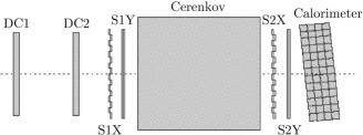
The detector package is enclosed within a concrete shielding hut and includes two drift chambers, two sets of hodoscopes, a gas Čerenkov counter, and a lead-glass calorimeter. A schematic diagram depicting the ordering of the detector package elements is shown in Fig. 2.
Drift chambers
The two multiwire drift chambers baker95 , used for tracking, each consist of six wire planes: (1) the and planes, which provide position information on the -coordinate (dispersive direction); (2) the and planes, which provide position information on the -coordinate (non-dispersive direction); and (3) the and planes, which are inclined at angles relative to the orientation of the and planes. As seen by incoming particles, the ordering of these planes is . The active area of each plane is 113 () 52 () cm2 with an alternating sequence of anode wires (25 m gold-plated tungsten) and cathode wires (150 m gold-plated copper-beryllium) spaced cm apart. The individual wire planes are separated by 1.8 cm, and the two drift chambers are separated by 81.2 cm. The chambers were filled with equal mixtures (by weight) of argon and ethane and maintained at a pressure slightly above atmospheric pressure. The signals from the anodes were read out in groups of 16 by multi-hit time-to-digital convertors (TDCs). The fast branch of the signals from the hodoscope TDCs (to be described shortly) defined the TDC start for the electron arm trigger, while the delayed signals from the drift chamber TDCs formed the TDC stop.
Hodoscopes
The - (-) planes of the two hodoscopes, denoted S1X/S2X (S1Y/S2Y), consist of 16 (10) 75.5-cm (120.5-cm) long Bicron BC404 plastic scintillator bars with a thickness of 1.0 cm and width of 8.0 cm. UVT lucite light guides and Philips XP2282B photomultiplier tubes (PMTs) are coupled to both ends of each scintillator bar. The S1X/S1Y and S2X/S2Y planes are separated by m. The fast branch of the PMT signals was routed to leading-edge discriminators. The discriminated signals were then split, with one set of outputs directed to logic delay modules, TDCs, and scalers, and the other set directed to a logic module. The overall logic signaling a hit in any one of the hodoscope planes required a signal above threshold in at least one of the 16 (10) PMTs mounted on the () side of the bars and at least one of the 16 (10) PMTs mounted on the opposite () side. The slow branch of the PMT signals was directed to analog-to-digital convertors (ADCs).
Čerenkov detector
The Čerenkov detector is a cylindrical tank (165-cm length and 150-cm inner diameter) filled with Perfluorobutane (C4F10, index of refraction at STP). The pressure and temperature in the tank were monitored on an (approximately) daily basis and were observed to be highly stable. Pressures were typically 0.401–0.415 atm (indices of refraction 1.00057–1.00059), translating into energy thresholds of MeV ( GeV) for pions (electrons). The tank is viewed by two mirrors, located at the rear of the tank, which focus the resulting Čerenkov light into two Burle 8854 PMTs. The signals from these PMTs were directed to ADCs. During this experiment, information from the Čerenkov detector was used only for electron-hadron discrimination and not for HMS trigger logic purposes.
Lead-glass calorimeter
The calorimeter consists of 52 TF1 lead-glass blocks stacked into four vertical layers of 13 blocks each. Each block has dimensions of cm3, corresponding to 16 radiation lengths for the total four-layer-thickness of 40 cm. As is indicated in Fig. 2, the four layers of the calorimeter are tilted at an angle of relative to the central axis of the detector package to eliminate losses in the gaps between the individual blocks. Philips XP3462B PMTs are coupled to one end of each block, and the signals from these PMTs were routed to ADCs. Again, information from the lead-glass calorimeter was not used for HMS trigger logic purposes during this experiment.
IV NEUTRON POLARIMETER
IV.1 Overview
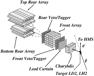
A schematic diagram of the experimental arrangement with an isometric view of the neutron polarimeter is shown in Fig. 3. The first element in the NPOL flight path was a dipole magnet (Charybdis) with a vertically oriented field that was used to precess the neutrons’ spins through an angle in a horizontal plane. As a by-product, protons and other charged particles were swept from the acceptance during asymmetry measurements conducted with the field energized. The next item in the flight path was a 10.16-cm thick lead curtain, located directly in front of a steel collimator (not shown in this figure). The lead curtain served to attenuate the flux of electromagnetic radiation and to degrade in energy the flux of charged particles incident on the polarimeter’s detectors.
The polarimeter consisted of 70 plastic scintillation detectors enclosed within a steel and concrete shielding hut. The front array of the polarimeter functioned as the polarization analyzer (via spin-dependent scattering from unpolarized protons in hydrogen and carbon nuclei), while the top and bottom rear arrays, shielded by the collimator from a direct line-of-sight to the target, were configured for sensitivity to an up-down scattering asymmetry proportional to the projection of the recoil polarization on a horizontally-oriented “sideways” axis (see next subsection). Double layers of thin-width “veto/tagger” detectors located directly ahead of and behind the front array tagged incoming and scattered charged particles. The flight path from the center of the target to the center of the front array was 7.0 m, and the distance from the center of the front array to the center of the rear array (along the polarimeter’s central axis) was m.
IV.2 Polarimetry
IV.2.1 Coordinate systems
Here we establish some necessary notation for a number of different coordinate systems to which we will refer throughout the remainder of this paper.
First, calculations of recoil polarization for the quasielastic 2HH reaction are usually referred to a reaction basis, defined on an event-by-event basis in the - c.m. frame according to
| (6) |
where and denote, respectively, the incident neutron’s momentum and the momentum transfer in the - c.m. frame. The reaction basis can best be visualized by referring to the schematic diagram of the kinematics in the - c.m. frame shown in Fig. 30 of Appendix A.
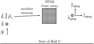
Second, we define a polarimeter basis, , fixed for all events, defined in the laboratory frame according to
| (7a) | |||||
| (7b) | |||||
| (7c) | |||||
with the center of the target defined to be the origin of this coordinate system.
Third, the symmetric geometric configuration of the polarimeter’s top/bottom rear arrays suggests the introduction of a polarimeter momentum basis, , which we again define on an event-by-event basis in the laboratory frame according to
| (8) |
where denotes a unit vector along the incident neutron’s momentum in the laboratory frame. We will henceforth refer to the and axes as the polarimeter’s “sideways” and “longitudinal” axes of sensitivity, respectively. We express the recoil polarization in terms of the polarimeter momentum basis as .
A schematic diagram showing the orientation of the polarimeter basis and polarimeter momentum basis coordinate systems is shown in Fig. 4.
IV.2.2 Detected scattering asymmetry
We define NPOL polar and azimuthal scattering angles, denoted and , according to
| (9a) | |||||
| (9b) | |||||
where is a unit vector along the scattered neutron’s three-momentum, and the unit vector is defined according to .
The cross section for elastic polarized-nucleon, unpolarized-nucleon scattering, denoted for short, is of the form wolfenstein52
where and denote the unpolarized cross section and the analyzing power, respectively. The above approximation is valid in the limit that is small. It is then clear that the asymmetry, , between scattering “up” () and scattering “down” () into infinitesimal solid angles and , respectively, for a particular value of is
| (11) | |||||
A single value of is not, of course, presented to the polarimeter. Also, the top and and bottom rear arrays have a finite geometry; therefore, if the polarimeter is geometrically symmetric in (i.e., geometrically symmetric top and bottom rear arrays), the detected scattering asymmetry (i.e., averaged over kinematics and the top/bottom finite geometry), , is
| (12) |
where and denote, respectively, the acceptance-averaged value of the sideways component of the polarization and the polarimeter’s effective analyzing power averaged over its geometric acceptance (i.e., over ). Henceforth, when we refer to the analyzing power , it should be understood that we are referring to .
IV.3 Charybdis dipole magnet and spin precession
The Charybdis magnet was a water-cooled, 38-ton, 1.5-m tall, 2.3-m wide, and 1.7-m long iron dipole magnet installed in Hall C specifically for this experiment. The magnet was configured such that the gap between the pole pieces was 8.25 inches, and the geometric center of the magnet was located a distance of 2.107 m from the center of the target. The two poles were wired in parallel and powered with a 160 V-1000 A power supply. Two-inch thick iron field clamps with apertures machined to match the 8.25-inch pole gap were placed at the entrance and exit apertures resulting in an effective magnetic length of m.
Calculations of the Charybdis field profile were performed with the TOSCA program tosca for various currents, and values for the field integral, , along the central axis were derived from these calculations. The currents were tuned for the various spin precession angles, , according to the relation
| (13) |
where is the nuclear magneton, for the neutron, and denotes the neutron’s velocity. The field integrals for the precession angles at each of our points are tabulated in Table 3.
| Central | Precession | ||
|---|---|---|---|
| (GeV/) | Angle | [T-m] | |
| 0.447 | 0.604 | 0.6884 | |
| 1.136 | 0.794 | 2.0394 | |
| 1.169 | 0.799 | 0.9123 | |
| 1.474 | 0.839 | 0.9576 | |
| 1.474 | 0.839 | 2.1547 |
The field along the central axis was mapped charybdis at the conclusion of the experiment. We found that the values for the field integrals derived from our mapping results and the TOSCA calculations agreed to better than 0.76% for precession at (GeV/)2, 0.21% for precession at (GeV/)2, and 0.35% for precession at (GeV/)2. Small differences in the measured field integrals for the two magnet polarities (corresponding to a spread) were observed for precession at (GeV/)2. Although we did not conduct field measurements for both polarities at the other points, it is reasonable to assume that the magnet behaved similarly for other current settings.
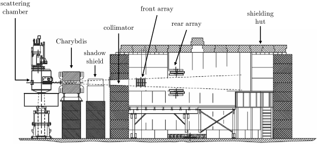
IV.4 Neutron polarimeter physical acceptance
The physical acceptance of the polarimeter was defined by a steel collimator with entrance and exit apertures located 483.92 cm and 616.00 cm, respectively, from the center of the target. The collimator was tapered, with the entrance (exit) port spanning a width of 72.6 cm (92.4 cm) and a height of 37.3 cm (47.5 cm). The 10.16-cm thick lead curtain was located immediately upstream of the collimator’s entrance port.
A schematic diagram of the polarimeter’s shielding hut showing the shielding of the rear array detectors by the collimator from a direct line-of-sight to the target appears in Fig. 5.

IV.5 Neutron polarimeter detectors
The polarimeter consisted of a total of 70 mean-timed BICRON-400 plastic scintillation detectors subdivided into a front veto/tagger array, a front array, a rear veto/tagger array, and symmetric top and bottom rear arrays. The front wall of the polarimeter’s shielding hut was composed of 132.08-cm thick steel blocks; the only opening in this wall was the lead-shielded collimator. A schematic diagram of the polarimeter’s detector configuration is shown in Fig. 6.
IV.5.1 Front veto/tagger array
The function of the first series of detectors in the neutron flight path, the front veto/tagger array, was to identify charged particles incident on the polarimeter. This veto array consisted of two vertically-stacked layers of five cm3 scintillators stacked with their long (160.0 cm) axes oriented horizontally and perpendicular to the central flight path and the thin (0.635 cm) dimension oriented along the flight path. The vertical spacing between the detectors in each layer was mm; therefore, to eliminate charged particle leakage, the two layers were offset from each other in the vertical direction by cm. Each scintillator bar was coupled to two Philips XP2262 2-inch PMTs via plexiglass light guides.
IV.5.2 Front array
The front array was segmented into 20 cm3 scintillators; segmentation of the front array permitted us to run with luminosities as high as cm-2 s-1 (70 A current on a 15-cm liquid deuterium target). The long (100 cm) axes of these detectors were oriented horizontally and perpendicular to the central flight path and were stacked vertically into four layers of five detectors. The long ends of each scintillator were coupled via plexiglass light guides to 2-inch Hamamatsu R1828-01 PMTs powered by bases designed specifically for this experiment for purposes of high gain and highly linear output under conditions of high rate madey83 .
IV.5.3 Rear veto/tagger array
Similar to the front veto/tagger array, the purpose of the rear veto/tagger array was to identify charged particles (e.g., recoil protons from interactions in the front array) exiting the front array. The detectors in this array were identical to those in the front veto/tagger array and were vertically stacked in a similar fashion into two layers of eight detectors each. [We note that only one layer of eight detectors existed for the early part of the experiment during our (GeV/)2 run).] As in the front veto/tagger array, each scintillator was coupled to two 2-inch Philips XP2262 PMTs.
IV.5.4 Rear array
The top and bottom rear arrays each consisted of twelve detectors stacked into three layers of four detectors each. Each layer contained two “10-inch” cm3 detectors sandwiched in between two larger “20-inch” cm3 detectors. These detectors were oriented with their long (101.6 cm) axes parallel to the central flight path and their 50.8 cm or 25.4 cm dimensions oriented horizontally. The centers of the inner, middle, and outer layers were located a vertical distance of 56.72 cm, 73.23 cm, and 89.74 cm, respectively, above or below the central axis of the polarimeter and a horizontal distance of 2.52 m, 2.57 m, and 2.52 m, respectively, from the front array geometric center (see Fig. 6). The long ends of each scintillator were coupled via plexiglass light guides to 5-inch Hamamatsu R1250 PMTs powered by the same bases built for the front array.
The vertical positions of the top and bottom arrays relative to the polarimeter’s central axis were optimized for front-to-rear scattering angles near the peak of the analyzing power for scattering (–20∘ for our range of neutron energies). This configuration with scattering angles in the vicinity of –20∘ also guaranteed, for our kinematics, that only one of the nucleons (for elastic interactions in the front array and assuming straight-line trajectories for the recoil proton through the front array) scattered into either the top or bottom array. We also note that the horizontal position of the middle detector plane was staggered relative to those of the inner and outer layers so that the majority of the front-to-rear tracks passed through at least two of the three horizontal planes, reducing the dependence of the rear array detection efficiency on the scattering angle.
IV.6 Electronics, event logic, and data acquisition
IV.6.1 Electronics
The signals from the 140 NPOL PMTs were processed with electronics sited in two locations: (1) one set, located inside the shielding hut was used to form the timing logic signal for each PMT (past experience with neutron time-of-flight and polarimetry experiments eden94nim revealed that locating the discriminators as close to the PMTs as practical yielded the best timing resolution); and (2) another set, located in the counting house, was used to define the logic for the various event types.
A schematic diagram of the configuration of the electronics in the shielding hut for each scintillator bar in the front and rear arrays is shown in Fig. 7. High voltage was applied to each PMT remotely by an EPICS-controlled 64-channel high-voltage CAEN mainframe crate located in the counting house. Modest levels of high voltage were applied to the PMTs for the front array detectors, as deterioration in the performance of these PMTs was of concern because of the high count rates in these scintillators; however, no deterioriation in their performance was observed during the experiment (instead, gains were stable to within %). To compensate for the resulting lower levels of gain obtained directly from these PMTs, the anode signals were preamplified by fast preamplifiers with a gain of eight, custom-designed and assembled for this experiment. The anode signals from the PMTs in the rear array and the front and rear veto/tagger arrays were not preamplified.
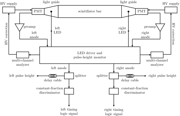
The anode signals from the front and rear arrays were then directed to an LED driver and pulse height monitor. When desired, this device was used to assess the response of each PMT to a flashing blue LED mounted on its light guide. The centroid channels of the LED spectra were monitored periodically, and any necessary changes to the high voltage levels were performed remotely. The gains of the front and rear veto/tagger array PMTs were not monitored with this system.
The anode signals from all four detector arrays were then split. The signals in the fast branch (for the event trigger and timing measurements) were directed to either constant-fraction discriminators (front and rear arrays) or leading-edge discriminators (front and rear veto/tagger arrays) located inside the shielding hut and then sent to the electronics in the counting house. We did not employ constant-fraction discrimination for the veto/tagger array detectors for the following reasons: (1) the dynamic range of energy deposition in these detectors was small for those events of interest, so the time-walk was tolerable; and (2) the timing measurements from these detectors were not used for energy determinations, so resolutions of a few ns were sufficient for charged particle tagging. Those signals diverted to the slow branch were routed through delays located inside the shielding hut and then sent to the counting house.
Upon arrival in the counting house, both the analog and timing signals were directed through filters/transformers designed to eliminate low-frequency noise. The analog signals were then sent directly to ADCs, while the timing signals were first sent to discriminators and then routed to two branches of a timing circuit. In one branch, the output from these discriminators were directed through level translators, delays, discriminators, and then further split and directed to TDCs and scalers. In the other branch of this timing circuit (used to form the event triggers), the timing signals from the PMTs on all of the detectors, except those in the rear veto/tagger array, were first sent to logic modules which were used to generate logic signals for coincidences between the timing signals for the two PMTs on each detector. Logical ORs were generated for each of the twenty front array detector two-PMT coincidences. These signals were then sent to a fan-in with one set of outputs directed to scalers and the other through a discriminator; the output from this discriminator was then directed to the trigger circuit. The logical ORs for the rear array detectors and the front veto/tagger-array detectors were routed through a fan-in and then directed to the trigger circuit. The timing signals from the rear veto/tagger-array detectors were not used for trigger purposes.
IV.6.2 Event logic and triggers
All event trigger logic was performed by two LeCroy 8LM 2365 Octal Logic Matrix modules. Pretrigger logic signals from the HMS (coincident hits in at least three of the four hodoscope planes), the NPOL front array, the NPOL rear array, and the NPOL front veto/tagger array were routed to the 8LM modules. In addition to these logic signals, triggers from the polarized electron source were also input to these modules. As previously discussed, the helicity of the electron beam was flipped pseudorandomly at 30 Hz. Electronics at the polarized source generated a logic signal for readout of helicity-gated scalers for each 33.3 ms helicity window. Further, these modules also generated a helicity-transition logic signal which was used to veto otherwise valid data triggers that occured during transitions at the polarized source from one helicity state to another. The duration of this helicity-transition logic pulse was s, resulting in an effective data-taking helicity window of ms.
An electronic module known as the Trigger Supervisor (TS) functioned as the interface between the 8LM logic modules and the data acquisition system (DAQ). The TS generated a logic signal indicating the status of the DAQ (e.g., busy or not busy) that was input to the logic modules. The logic modules then determined whether the logic for any of the eight possible physics triggers (e.g., electron singles, electron/front array coincidences, electron/front array/rear array coincidences, etc.) was satisfied. If the logic for any particular trigger was satisfied, the TS generated an accept signal leading to generation of the appropriate ADC gate and TDC common signals. The ADCs, TDCs, and scalers were then read out with real-time UNIX-based processors.
The event triggers of interest were three-fold coincidences between hits in the electron arm, the front array, and the rear array. These events constituted –85% of the event triggers, as the higher rate events, such as electron singles or two-fold coincidences between the electron arm and the front array, were prescaled.
IV.6.3 Data acquisition
The DAQ was controlled by the CEBAF Online Data Acquisition System (CODA) jlabcoda . CODA includes an event-builder subsystem programmed to assemble the individual ADC channel, TDC channel, and scaler read-out data fragments into an event. The data for the events were then written to disk in CODA format by another subsystem.
Typical data acquisition rates were one million events in () hours with the Charybdis dipole field energized (de-energized).
V Data analysis
V.1 Electron reconstruction and tracking
V.1.1 Overview of analysis code
The raw ADC, TDC, and scaler data written to disk and encoded by the DAQ in CODA format were decoded with a modified version of the standard Hall C ENGINE analysis code (see, e.g., arrington98 for a discussion of the standard version) employed for the analysis of nearly all experiments conducted in Hall C. Modifications to the standard version were necessary to accommodate the raw data stream from the 70 NPOL detectors; hereafter, whenever we refer to the ENGINE analysis code, it should be assumed that we are referring to our modified version of this code.
For each event, the scattered electron’s track through the HMS was reconstructed, and various kinematic quantities (e.g., momentum, energy, focal plane distributions, etc.) were computed. ENGINE was not configured to reconstruct the track of the nucleon through the polarimeter; instead, the NPOL detector data were simply written to new data files for later processing by other analysis tools.
V.1.2 Extraction of electron information
Tracking
The overall strategy of the tracking algorithm arrington98 was to use the hit information from the drift chambers and reference start times provided by TDC information from the scintillators in the hodoscope planes to reconstruct the trajectory of the particle through the drift chambers. TDC information from those scintillators in the hodoscope planes recording hits was used to establish reference start times. This information, coupled with TDC information from the drift chambers, was then used to determine the location of the hit in the drift chamber planes. “Left-right ambiguities” in the drift chambers (i.e., whether a particle passed to the left or right of any given wire) were resolved by fitting a (straight-line) track to each left-right hit combination in the six planes of each drift chamber. The full track through both drift chambers with the overall smallest track reconstruction was defined to be the final reconstructed track through the drift chamber planes.

Transport
ENGINE then attempted to relate the positions and angles at the focal plane (determined from the track through the drift chambers) to target quantities. In standard coordinate notation for transport through a spectrometer, is taken to point along the central ray of the spectrometer, in the dispersive direction (by convention, taken to point “downwards”), and . It should be noted that HMS focal plane variables are traditionally referred to the detector focal plane, defined to be perpendicular to the central ray (i.e., parallel to the drift chamber planes) with the origin of the - plane defined to be that point in space where the central ray of the spectrometer intersects the true (magnetic) focal plane. In addition to the dispersive and non-dispersive variables, two other standard transport variables, and , are defined to be the slopes of the rays at the focal plane, and , respectively. The focal plane variables , , , and were converted to target quantities , , , and , where denotes the central momentum setting, via computation of transport matrix elements derived from optics studies. For this choice of target coordinates, was not reconstructed but was, instead, defined to be for all events.
V.1.3 Sample electron reconstruction results
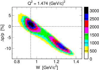
Sample histograms of the reconstructed -distribution, hereafter referred to as the “-distribution”, at our lowest and highest points are shown in Fig. 8. The quasielastic peak is clearly visible in both spectra, but a large accompanying background of inelastic events associated with pion-production in the target is present in the (GeV/)2 spectrum. Inelastic peaks were also clearly visible in the and 1.169 (GeV/)2 spectra but are not shown here. A sample two-dimensional histogram of plotted versus the invariant mass, , calculated from the electron kinematics according to
| (14) |
where is the nucleon mass, is shown in Fig. 9 for our (GeV/)2 point. The resonance is prominent in this distribution.
Hadrons in the HMS were identified via examination of the Čerenkov photoelectron spectrum. As expected, a hadron peak was not visible in the (GeV/)2 spectrum; however, prominent hadron peaks (at zero photoelectrons) were observed at the three higher settings. An example of such a photoelectron spectrum from our (GeV/)2 data is shown in Fig. 10. Cuts on the number of photoelectrons, coupled with cuts on the energy deposition in the calorimeter, were sufficient for electron-hadron discrimination.

V.2 Neutron polarimeter energy calibration
The (charge-integrating) ADCs for the front and rear array detector PMTs were calibrated with the Compton spectra from a 228Th source (2.61 MeV -rays); the front and rear veto/tagger array detectors were not calibrated as ADC information was not used for charged particle tagging. These calibrations were parametrized in terms of an equivalent electron energy (denoted “eVee”), where the relation between the light output of recoil protons and Compton-scattered electrons in organic scintillator was found by Madey et al. madey78 to be well described by the parametrization
| (15) |
Here, denotes the energy deposition of a recoil proton, denotes the energy deposition of an electron that yields the equivalent light output, and the are empirically determined parameters.
Unfortunately, the range of electron energies (2.38 MeV Compton edge) was not sufficient, as typical energy depositions for the recoil protons were estimated to be several MeVee plaster03 ; further, the hardware thresholds for the front (rear) array detectors were set at 4 (10) MeVee. To remedy these shortcomings, a custom-designed linear amplifier with a gain of ten was placed in the timing circuit during calibration runs. The resulting ADC spectra were fitted to the sum of the Klein-Nishina distribution (smeared by a Gaussian resolution function) and an exponential background tail. Pulse-height calibrations were performed at three different times during the experiment (roughly at the start, middle, and conclusion); minor differences (%) in the extracted calibration parameters were observed but were deemed to be relatively unimportant as the selection of quasielastic 2HH events did not rely heavily on pulse height information.
V.3 Neutron polarimeter timing calibration
To optimize track reconstruction and background rejection in the neutron polarimeter, the relative timing relationships between the NPOL detectors and the HMS were carefully calibrated with a series of algorithms designed to: (1) generate position calibrations for each detector; (2) generate relative timing calibrations for each detector in the front array and discern the relationship between the mean time for each front array detector and the trigger mean time; (3) calibrate the timing between the HMS and the front array (yielding a coincidence time-of-flight); (4) generate relative timing calibrations for each detector in the rear array and calibrate the time-of-flight between the front array and the rear array; and (5) generate position and timing calibrations for the front and rear veto/tagger detectors.
V.3.1 Front and rear array position calibrations
The position calibration algorithm for the front and rear array detectors employed data acquired with the Charybdis magnet de-energized, such that charged particles illuminated the front array almost uniformly. The relationship between the hit position and the difference (in channels) between the TDCs from the PMTs mounted on the two ends of each scintillator was parametrized in a linear form with an unknown slope and offset. Histograms of these TDC channel differences were accumulated for each detector and then boxcar-smoothed. The algorithm identified the channel of maximum content and then scanned away in both directions until channels with 10% of the maximum content were identified. Slope and offset parameters were then chosen such that these 10%-content channels were aligned with the physical edges of each detector; the resulting calibrated position spectra displayed sharp edges near the physical detector edges.
V.3.2 Front-array timing and trigger calibrations
The first goal of the front-array timing calibration was to align the mean times of all the detectors in the front array using events with a single hit in the front array. Data acquired with the Charybdis magnet energized (for suppression of background processes) were employed for this step of the timing calibration, and events with () hits in the front veto/tagger array (front array) were discarded. An offset was chosen for each detector such that the mean value of its mean-time spectrum was aligned on zero.
The second goal of the front array timing calibration was to construct a variable that could be used to identify which hit generated the trigger (for events with multiple front array hits), as the trigger circuit did not identify the triggering hit. Proper identification of the triggering hit via examination of the correlation between the TDC channels for the two PMTs on each detector and the position dependence of the mean times yielded self-timing spectra with FWHM of ns.
V.3.3 Coincidence time-of-flight calibrations
To maximize our signal-to-noise ratio, we constructed a coincidence time-of-flight variable that accounted for the quasielastic 2HH kinematics, pathlength variations through the HMS and NPOL, and variations in the delay between an interaction in a detector and the arrival of its timing signal at the TDC. For this step of the calibration, a minimal set of cuts were applied to the data for purposes of (loose) quasielastic event selection (e.g., cuts on the calorimeter energy deposition, , etc.). Again, front array single-hit events (with no hits in the front veto/tagger array) acquired with the Charybdis magnet energized were used for this step of the calibration.
The algorithm first predicted the neutron time-of-flight from the target to the front array using only position information (i.e., the reconstructed vertex information for the primary scattering event in the target cell and the position of the front array hit) and electron kinematics. For a three-body final state (i.e., no pion production), four-momentum conservation demands
| (16a) | |||||
| (16b) | |||||
From this, it follows that a value for (and, then, the predicted neutron time-of-flight) can be derived from the solution to the quadratic equation , where
| (17a) | |||||
| (17b) | |||||
| (17c) | |||||
| (17d) | |||||
A value for the actual measured time-of-flight was then extracted from information in the signal output of a TDC started by a signal generated by the NPOL trigger and stopped by the HMS trigger, a correction for pathlength variations and delays between interactions and signals in the HMS computed by ENGINE, and the mean time of the front array detector recording the hit. This measured time-of-flight was then compared with the predicted time-of-flight, and the resulting difference, the coincidence time-of-flight (hereafter, referred to as cTOF), was computed for each event. The resulting cTOF spectra were fairly narrow with FWHM of ns and signal-to-noise ratios of :1–10:1. Sample cTOF spectra are shown later in this paper.
V.3.4 Rear-array timing calibrations
The algorithm for the rear-array timing calibration selected single-hit events (with no hits in both the front and rear veto/tagger arrays) acquired with the Charybdis magnet energized and then filtered these hits according to a set of cuts designed to select quasielastic events. In addition, a ns cut was enforced.
In the first step, the algorithm aligned the mean time spectra of the rear array detectors relative to each other. As for the front array, histograms of mean times were accumulated for each detector. The channel of maximum content was identified, and an offset parameter for each detector was then chosen such that the peak channel was aligned on zero.
In the second step, the algorithm performed an absolute timing calibration of the rear array detectors relative to the front array detectors via a front-to-rear velocity calibration. The scattering angle for the front-to-rear track was computed using the incident neutron’s three-momentum and the position information for the hits in the front and rear array. The algorithm then predicted the front-to-rear velocity for elastic scattering in the front array via computation of the scattered neutron’s kinetic energy, , where
| (18) |
Here, denotes the incident neutron’s kinetic energy, denotes the neutron scattering angle in the polarimeter, is the usual Lorentz factor for the incident neutron, and the proton and neutron masses are assumed to be equal. Relative time-of-flight (hereafter, referred to as rTOF) histograms, defined to be the difference between the predicted and measured values of the front-to-rear time-of-flight, were accumulated, and offsets were then chosen for each detector such that the peak channel was aligned on zero. Again, sample rTOF spectra are shown later in this paper.
V.3.5 Front and rear veto/tagger-array calibrations
The position and timing calibration of the front and rear veto/tagger-array detectors consisted of three steps. Data for charged particle tracks acquired with the Charybdis magnet de-energized were employed for this calibration; hits were required in each layer of the front veto/tagger array, the front array, and the rear veto/tagger array.
First, as leading-edge discrimination was employed for these detectors, the algorithm began by computing corrections for walk. The relationship between the observed TDC and ADC channels, and , was parametrized as , where TDC denotes the TDC channel in the absence of walk effects, is an empirical parameter, and denotes the peak ADC channel. A value for was then computed via the method of least squares.
Second, the veto/tagger array detectors were position calibrated using a different algorithm than that employed for the position calibration of the front and rear array detectors due to the facts that the collimator partly obscured the edges of the front veto/tagger array detectors and that the outer rear veto/tagger array detectors did not receive adequate illumination from front-to-rear charged tracks. (The front and rear veto/tagger arrays were designed to provide more than adequate coverage of target-to-front and front-to-rear charged tracks.) As such, position calibration parameters for these detectors were deduced via a comparison of the recorded hit position with the nearest hit position in the front array, and offset parameters were determined via a minimization of the difference between the predicted and recorded hit positions. To improve the statistics for the outer rear array veto/tagger detectors, the algorithm searched for charge-exchange events in the front array. Tracks from these events were used to predict hit locations in the rear veto/tagger array detectors, and position calibration parameters were then deduced from another minimization of the difference between the predicted and recorded hit positions. The resulting calibrated position spectra were well aligned about the physical center of each detector with somewhat more rounded spectra than observed in the front and rear array spectra due to the use of leading-edge discrimination.
Last, the mean times were aligned relative to each other via the same procedure employed for the mean-time calibration of all the other detectors.
V.4 Nucleon reconstruction and tracking

V.4.1 Overview of analysis code
The algorithm we developed for reconstruction and tracking in the neutron polarimeter began by translating the raw NPOL detector data decoded by ENGINE into hit positions and times. The code then attempted to determine which hit in the front array generated the trigger. All hits were then filtered according to a number of different selection criteria, with the surviving hits grouped into recognizable patterns. The code then attempted to determine the primary hits in the front and rear arrays and the charges of the incident particle and the particle detected in the rear array. Finally, kinematic quantities and time-of-flight variables were then computed for those events satisfying all tracking criteria.
V.4.2 Trigger selection and hit filtering
The algorithm assigned the location of the triggering front array hit to the detector with the smallest absolute self timing value. All hits were then filtered according to a number of selection criteria designed to discard hits with unphysical reconstructed detector positions or mean times falling outside of specified windows. These mean time windows were chosen sufficiently wide for purposes of quasielastic event selection, elastic/quasielastic scattering in the front array, and charged particle tagging in the veto/tagger arrays. In particular, the mean-time windows for both the front and rear veto/tagger arrays safely bracketed the entire peak regions with the borders extending into the regions of flat background.
V.4.3 Pattern grouping and track reconstruction
Incomplete and simple events
The algorithm began by identifying incomplete and simple events. First, events with either no surviving hits in the front and/or rear array or events with hits in both the top and bottom rear array were discarded. Second, simple events with exactly one hit in the front array, one hit in the rear array, and no hits in both the front and rear veto/tagger arrays were identified. For these events, the incident particle and the particle detected in the rear array were, obviously, designated neutral particles, and reconstruction of the track was deemed complete.
Multiple hit events
The majority of the events were more complicated than these simple events because of propagation of the recoil protons through adjacent scintillator bars or multiple scattering of the neutron. For these more complicated events, the code began by identifying which layer in the front array (i.e., first, second, third, or fourth) was hit first; henceforth, we will refer to the hit(s) in this layer as the “first cluster”. If the first cluster contained more than one hit, the (vertically) highest and lowest hits were identified; such hit patterns were assumed to be the result of an or interaction in one detector followed by the penetration of the recoil proton into a vertically adjacent detector. Accordingly, if the hits occurred in non-contiguous detectors within the same vertical layer (i.e., existence of a vertical “gap”), the event was discarded.
The code then searched for evidence of one or more “missing layers” in the front array (e.g., an event with hits in the first layer and the fourth layer); a missing layer was taken to be evidence for multiple scattering of the incident neutron. If such a “second cluster” of hits was not found, the location of the front array scattering vertex was assigned to the highest (lowest) hit in the first cluster if the top (bottom) rear array recorded one or more hits. If, instead, a second cluster of hits was found, the code determined whether the second cluster contained a gap; again, events with gaps in the second cluster were discarded. The algorithm then attempted to discern whether the second cluster was located above or below the first cluster; if the second cluster was above (below) the first cluster, the location of the first cluster scattering vertex was assigned to the highest (lowest) hit in the first cluster. Then, if the top (bottom) rear array was hit, the location of the second cluster scattering vertex was assigned to the highest (lowest) hit in the second cluster. Finally, if more than one hit was recorded in either the top or bottom rear array, the rear array scattering vertex was assigned to that hit closest in distance to the final front array scattering vertex.
V.4.4 Charge identification
After the track through the front and rear arrays was reconstructed, the code then checked for hits in the veto/tagger arrays. The charge of the incident particle was determined via the following algorithm. (1) If there were no hits in any of the front veto/tagger detectors, the particle was designated a neutral particle. (2) If there were hits in the front veto/tagger detectors, the radial distance between the location of the veto/tagger hit and the location of the first scattering vertex was computed according to , where the coordinates refer to the polarimeter basis, defined in Eq. (7). If at least one hit in each veto/tagger layer satisfied cm, the incident particle was designated a charged particle. If no hits in either veto/tagger layer satisfied cm, the incident particle was designated a neutral particle. Finally, if a hit in one of the front/veto tagger layers satisfied this distance requirement but no hits in the other layer satisfied this condition, the charge of the incident particle was declared to be ambiguous.
The algorithm for the determination of the charge of the particle detected in the rear array was essentially identical to that described above. The only difference was that the code predicted where the hits in the rear veto/tagger arrays should have occurred assuming a straight-line trajectory from the final front array scattering vertex to the rear array scattering vertex. The computed value of the radial distance between the location of the actual hit and the predicted hit was then used, in an identical manner, for rear array neutral/charged tagging.
The choice of the 30-cm radial track-distance threshold was based on an examination of track-distance spectra for the front and rear veto/tagger arrays. The spectra for the front veto/tagger array were found to be relatively narrow with an abrupt change in slope around 30 cm, believed to be related to these scintillators’ position resolution. The spectra for the rear veto/tagger array did not contain such a feature as the recoil protons arising from interactions in the front array were widely distributed in angle; nevertheless, the same 30-cm condition was employed as the position resolutions for these detectors were similar to those in the front veto/tagger array.
V.4.5 Kinematic distributions and time-of-flight variables
Following reconstruction of the track through the polarimeter, kinematic and time-of-flight quantities were computed for fully reconstructed events. First, the incident particle’s momentum was computed using only position information for the reconstructed target vertex, position information for the first scattering vertex in the front array, and the four-momentum transfer , via solution of the quadratic equation for given previously in Eq. (17). The momentum was then used to predict the target-to-front array time-of-flight; the difference between the predicted and measured time-of-flight was then stored as the cTOF variable. Laboratory frame polar and azimuthal neutron scattering angles with respect to , and , were computed from information on and . Second, front-to-rear polar and azimuthal scattering angles, and , were computed using information on and the scattering vertices in the front and rear arrays. This information was used to compute a value for , Eq. (18), which was then used to predict the front-to-rear time-of-flight; the difference between the predicted and measured time-of-flight was then stored as the rTOF variable. Finally, the missing momentum, , missing energy, , and missing mass, , were computed according to
| (19a) | |||||
| (19b) | |||||
| (19c) | |||||
V.4.6 Sample nucleon reconstruction results
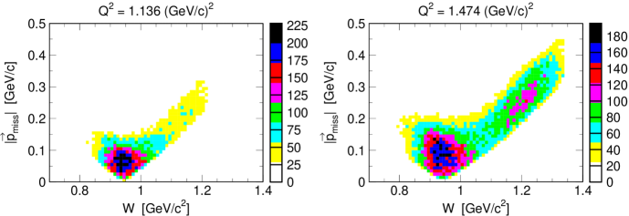
To illustrate the full range of the polarimeter’s acceptance, sample two-dimensional histograms of plotted versus the invariant mass at our and 1.474 (GeV/)2 points are shown in Fig. 12. A minimal set of cuts designed to eliminate scattering from the target cell walls, hadrons in the HMS, and protons incident on NPOL were applied to these spectra. Our acceptance was sensitive to missing momenta ranging up to MeV/ at our highest point. As can clearly be seen in these correlation plots, quasielastic events were associated with missing momenta in the range MeV/. Larger values of are, of course, seen to correspond to inelastic events, with the resonance prominent at large missing momenta in the (GeV/)2 spectrum. The correlation plot for (GeV/)2 was essentially identical to that at (GeV/)2, while the (GeV/)2 distribution was restricted to considerably smaller ranges of ( MeV/).
V.5 Data selection criteria, data sets, and cuts
V.5.1 Data selection criteria and data sets
Only those data runs satisfying the following criteria were employed for the final production data analysis: (1) no problems with the HMS equipment (e.g., magnet trips, detector failures, etc.); (2) no problems with delivery of the electron beam (e.g., unstable beam parameters); (3) no problems with the DAQ; (4) no problems with the cryogenic target (e.g., large temperature fluctuations, monitoring system failures, etc.); and (5) no problems with the Charybdis magnet or the NPOL detectors (e.g., fluctuations in the magnet current, detector high-voltage trips, etc.). We note that additional problems may have resulted in the designation of a run as unsuitable for the production analysis.
| Central | Precession | Charge |
| (GeV/) | Angle | Coulombs |
| 0.447 | ||
| 0.447 | ||
| 1.136 | ||
| 1.136 | ||
| 1.136 | ||
| 1.169 | ||
| 1.169 | ||
| 1.474 | ||
| 1.474 | ||
| 1.474 | ||
| 1.474 | ||
| 1.474 | ||
| Total |
The quantity of data satisfying the above selection criteria is summarized in Table 4. There, we list the accumulated charge for each of the individual points and neutron spin precession angles.
V.5.2 Cuts for extraction of time-of-flight spectra
A summary of the final set of cuts applied to the production data sets for extraction of the cTOF and rTOF time-of-flight spectra is as follows.
Target variables
Scattering from the target cell windows was suppresed via the requirement that the reconstructed target vertex lie within cm of the center of the target (for the 15-cm target) along the incident beamline. Further, events with unreasonable reconstructed values for and were discarded.
HMS variables
The reconstructed electron track was required to fall within the the collimator acceptance, and events with unreasonably large track reconstruction values were discarded. Hadrons in the HMS were suppressed via cuts on the number of Čerenkov photoelectrons and the energy deposition in the calorimeter. Events away from the quasielastic peak were suppressed via a tight cut.
NPOL variables
Software thresholds of 8 (20) MeVee designed to suppress low-energy backgrounds were applied to the front (rear) array pulse height distributions. Also, to suppress lower-energy neutrons originating from charge-exchange Pb reactions in the lead curtain (discussed in more detail later), the mean times for front array hits were required to lie within a ns window, due to the expected degradation in the energy of the incident protons prior to the charge-exchange reaction. Events with more than one scattering vertex in the front array (i.e., existence of a second cluster) were discarded to eliminate the effects of depolarization following the first interaction in the front array.
The front-to-rear polarimeter scattering angle, , was required to satisfy at (GeV/)2 and for the other points. The lower cut of eliminated unreasonably small scattering angles, while the upper cut of or was used to suppress zero (or negative) values of the analyzing power at larger scattering angles (as predicted by SAID arndt03 ).
reaction variables
Pion-production events were suppressed via tight cuts on the missing momentum and invariant mass of MeV/ and GeV/.
V.6 Extraction of time-of-flight spectra and scattering asymmetries
V.6.1 Polarimeter event types
An analysis code developed to extract the physical scattering asymmetries subjected each event to the cuts discussed previously. In addition, each event was also subjected to a more stringent test for the determination of the incident particle’s charge. As we used single-hit TDCs, an early accidental hit in a front veto/tagger detector falling outside the mean-time window for the front veto/tagger array would have prevented that TDC from recording any later (on-time) hits, leading to the incorrect tagging of a charged particle as a neutral particle.
Histograms of cTOF were accumulated for two types of front array scattering events, and events, corresponding (for a neutral particle incident on the polarimeter) to the detection of a neutral and charged particle, respectively, in the rear array. We identified events with the scattering of the neutron from the front array to the rear array, while we identified events with forward scattering of the recoil proton with sufficient energy for penetration of the front array. It should be noted that for the incident neutron kinetic energies of interest, the analyzing power for elastic scattering becomes negative for neutron scattering angles greater than ; therefore, the signs of the detected asymmetries for and events were the same. Events with charges deemed ambiguous in either the front or rear array were rejected.
Histograms of rTOF summed over all front-to-rear tracks were accumulated for those events falling within a prescribed cTOF window. To compensate for variations in the flight path between the front array and the rear array, the rTOF values were normalized to a nominal 250-cm flight path. The accumulated rTOF spectra were decomposed into the following event types: (1) “RU events” (positive beam helicity and scattering from the front array to the top rear array); (2) “LU events” (negative beam helicity, top rear array); (3) “RD events” (positive beam helicity, bottom rear array); and (4) “LD events” (negative beam helicity, bottom rear array). The scattering asymmetries were then extracted from the yields in these four spectra.
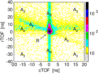
V.6.2 HMS-NPOL coincidence event types
A two-dimensional histogram of the correlation between cTOF and rTOF summed over and events at (GeV/)2 is shown in Fig. 13.

Five different event types can readily be identified in this correlation plot. (1) Real three-fold HMS/front-array/rear-array coincidence events are denoted “” and form the peak centered at ns. (2) Three-fold accidental coincidences, denoted “”, require a random electron in the HMS, a random neutral particle in the front array, and a random particle in the rear array, and are distributed uniformly over the entire plot area. (3) Real two-fold front-array/rear-array coincidences with an accidental electron are denoted “” and are associated with the “horizontal band” defined by ns. (4) Real two-fold electron/front-array coincidences with an accidental rear array particle are denoted “” and are identified with the “vertical band” defined by ns. (5) Real two-fold electron/rear-array coincidences with an accidental front-array particle are denoted “”. These events are located along a diagonal band defined (approximately) by . Such events are attributed to the corruption of an otherwise -type event by an accidental front array hit occuring some time before or after the true interaction. The values of cTOF and rTOF extracted from the data will then be and , where the “uncorr” subscript denotes the (true) uncorrupted values. For uncorrupted values centered on zero, it then follows that , in accordance with the observed result.
V.6.3 Quasielastic event selection

Real -type coincidence events were selected via tight ns and ns cuts. As evidence our cuts selected quasielastic 2HH events, comparisons of invariant mass spectra, , obtained before and after cuts on , , cTOF, and rTOF are shown in Fig. 14 for our and 1.474 (GeV/)2 points. After all cuts (except for the additional cut on GeV/ itself), these distributions converged to fairly narrow peaks centered on the neutron mass.
V.6.4 Extraction of asymmetries from time-of-flight spectra

One-dimensional projections of cTOF are shown in Fig. 15 for our lowest and highest points. Histograms of rTOF were accumulated for those events falling within the ns peak cTOF window. In addition, histograms of rTOF were accumulated also for a sampled background region of ns in the cTOF spectrum. The signal-to-noise ratios were independent of the state of the Charybdis magnet at each of our points.
Sample rTOF spectra summed over all RU, LU, RD, and LD events for cTOF peak events at our lowest and highest points are shown in Fig. 16. The asymmetric tails on the slow sides are due to scattering from protons bound in carbon nuclei and other nuclear reactions, and the small satellite peak observed in the (GeV/)2 spectrum on the fast side at ns is attributed to quasifree -production in the scintillators, followed by decay and detection of a photon in the rear array. Indeed, front-to-rear velocity spectra for these events are centered on . This -production peak was observed in the , 1.169, and 1.474 (GeV/)2 rTOF spectra but was absent in the (GeV/)2 spectrum, as the energies of those neutrons were below threshold.
The yields for those events falling within the ns rTOF window were obtained via peak fitting, with contributions from the -production peak and the flat background excluded. These yields were then further corrected for the contents of the rTOF spectra accumulated for the sampled cTOF background region. The desired quantities, the physical scattering asymmetries, , were extracted from the final background-subtracted yields in the four decomposed rTOF spectra via the cross-ratio technique ohlsen73 . In obvious notation, the cross ratio, , is defined to be the ratio of two geometric means,
| (20) |
and is related to the asymmetry via
| (21) |
The merit of the cross-ratio technique is that is insensitive to ohlsen73 : (1) the number of particles incident on the polarimeter (i.e., target luminosities) for the two beam helicity states; and (2) the relative efficiencies and acceptances of the polarimeter’s top and bottom rear arrays.
V.7 Asymmetry results
V.7.1 Electron beam polarization normalization
Unlike recoil polarization measurements in which both polarization components, and , can be extracted simultaneously from the data (e.g., recoil polarization experiments with focal-plane polarimeters), our polarimeter was sensitive to only one of these components (or a combination thereof). As such, it was necessary to normalize our run-by-run scattering asymmetries to some common value of the beam polarization.
Our normalization procedure was as follows. As the beam polarization was measured only periodically with the Møller polarimeter, we defined the beam polarization for a run to be the result of the most recent prior Møller measurement (if the accelerator parameters were unchanged in the interim). All of our run-by-run scattering asymmetries and their statistical errors were then normalized to a common value of 80%.
We found that the beam polarization was fairly stable, with small (few percent) fluctuations observed in successive measurements during periods of continuous beam delivery to our experiment. To illustrate, the results of 23 successive Møller measurements conducted during our (GeV/)2 running period spanning the days of February 20, 2001 through March 5, 2001 are shown in Fig. 17.

V.7.2 Corrections for charge-exchange in the lead curtain
Contamination from the two-step 2H + Pb charge-exchange reaction in the lead curtain could either dilute the “real” 2H asymmetry or contribute to a false asymmetry if the flux of charge-exchange neutrons was unpolarized or polarized, respectively. A significant advantage of our neutron flight path setup in which the lead curtain was located downstream of the Charybdis dipole field was that the majority of the quasielastic protons were swept from the front face of the lead curtain.
Accounting for such nuclear reactions, the measured asymmetry, , can be parametrized as
| (22) |
where denotes the contamination level from the two-step charge-exchange process, denotes the asymmetry for charge-exchange neutrons, denotes the fraction of 2H neutrons, and denotes the asymmetry for the 2H reaction. The asymmetry for the background process can further be written as
| (23) |
where and denote, respectively, the projections of the 2H recoil proton’s polarization on the polarimeter momentum basis - and -axis; is the proton spin precession angle in the Charybdis field; and denotes the polarization transfer coefficient for the Pb reaction. It then follows that if , , , , , and are all known or measured, can be determined.
To estimate the contamination levels, , we took data with a liquid hydrogen target. The rates for and events extracted from these data were compared with those extracted from our liquid deuterium data and corrected for differences in the two targets’ densities and atomic numbers. We found that the contamination levels were negligible (%) at all of our points when the Charybdis field was energized for and precession and also when the field was de-energized at (GeV/)2 for precession; therefore, we did not apply corrections to any of these asymmetries. Non-negligible event rates were observed when the Charybdis field was de-energized for precession at (GeV/)2, with observed contamination levels of % and % for and events, respectively. Corrections were applied to these asymmetries assuming for our kinematics of MeV. was measured at MeV and found to be consistent with zero () prout00 .
V.7.3 Summary of asymmetry results
Our final asymmetry data for and events at each of our points and precession angles are tabulated in Table 5. To illustrate the quality of our asymmetry data, a histogram of the asymmetries for the (GeV/)2 data set is shown in Fig. 18; the distribution is of an appropriate Gaussian shape.
| Central | Precession | ||
|---|---|---|---|
| (GeV/ | Angle | [%] | [%] |
| 0.447 | |||
| 0.447 | |||
| 1.136 | |||
| 1.136 | |||
| 1.136 | |||
| 1.169 | |||
| 1.169 | |||
| 1.474 | |||
| 1.474 | |||
| 1.474 | |||
| 1.474 | |||
| 1.474 |


V.8 Extraction of uncorrected values for
| Central | [deg] | ||||
|---|---|---|---|---|---|
| (GeV/) | Combined111Weighted average of from and events. | ||||
| 0.447 | |||||
| 1.136/1.169222Result obtained via averaging of the nominal (central) electron kinematics for the two points. | |||||
| 1.474 | |||||
We extracted values for from our asymmetry data assuming elastic scattering from a free neutron and infinitesimal pointlike HMS and NPOL acceptances and neglecting nuclear physics corrections for FSI, MEC, and IC. To do so, we fitted the asymmetries as a function of the precession angle to the functional form , where the phase-shift parameter was defined in terms of form factors and kinematics in Eq. (4). To illustrate the quality of these fits, our (GeV/)2 and asymmetry data are plotted as a function of the precession angle in Fig. 19. These data are fitted well by sinusoids with excellent agreement seen between the independent fits to the and asymmetry data. We could not fit the (GeV/)2 asymmetries to a sinusoid as asymmetry data were taken only at two precession angles.
V.9 Simulation programs
We developed two independent simulation programs, GENGEN and the Acceptance program, to extract acceptance-averaged and nuclear physics corrected values for from our measured experimental asymmetries. The GENGEN simulation program, a pure Monte Carlo simulation program, included realistic models for the primary 2HH reaction in the target, the HMS acceptance, neutron spin precession in the Charybdis dipole field, spin-dependent neutron scattering in the lead curtain, elastic and quasielastic scattering in the front and rear arrays of NPOL, tracking of the incident neutron and recoil proton from the front array to the rear array, and the detector response of the polarimeter to interactions in the front and rear array. The Acceptance program was not a Monte Carlo simulation program, but was, instead, designed to extract the corrections for the finite experimental acceptance and nuclear physics effects directly from our experimental data.
V.9.1 GENGEN simulation program
Event sampling technique
A uniform sampling scheme was employed in which events were generated uniformly over the available kinematic phase space, with an event weight computed according to a model cross section. The vertex position for the primary 2HH interaction in the extended target was sampled uniformly within the raster pattern, and the scattered electron’s kinematics were sampled uniformly over specified ranges. The physical acceptance of the HMS was enforced via inclusion of an HMS transport model taken from the SIMC simulation code simc . In-plane and out-of-plane scattering angles for the recoil neutron were sampled uniformly over specified ranges, permitting computation of the magnitude of the neutron’s momentum according to Eq. (17). Complete specification of the electron and neutron kinematics permitted computation of those variables of particular interest for the quasielastic 2HH reaction, such as , , etc.
Cross section and recoil polarization
We employed the Arenhövel formalism arenhovel87 ; arenhovel88 ; arenhovel95 for computation of the 2HH differential cross section and recoil polarization. These calculations modeled the deuteron as a non-relativistic - system and employed the Bonn -space potential machleidt87 for the deuteron wavefunction and the inclusion of FSI; further, leading-order relativistic contributions (RC) to the wavefunctions and one-body current were added via inclusion of the most important kinematic part of the wavefunction boost. In the current operator, explicit MEC contributions beyond the Siegert operators (essentially from - and -exchange) and IC were included. The treatment of IC permitted permitted consideration of kinematic regions away from the quasielastic ridge and excitations up to the region.
Acceptance-averaging of those calculations performed within the Born approximation (hereafter, termed the “PWBA model”) permitted extraction of the corrections for the finite experimental acceptance (over the pointlike results discussed in Section V.8), while averaging of the full calculations which included FSI, MEC, IC, and RC (hereafter, termed the “FSI+MEC+IC+RC model”) permitted application of corrections for nuclear physics effects. In order to implement the Arenhövel formalism within GENGEN, lookup tables for the structure functions for the 2HH reaction were constructed over a sufficiently dense kinematic grid indexed by ), and tri-cubic spline interpolation among the grid elements was used to compute the cross section and recoil polarization for the kinematics of each simulated event according to the formalism outlined in Appendix A.
Nucleon form factors
All of the structure function calculations assumed the dipole parametrization for , , and . For the form factor of interest, , the structure function calculations were first performed for various multiplicative factors of the standard Galster parametrization, , where the scale factor . To investigate the influence of a different dependence for , structure function calculations were performed also for multiplicative factors of a modified Galster parametrization, , with , (which choice will be explained later), and the same set of factors.
Charybdis field transport
The recoil polarization was transported point-by-point through a grid of the Charybdis field, with the time derivative of the spin vector computed at each grid point according to standard relativistic electrodynamics. The precession angle was computed from information on the initial and final spatial orientations of the spin vector.
Lead curtain interactions
Neutron interactions in the lead curtain were simulated with a spin-dependent multiple scattering algorithm that employed quasifree scattering from a lead nucleus modeled as a Fermi gas, with the Fermi momentum for 208Pb taken to be 265 MeV/ frullani84 . The probability for an interaction of the neutron with a lead nucleus was determined via interpolation (or extrapolation) of existing data on total cross sections finlay93 . A polar scattering angle was sampled from cumulative probability distributions for the polar scattering angle as a function of neutron energy, and an azimuthal scattering angle was chosen via an acceptance-rejection algorithm for the spatial scattering asymmetry resulting from non-zero analyzing power. Pauli blocking was enforced. For those neutrons suffering an interaction, the scattered neutron’s and recoil nucleon’s polarization components were constructed via computation of the depolarization and polarization-transfer tensors for scattering using helicity amplitude routines obtained from SAID arndt03 .

Polarimeter interactions
Finally, following (successful) transport of the neutron through the steel collimator into the front array, interactions in NPOL were simulated. A scattering vertex was chosen randomly assuming a fixed value for the mean free path of neutrons in the plastic scintillator, and both the elastic (scattering from free protons) and quasielastic (scattering from protons bound in carbon nuclei) channels were simulated. The scattering angles in the polarimeter were determined using the same algorithms employed for scattering in the lead curtain. We employed a rather simple model for the propagation of the recoil proton, with the energy deposition and range (assuming a straight-line trajectory) computed according to the Cecil, Anderson, and Madey cecil79 range-energy formulas for protons in the hydrocarbon scintillator.

V.9.2 GENGEN performance
A rigorous and reliable extraction of the corrections for the finite experimental acceptance and nuclear physics effects from simulated data is feasible if the simulated acceptance reasonably matches the experimental acceptance; therefore, we now document the performance of GENGEN by comparing: (1) simulated distributions of important kinematic quantities with those derived from experimental data; and (2) the behavior of the acceptance-averaged simulated polarizations and the experimental asymmetries as a function of the cut on some kinematic variable (here, taken to be the invariant mass ).
Kinematic distributions
Sample comparisons of experimental and simulated kinematic distributions of two important kinematic variables, and , are shown in Figs. 20 and 21. Reasonable agreement is seen between the GENGEN distributions and those extracted from experimental data. Although not shown here, reasonable agreement was also obtained between simulated and experimental distributions of variables related to scattering in NPOL (e.g., scattering angles, velocity spectra, etc.).
Experimental asymmetries and simulated polarizations
A sample comparison of the behavior of the experimental asymmetries and acceptance-averaged simulated polarizations following transport through the Charybdis dipole field is shown in Fig. 22. There, we plot the ratio of the experimental asymmetries to the simulated polarizations as a function of the upper cut on for events and precession at our (GeV/)2 point. Within statistical errors, the experimental asymmetries and simulated polarizations are seen to scale similarly with the cut on . Similar results were observed for our other points and precession angles.
It should be noted that in this figure the simulated acceptance-averaged polarizations were computed assuming some certain parametrization for (here, the Galster parametrization); therefore, the ratios of the asymmetries to the simulated polarizations shown in this figure are not equivalent to the polarimeter’s analyzing power.

V.9.3 Acceptance program
The Acceptance program was developed as an alternative to the GENGEN Monte Carlo simulation program. This program used the kinematics of the reconstructed quasielastic events from the actual experimental data to compute, on an event-by-event basis, the recoil polarization presented to the polarimeter for each event employed in our final data analysis (i.e., for those events satisfying all final analysis cuts). The Acceptance program used the same 2HH interpolation and Charybdis spin transport algorithms developed for GENGEN. Although the Acceptance program was, technically, not a true Monte Carlo simulation, a significant advantage of this method was that it did not require a model for the experimental acceptance; however, the disadvantage of this method was that the reconstruction of the event-by-event kinematics is, of course, subject to measurement uncertainties, leading to uncertainties in the computation of the recoil polarization.
VI Final results for and
VI.1 Distributions of
Distributions of for those events surviving all analysis cuts at our lowest point are shown in Fig. 23. The majority of the accepted events are seen to fall within –15∘ of perfect quasifree emission. The distributions of at our other points are similar, but are restricted to somewhat smaller ranges, .
Even for perfect quasifree emission, , the PWBA and FSI+MEC+IC+RC calculations of the polarization ratio differ by 4.2% for the central kinematics of our lowest (GeV/)2 point and 1.6% at our highest (GeV/)2 point. As the differences between the PWBA and FSI+MEC+IC+RC calculations increase away from , these numbers provide essentially lower bounds for the expected magnitude of corrections for nuclear physics effects.

VI.2 Extraction of acceptance-averaged and nuclear physics corrected values for
VI.2.1 Overview of acceptance-averaging analysis procedure
The recoil polarization component we were interested in was the projection of the polarization vector on the polarimeter momentum basis -axis following transport through the Charybdis field and the lead curtain. We denote this polarization component as , where the prime denotes transport through the dipole field and lead curtain. Acceptance-averaged and nuclear physics corrected values for were extracted from our experimental asymmetries and simulations at each point via the following procedure:
(1) Acceptance-averaged polarizations computed according to the PWBA and FSI+MEC+IC+RC models were extracted from simulated data for each precession angle at each point and for each scale factor of the Galster parametrization (see Section V.9.1).
(2) In our “pairwise analysis method”, for each factor, we compared the ratio of the experimental asymmetries to the ratio of the simulated polarizations for the different precession angle combinations (i.e., and ) and then computed a value for each precession angle combination and each event type [i.e., or events] according to
| (24) |
where for the precession angle combination and for the precession angle combination. The expressions for are identical, with the acceptance-averaged polarizations replaced by the experimental asymmetries. and denote the statistical errors. The resulting values were fitted as a function of the scale factor to a parabolic function, with the optimal value of defined by the zero of the parabolic fitting function.
(3) In our “global analysis method”, we compared the experimental asymmetries with the simulated polarizations via minimization of a global value computed according to
Here, the sum runs over all 10 asymmetries, , and simulated polarizations, , for each point [i.e., 5 different precession angles, and and events], and and denote the polarimeter’s analyzing power for and events. and denote the statistical errors. In this analysis, the analyzing powers and scale factor were treated as free parameters, with the optimal values extracted from the minimal value.
We note that the simulation statistical errors were generally an order of magnitude smaller than the experimental statistical errors.
VI.2.2 Acceptance-averaged values of
The acceptance-averaged values of , denoted , were determined to be , 1.126, 1.158, and 1.450 (GeV/)2 for the central , 1.136, 1.169, and 1.474 (GeV/)2 points, respectively. The distribution of values for the (GeV/)2 point was sharply peaked around the central value of 0.447 (GeV/)2, while the distributions of values for the and 1.450 (GeV/)2 points were integrated from to (GeV/)2 and from to (GeV/)2, respectively.
Henceforth, we will use (GeV/)2 to denote the sample-size weighted average of the and 1.158 (GeV/)2 data sets.
VI.2.3 Acceptance-averaging analysis iterations
We performed two iterations of the above-described analysis procedure with both the Acceptance and GENGEN simulation programs.
In the first iteration, the simulations were conducted with the PWBA and FSI+MEC+IC+RC calculations that assumed different multiplicative factors of the standard Galster parametrization for the dependence of . The optimal values for the scale factors were then used to compute the optimal values for according to , where . Values for were then extracted from our optimal values for using the best-fit values for taken from the parametrization of Kelly kelly02 . Then we fitted our first-iteration results for together with the then-available world data on (as of early 2003) to the modified Galster parametrization described previously in Section V.9.1; the best-fit parameters we found at that time were and . This fit included the then-available data on extracted from measurements using polarization degrees of freedom eden94 ; becker99 ; herberg99 ; passchier99 ; bermuth03 ; zhu01 and an analysis of the deuteron quadrupole form factor schiavilla01 , and also data on the slope of as measured via low-energy neutron scattering from electrons in heavy atoms kopecky97 . Since this analysis, new data on have been published warren04 ; glazier05 , and a new modified Galster parametrization has been published kelly04 .
In our second analysis iteration, a second set of the PWBA and FSI+MEC+IC+RC calculations were performed that assumed this modified Galster parametrization for the dependence of . The Acceptance and GENGEN simulations were both repeated using these new calculations, and the procedure for the extraction of the optimal values was identical to that of the first iteration.
The differences between the first and second analysis iterations were negligible. This result is not surprising, because: (1) both parametrizations have small second derivatives in the vicinity of our points; and (2) the acceptance was fairly symmetric about the acceptance-averaged values of .
VI.2.4 Acceptance-averaging analysis results
The pairwise analysis method was employed for the extraction of our values at (GeV/)2 (only two precession angles), while the global analysis method was employed for the analysis of our and 1.450 (GeV/)2 data sets. The final acceptance-averaged and nuclear physics corrected values for we obtained with the Acceptance program and GENGEN agreed to better than 1% at and 1.132 (GeV/)2 and 2% at (GeV/)2, well within the statistical errors; therefore, the values for we report later in Table 9 are the average of the central values obtained with our two simulation programs. The analyzing powers we extracted from our acceptance-averaging analysis procedures are summarized in Table 7.
| Event | [(GeV/)2] | ||
|---|---|---|---|
| Type | 0.447 | 1.132 | 1.450 |
VI.3 Systematic uncertainties
An itemized summary of estimates for the magnitudes of our relative systematic uncertainties in appears in Table 8. Our final values for the total relative systematic uncertainties, 2–3%, are much smaller than our relative statistical uncertainties. Brief discussions of each itemized systematic uncertainty (and others deemed negligibly small) appear below.
VI.3.1 Beam polarization
The beam polarization cancels in the form factor ratio only if it does not vary during sequential measurements of the scattering asymmetries. Consequently, fluctuations in the beam polarization measurements introduce a systematic uncertainty. We estimated the temporal uncertainty in the beam polarization via the following procedure. First, polarization measurements conducted under similar conditions at the polarized source were grouped into clusters. Second, the mean value of the polarization for each cluster was computed and then recentered about the nominal 80% polarization. Next, the statistical error for the entire data set (i.e., all identified clusters) was computed, and the overall uncertainty was then increased by the square root of (to account for the observed fluctuations). Finally, our total estimated uncertainty in the polarization was propagated through the expression for the form factor ratio, Eq. (4).
| [(GeV/)2] | |||||
|---|---|---|---|---|---|
| Source | 0.447111 precession. | 1.132111 precession. | 1.132222 precession. | 1.450111 precession. | 1.450222 precession. |
| Beam polarization | 1.6 | 0.7 | 0.4 | 1.2 | 0.3 |
| Charge-exchange | 0.1 | 0.1 | 0.1 | 0.1 | 0.2 |
| Depolarization | 0.1 | 0.1 | 0.1 | 0.1 | 0.6 |
| Positioning/traceback | 0.2 | 0.3 | 0.3 | 0.4 | 0.4 |
| Precession angle | 1.1 | 0.3 | 0.1 | 0.5 | 0.1 |
| Radiative corrections | 0.7 | 0.1 | 0.1 | 0.1 | 0.1 |
| Timing calibration | 2.0 | 2.0 | 2.0 | 2.0 | 2.0 |
| Total | 2.9 | 2.2 | 2.1 | 2.4 | 2.2 |
VI.3.2 Charge-exchange in the lead curtain
Estimates of the contamination levels from the two-step 2H + Pb charge-exchange reaction were given previously in Section V.7.2. To estimate the systematic uncertainty in due to contamination from this background process, we computed values for the recoil proton’s polarization using values for and taken from the parametrization of brash02 . These polarization components were then transported through the Charybdis dipole field using estimates for the proton spin precession angles. As there are very few data on the lead polarization transfer coefficient, , we calculated the correction to the asymmetries (using information on the analyzing powers extracted from our acceptance-averaging analysis and the values for, and the uncertainties in, the charge-exchange contamination levels) for various (reasonable) choices of . Spreads in the resulting values of were then defined to be the systematic uncertainties.
VI.3.3 Neutron depolarization in the lead curtain
The total cross section is fairly flat at barns over the range of neutron kinetic energies in our experiment (slow rise with energy) finlay93 . For our 10.16-cm thick lead curtain, our GENGEN simulations indicated a 30.8%, 42.5%, 43.0%, and 46.7% interaction probability for the neutron energies at our , 1.126, 1.158, and 1.450 (GeV/)2 points, respectively. We found that the contamination levels within our ns cTOF window from neutrons suffering one or more interactions in the lead curtain were 0.04%, 3.8%, 4.2%, and 9.3% at , 1.126, 1.158, and 1.450 (GeV/)2, respectively. The fact that our simulations predicted a much more rapid increase in the contamination levels with energy as compared to the interaction probabilities is because the angular distributions for and scattering peak at large (small) scattering angles for the neutron kinetic energies at our lowest (highest) point (as computed by SAID arndt03 ). Further, our simulations suggested that interactions in the lead curtain may have been partly responsible for the small tail observed on the slow side of our experimental cTOF distributions at our highest point (see Fig. 15).
The quantity of interest was the spectrum of the polarization presented to the polarimeter front array for neutrons which did and did not interact with the lead curtain. A sample result comparing polarization spectra for these two types of events for precession at (GeV/)2 is shown in Fig. 24. Our simulations indicated that the distribution of polarizations for neutrons suffering an interaction in the lead curtain is a broad continuum, yielding a depolarization of the neutron flux presented to the polarimeter. Similar results were observed at our other points. We found, though, that the effects of depolarization in the lead curtain tend to cancel in the polarization ratio, leading to small systematic uncertainties in the ratio. The magnitudes of the residual non-cancellations were taken to be the uncertainties listed in Table 8.

VI.3.4 Positioning and traceback
Two contributions to an uncertainty in the electron scattering angle were considered: positioning (offset in the scattering angle from the nominal value) and traceback (reconstruction from the focal plane to the target). For the purposes of this analysis, we assumed the uncertainties in the electron scattering angle, , were mrad and 1.3 mrad for the positioning and traceback uncertainties, respectively; these values were derived from a systematic analysis of kinematic data taken during this experiment. The systematic uncertainties in were obtained via propagation of these values for through Eq. (4) for the form factor ratio.
VI.3.5 Precession angle
| [(GeV/)2] | ||||
|---|---|---|---|---|
| Analysis | Quantity | 0.447 | 1.132 | 1.450 |
| 2HH PWBA | ||||
| 2HH FSI+MEC+IC+RC | ||||
| Values from kelly04 | ||||
| 2HH PWBA | ||||
| 2HH FSI+MEC+IC+RC | ||||
Uncertainties in the neutron spin precession angle were estimated charybdis via a calculational scheme that employed the reconstructed kinematics from the experimental data as the source of the neutron momentum vectors incident on the Charybdis dipole field. Spin vectors were transported through the field using the same magnetic spin transport algorithms developed for our two simulation programs. This technique provided a measure of the sensitivity of the precession angle to details of the field map. The uncertainties in the mean values of the precession angles derived from these studies (at the level of ) were combined in quadrature with two other sources of uncertainty. First, as discussed in Section IV.3, we observed small differences between the measured field integrals for opposite magnet polarities and also between the field integrals derived from our measured maps and the calculated TOSCA maps. These uncertainties were estimated to be on the level of . Second, as also discussed in Section IV.3, the field was mapped only along the central axis; therefore, we assigned further uncertainties (at the level of ) for incomplete knowledge of the field beyond the central axis. Our best estimates of the total uncertainties in the precession angle were then propagated through the form factor ratio, Eq. (4).
VI.3.6 Radiative corrections
Radiative corrections were calculated specifically for the kinematics of this experiment by Afanasev et al. afanasev01 . The primary effect of radiative corrections on the recoil polarization components and was found to be depolarization of the electron such that both components of the recoil polarization should be increased by %, %, and % at , 1.132, and 1.450 (GeV/)2, respectively; however, these corrections nearly cancel in the form factor ratio such that the net effect is small at (GeV/)2 and negligible at the two higher points. The residual non-cancellations of the corrections in the form factor ratio were taken to be the systematic uncertainties we quote in Table 8.
VI.3.7 Timing calibration of the polarimeter
The timing calibrations we deemed suitable for certain running conditions (e.g., periods in between changes to the high-voltages for the PMTs) were obtained using a subset of the data for that particular running period. To assess the dependence of our results for the scattering asymmetries on the choice of the subset of data employed for the timing calibration, various calibrations were generated from different subsets of the available data. Excellent agreement was always found between the results for the scattering asymmetries obtained from analyses using these different calibrations; however, we did find a % sensitivity of our results to the choice of the subset of data employed for the timing calibration.
VI.3.8 Other uncertainties
We deemed two other possible sources of systematic uncertainties to be negligible. First, we demonstrated quantitatively that our scattering asymmetries were insensitive (within statistical errors) to a possible geometric asymmetry in the polarimeter (i.e., a spin-averaged “top-bottom” asymmetry) by varying our software energy thresholds on the top (bottom) rear array while maintaining a constant threshold on the bottom (top) rear array. Second, analysis of our data taken with the “dummy targets” (see Section III.5) showed that the level of contamination within our ns cTOF window from scattering in the target cell windows was negligible (%).
VI.4 Summary of final and results

Our final results for and extracted from three different analyses are tabulated in Table 9 and compared in Fig. 25. The three analyses are for: (1) elastic scattering and infinitesimal HMS and NPOL point acceptances; (2) quasielastic 2HH scattering and acceptance-averaging of the PWBA model; and (3) quasielastic 2HH scattering and acceptance-averaging of the FSI+MEC+IC+RC model.
VI.5 Comparison of nucleon form factor data with selected theoretical model calculations
The availability of precise new data on nucleon form factors has stimulated much more theoretical work in the last few years than we can review here; our selection of models is not intended to be complete. Although the present experiment is limited to , we believe that comparison with models must consider all four Sachs form factors. In this section, we compare representative models with selected data. The data from this experiment are shown as filled circles in Figs. 26–29 while data from other experiments are shown as open circles. We selected simon80 ; price71 for , jones00 ; gayou02 ; pospischil01 ; milbrath99 for , hohler76 ; brash02 for , passchier99 ; herberg99 ; becker99 ; zhu01 ; bermuth03 ; warren04 ; glazier05 for , and anklin94 ; anklin98 ; lung93 ; kubon02 ; xu03 for .
VI.5.1 Models based upon vector meson dominance

Models based upon vector meson dominance (VMD) postulate that the virtual photon couples either directly to an intrinsic nucleon core or through the mediation of a neutral vector meson, initially limited to the lowest , , and mesons. The earliest versions assumed that the core is a structureless Dirac particle. Iachello et al. iachello73 assigned the core a form factor and employed a model of the width. Gari and Krümpelmann gari85 ; gari92a then permitted different Dirac and Pauli intrinsic form factors and introduced modifications that ensured consistency with pQCD scaling at large and logarithmic running of the strong coupling constant. Bijker and Iachello bijker04 adopted the Gari and Krümpelmann (GK) pQCD prescriptions and refit their model to modern data, still using a common intrinsic form factor. This fit, using a total of 6 free parameters, is compared with the data in Fig. 26. Finally, Lomon lomon01 ; lomon02 produced a more flexible set of fits using a model described as “GK extended”; the GKex(02S) version is also shown in Fig. 26. The Lomon model uses two intrinsic form factors, the GK prescription for the pQCD limit, and includes and couplings in addition to the customary , , and couplings. The width is included but the and structures are not. The fit achieved by this extended model, with 13 free parameters, is clearly superior, especially at large . The Bijker and Iachello model describes the qualitative behavior of , but its transition between at low and the nearly linear decrease for (GeV/)2 is too gradual. Nor does it reproduce the slope in for (GeV/)2. Both of these features are fit well by the Lomon model. Unfortunately, the neutron data do not discriminate between these models very strongly. The Bijker and Iachello model provides a slightly better fit to the present data, but the Lomon fit was performed before these data became available; it is likely that only a slight parameter adjustment would be needed to achieve a comparable fit without sacrificing the fits to other form factors. It will be interesting to see whether the rather large values for for (GeV/)2 predicted by the Bijker and Iachello model are confirmed by upcoming experiments e02013 ; e04110 that will probe to (GeV/)2. Note, however, that the Bijker and Iachello fit is systematically above the data for the same kinematics, (GeV/)2.
VI.5.2 Models emphasizing the pion cloud

The role of the pion in mediation of the long-range nucleon-nucleon interaction clearly demonstrates its importance in understanding form factors for low . Typical pion cloud models describe nucleon form factors using diagrams in which the virtual photon couples to either a bare nucleon core or to the nucleon or the pion loop in a single-pion loop. Some models also permit excitation of the intermediate state and include additional contact terms. A relatively simple example is the Adelaide version lu98a of the cloudy bag model (CBM) in which the core is based upon the bag model, intermediate excitation is neglected, and relativistic corrections are made using a simple ansatz for Lorentz contraction licht70a . Predictions from Lu et al. lu98a using a bag radius of 0.8 fm are compared with the data in Fig. 27. Although density-dependent extensions of this model, described as the quark-meson coupling (QMC) model, have been used to study the sensitivity of recoil polarization in nucleon electromagnetic knockout to medium modifications of the nucleon form factors lu98b ; lu99 ; dieterich01 ; strauch03 , its description of free form factors is rather poor and one must hope that the density dependence of ratios is more accurate.
Alternatively, the light front cloudy bag model (LFCBM) of Miller miller02 maintains Poincaré invariance by formulating wave functions using the light-front approach. This version should then be applicable to higher . There are only 4 adjustable parameters and the results for Set 1 are compared with data in Fig. 27. A previous version of this model frank96 provided one of the earliest predictions of the sharp slope in for (GeV/)2, but the agreement with recent recoil-polarization data is only qualitative. The LFCBM calculation for also decreases too rapidly at large . Calculations using this model agree relatively well with the data for (GeV/)2 but are too small at lower . Interestingly, this model predicts much stronger values for at large than the Lomon parametrization. However, the LFCBM calculations for three of the four form factors show complicated and rather implausible shapes for (GeV/)2 that disagree strongly with data.
Chiral effective field theory fuchs04 provides a more systematic procedure that includes intermediate excitation and can be extended to two pion loops schindler04 . Alternatively, two-loop contributions can be evaluated in dispersion theory hammer04 . Recently it has become possible also to include both pion loops and vector meson diagrams in a consistent manner schindler05 ; however, we do not show curves here because this approach remains limited to (GeV/)2.
Friedrich and Walcher friedrich03 performed a phenomenological analysis of the nucleon electromagnetic form factors using a parametrization motivated by pion cloud models. The core form factor is represented by two dipole form factors with different ranges while the pion cloud contribution, represented as a “bump” at low , is described by two Gaussians. These fits, with 5 free parameters for and 6 for each of the other form factors, are also compared with data in Fig. 27. The quality of these fits is generally satisfactory, but it is not clear that the postulated oscillation in is warranted by the available data; considerably better experimental precision at (GeV/)2 would be needed to justify such a structure.

A closer look at the data is given in Fig. 28. The original Friedrich and Walcher fit (short-dashed curve) used a very preliminary version of the data from the present experiment and falls systematically below the final data for this and other more recent experiments for (GeV/)2. A re-analysis using final data for this experiment plus new data bermuth03 ; warren04 ; glazier05 was made by Glazier et al. glazier05 and is shown as the long-dashed curve featuring a bump for (GeV/)2 superimposed upon a much flatter core form factor. With 5 parameters it is obviously possible to fit the data very well, perhaps too well — the simple two-parameter fit of Kelly kelly04 based upon the Galster parametrization already provides without distinguishing between soft and hard structures. The data presently available do not require this complication. Data at higher should test whether such a hard core is needed but significantly more precise data for low would be needed to establish the soft pion cloud contribution to .

Finally, Kaskulov and Grabmayr kaskulov04 used a chiral quark model (QM) to derive a relationship
| (26) |
between , the pion form factor , and the core form factor for the 3-quark component of the nucleon. The coefficient is a weighted average over spectroscopic factors for and intermediate states in the one-pion loop contribution to the self-energy but is treated as an adjustable parameter. If one stipulates a monopole for and a dipole for , the neutron electric form factor
| (27) |
with reduces to a Galster-like form with up to 3 free parameters (, , ); however, is largely determined by the neutron radius
| (28) |
If we further assume that within a loop is the same as that for pion electroproduction, only remains to be fit to data for . Thus, using fixed parameters and suggested by Kaskulov and Grabmayr, we fit (GeV/)2 to the current data. The value given in kaskulov04 for is slightly smaller because they used the same preliminary data as friedrich03 that are smaller than the final results. Our fit is shown in Fig. 28 and is practically indistinguishable from the two-parameter Galster fit given in kelly04 . The Kaskulov and Grabmayr model has the same physical basis as that of Friedrich and Walcher, but is much more constrained; nevertheless, it fits the data quite well. This result suggests that the radius of the nucleon core is
| (29) |
VI.5.3 Quark models
The predictions of several recent relativistic constituent quark models are compared with the data in Fig. 29. All employ a linear confining potential. The solid curves show calculations of the Pavia-Graz collaboration wagenbrunn01 that used the point-form spectator approximation (PFSA) for pointlike constituent quarks and a Goldstone boson exchange interaction fitted to spectroscopic data. No additional parameters were adjusted to fit the form factors. The data for are reproduced very well and the data for magnetic form factors are also described relatively well for (GeV/)2, but the calculated value of decreases too rapidly for larger . The prediction for lies well below the data for (GeV/)2. The long-dashed curves show calculations of Simula simula01 , based upon the model of Cardarelli et al. cardarelli95 , that used the light-front approach and the one-gluon exchange (OGE) interaction. Here, constituent-quark form factors were fitted to data for (GeV/)2 and the calculations were extrapolated to larger . This approach provides good fits up to about 4 (GeV/)2. Finally, the dash-dotted curves show the results for a semirelativistic hypercentral constituent quark model (hCQM) desanctis05 where the constituent-quark form factors, chosen as linear combinations of monopole and dipole forms, were also fitted to recent data. Of the selected quark model calculations, their results clearly achieve the best overall agreement with the data.
Finally, the most recent lattice QCD calculations of nucleon form factors were reported by the QCDSF collaboration gockeler05 using nonperturbatively improved Wilson fermions in the quenched approximation. Unfortunately, straightforward chiral extrapolation ashley04 does not provide adequate agreement with data for (GeV/)2. Matevosyan et al. matevosyan05 proposed a model-dependent extrapolation procedure based upon the LFCBM. This extrapolation is quite severe because the lattice calculations remain limited to quark masses that correspond to GeV, lattice spacings with fm, and volumes that might not fully contain the pion cloud; therefore, comparison with data is probably premature.
VII Summary and conclusions
We reported values for the neutron electric to magnetic form factor ratio, , deduced from measurements of the neutron’s recoil polarization in quasielastic 2HH kinematics at three acceptance-averaged values of 0.45, 1.13, and 1.45 (GeV/)2. In the one-photon exchange approximation for elastic scattering from a free neutron, the polarization vector of the recoil neutron is confined to the scattering plane and consists of a longitudinal component, , and a transverse component, . The use of a deuteron target to access the neutron form factor ratio via the quasielastic 2HH reaction has the advantage, as established by Arenhövel et al. arenhovel87 ; arenhovel88 , that both and are relatively insensitive to final-state interactions (FSI), meson-exchange currents (MEC), isobar configurations (IC), and to theoretical models of deuteron structure.
A high-luminosity neutron polarimeter designed specifically for our experiment, Jefferson Laboratory E93-038, was used to measure neutron polarization-dependent scattering asymmetries proportional to the projection of the polarization vector on the transverse axis. A dipole magnet located upstream of the polarimeter was used to precess the neutron polarization vector in the transverse-longitudinal plane, thereby permitting access to the ratio . Values for the scattering asymmetries were extracted from neutron time-of-flight measurements in our polarimeter via the cross ratio technique. The merit of the cross ratio technique is that the scattering asymmetries are independent of the luminosities for the two electron beam helicity states, and independent of the efficiencies and acceptances of the top and bottom halves of the polarimeter. Systematic uncertainties in our results are minimal as the analyzing power of the polarimeter and the polarization of the electron beam cancel in the form factor ratio. Further, other sources of uncertainty, such as radiative corrections and neutron depolarization by lead shielding, are small as they nearly cancel in the ratio.
To account for the finite experimental acceptance and nuclear physics effects (i.e., FSI, MEC, and IC), we used two independent simulation programs to average theoretical 2HH recoil polarization calculations computed according to the model of Arenhövel et al. arenhovel87 ; arenhovel88 over the acceptance. The results from these two simulation programs agreed to better than 1% at our two lower points and 2% at our highest point. Further, by averaging two different sets of theoretical calculations assuming different parametrizations for , our acceptance-averaged and nuclear physics corrected values for were found to be insensitive to the choice of the dependence of .
Our results for and data on the nucleon form factors were compared with selected theoretical model calculations. All of the model calculations based upon vector meson dominance and those emphasizing the pion cloud presented here provide qualitative agreement with some of the four nucleon form factors, but no model achieves simultaneous agreement with all four form factors. The predictions of several recent relativistic quark models also achieve qualitative agreement with the data, with the most successful models utilizing form factors for the constituents; the results from a chosen model assuming pointlike constituents are not as successful. Although a comparison between data and the results of lattice QCD calculations is probably premature, the recent precise data obtained from experiments employing polarization degrees of freedom will no doubt serve as a future challenging test of QCD as formulated on the lattice.
In conclusion, our results at and 1.45 (GeV/)2 are the first direct measurements of using polarization degrees of freedom in the (GeV/)2 region and are the most precise determinations of over all ranges of . The achievement of relative statistical uncertainties in the form factor ratio of 8.4% and 9.5%, respectively, at these two points, together with relative systematic uncertainties on the level of 2%, was a triumph for our high figure-of-merit and high luminosity neutron polarimeter.
Acknowledgements.
This work was supported in part by grants from the U.S. National Science Foundation, the U.S. Department of Energy, and the Deutsche Forschungsgemeinschaft. Two of us (R.M. and T.E.) acknowledge support during the planning phase of E93-038 from the Nuclear and High Energy Physics Center at Hampton University. The Southeastern Universities Research Association (SURA) operates the Thomas Jefferson National Accelerator Facility under the U.S. Department of Energy Contract No. DE-AC05-84ER40150. We thank the Jefferson Laboratory Hall C engineering and technical staff for their skillful assistance during our experiment.Appendix A Formalism for the quasielastic 2HH reaction
Our notation for the kinematics and nucleon recoil polarization for the quasielastic 2HH reaction follows that of Arenhövel et al. (e.g., arenhovel04 ). For ease of notation, all kinematic quantities in the center-of-mass (c.m.) frame of the recoiling neutron-proton (-) system will carry a superscript c.m.; however, kinematic quantities referred to the laboratory frame will not be adorned with a superscript lab.

A.1 Kinematic notation
A schematic diagram of the kinematics for the electrodisintegration of the deuteron in the one-photon exchange approximation is shown in Fig. 30. Our notation for the electron kinematics is as usual, and we assume the electron scatters from a deuteron with initial four-momentum . Following the break-up of the deuteron, the proton and neutron exit with three-momenta and , respectively. As is customary, we use () to denote the polar angle between () and in the laboratory frame, and a reaction plane is defined by any two of , , and . As is shown in Fig. 30, the reaction plane is tilted at a dihedral angle with respect to the scattering plane. It should be noted that in the - c.m. frame, this dihedral angle, , is, obviously, just equal to .
The - c.m. frame is reached via a boost along . In the laboratory frame, the - final state has an invariant mass, , of , where the relative - energy in the laboratory frame, , is . With these definitions, it is clear that the Lorentz factor for the boost from the laboratory frame to the - c.m. frame is
| (30) |
We denote the polar angle between the relative - motion in the c.m. frame, (assuming equal nucleon masses), and as . As can be shown easily, this angle can be written solely in terms of the laboratory frame observables , , , and as
| (31) |
where
| (32a) | |||||
| (32b) | |||||
Clearly, () corresponds to perfect quasifree emission of the proton (neutron); however, it should be noted that there is vanishing phase space for perfect quasifree emission.
A.2 Recoil polarization
The five-fold differential coincidence cross section for the electrodisintegration of the deuteron in polarized-electron, unpolarized-deuteron scattering is of the simple form arenhovel88
| (33) |
as the electron asymmetry, , is the only polarized contribution to the cross section. As usual, denotes the unpolarized cross section. The above expression for the cross section can also be written in terms of structure functions as arenhovel88
| (34) | |||||
where the structure functions are evaluated in the - c.m. frame, the are elements of the virtual photon density matrix and functions of kinematics, and is a function of kinematics. It should be noted that the above expression for the cross section is differential in , , and . The Jacobian, , which transforms is given by arenhovel04
Here, is as given in Eq. (30), is the Lorentz factor for the boost which takes the neutron from its rest frame to the - CM frame,
| (36) |
and is the Lorentz factor for the boost which takes the neutron from its rest frame to the laboratory frame,
| (37) |
, , and are the velocities associated with , , and , respectively.
The nucleon recoil polarization in the - c.m. frame, , is of the form arenhovel88
| (38) |
where and denote, respectively, the helicity-independent and helicity-dependent recoil polarization. Written in terms of structure functions, the helicity-independent polarization components are
| (39b) | |||||
and the helicity-dependent polarization components are
| (40b) | |||||
The boost from the laboratory frame to the - c.m. frame is along , which is not, in general, parallel to either nucleon’s momentum vector; therefore, the recoil polarization components in the laboratory frame are related to the recoil polarization components in the - c.m. frame via a relativistic Wigner spin rotation. As the nucleons’ momenta span the - plane, the -component is unchanged, while the - and -components mix according to
| (41) |
where , denotes a matrix element of the Wigner rotation matrix,
| (42) |
and , the Wigner rotation angle for the neutron, is expressed in terms of kinematics as giebink85 ; arenhovel04
| (43) |
Here, and denote, respectively, the polar angle of the neutron’s momentum vector relative to in the - c.m. frame and the laboratory frame. For non-relativistic boosts (i.e., , , and all ), it is clear that we recover the non-relativistic result, . Also, it is obvious that for perfect quasifree emission (i.e., or ), the recoil polarization components in the - c.m. frame are identical to those in the laboratory frame.
Appendix B Sensitivity to nuclear physics effects and deuteron structure
To demonstrate the sensitivity of to the value of and the insensitivity of and to FSI, MEC, IC, and the choice of the potential, we present several examples of 2HH recoil polarization calculations performed within the PWBA and FSI+MEC+IC+RC models of Arenhövel et al. arenhovel87 ; arenhovel88 ; arenhovel-private in Figs. 31, 32, and 33. We have (arbitrarily) chosen to show examples of these calculations for the central kinematics of our (GeV/)2 point (i.e., GeV, GeV, ).
First, FSI+MEC+IC+RC calculations of are shown in Fig. 31 as a function of for three values of scaled by the Galster parametrization: 0.5, 1.0, and 1.5. A strong (nearly linear) sensitivity of to the value of is seen at and near quasifree emission. Second, the insensitivity of and to FSI, MEC, and IC for quasifree emission is shown in Fig. 32 where little difference between the PWBA and FSI+MEC+IC+RC calculations is observed at and near quasifree emission. Finally, we compare FSI+MEC+IC+RC calculations of and for the Argonne V18 wiringa95 , Bonn machleidt87 , Nijmegen nagels78 , and Paris lacombe81 potentials in Fig. 33. Again, at and near quasifree emission, there is little model dependence.
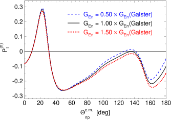
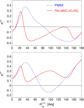
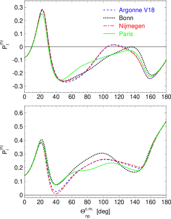
References
- (1) D. R. Yennie, M. M. Lévy, and D. G. Ravenhall, Rev. Mod. Phys. 29, 144 (1957); F. J. Ernst, R. G. Sachs, and K. C. Wali, Phys. Rev. 119, 1105 (1960); R. G. Sachs, Phys. Rev. 126, 2256 (1962); L. N. Hand, D. G. Miller, and R. Wilson, Rev. Mod. Phys. 35, 335 (1963).
- (2) S. Frullani and J. Mougey, Adv. Nucl. Phys. 14, 1 (1984).
- (3) D. Drechsel and M. M. Giannini, Rep. Prog. Phys. 52, 1083 (1989).
- (4) I. Sick, Prog. Part. Nucl. Phys. 47, 245 (2001).
- (5) A. W. Thomas and W. Weise, The Structure of the Nucleon (Wiley-VCH, Berlin, 2001).
- (6) H. Gao, Int. J. Mod. Phys. E 12, 1 (2003); H. Gao, Int. J. Mod. Phys. E 12, 567 (2003).
- (7) C. E. Hyde-Wright and K. de Jager, Annu. Rev. Nucl. Part. Sci. 54, 217 (2004).
- (8) A. Lung et al., Phys. Rev. Lett. 70, 718 (1993).
- (9) S. Platchkov et al., Nucl. Phys. A510, 740 (1990).
- (10) R. Madey and T. Eden, Fizika B (Zagreb) 8, 35 (1999); Jefferson Laboratory experiment 93-038, R. Madey and S. Kowalski, spokespersons.
- (11) R. Madey et al., Phys. Rev. Lett. 91, 122002 (2003).
- (12) B. Plaster, Ph.D. thesis, Massachusetts Institute of Technology (2003); S. Tajima, Ph.D. thesis, Duke University (2003); W. Tireman, Ph.D. thesis, Kent State University (2003); G. MacLachlan, Ph.D. thesis, Ohio University (2004); A. Aghalaryan, Ph.D. thesis, Yerevan Physics Institute (in preparation); E. Crouse, Ph.D. thesis, The College of William and Mary (in preparation).
- (13) A. I. Akhiezer, L. N. Rozentsveig, and I. M. Shmushkevich, Sov. Phys. JETP 6, 588 (1958).
- (14) N. Dombey, Rev. Mod. Phys. 41, 236 (1969).
- (15) A. I. Akhiezer and M. P. Rekalo, Sov. J. Part. Nucl. 4, 277 (1974).
- (16) R. G. Arnold, C. E. Carlson, and F. Gross, Phys. Rev. C 23, 363 (1981).
- (17) M. Ostrick et al., Phys. Rev. Lett. 83, 276 (1999).
- (18) H. Arenhövel, Phys. Lett. B 199, 13 (1987).
- (19) H. Arenhövel, W. Leidemann, and E. L. Tomusiak, Z. Phys. A 331, 123 (1988); H. Arenhövel, W. Leidemann, and E. L. Tomusiak, Z. Phys. A 334, 363 (1989).
- (20) M. P. Rekalo, G. I. Gakh, and A. P. Rekalo, J. Phys. G 15, 1223 (1989).
- (21) J. M. Laget, Phys. Lett. B 273, 367 (1991).
- (22) T. W. Donnelly and A. S. Raskin, Ann. Phys. 169, 247 (1986); A. S. Raskin and T. W. Donnelly, Ann. Phys. 191, 78 (1989).
- (23) C. Y. Cheung and R. M. Woloshyn, Phys. Lett. 127B, 147 (1983).
- (24) E. L. Tomusiak and H. Arenhövel, Phys. Lett. B 206, 187 (1988).
- (25) H. Arenhövel, W. Leidemann, and E. L. Tomusiak, Phys. Rev. C 46, 455 (1992); H. Arenhövel, W. Leidemann, and E. L. Tomusiak, Phys. Rev. C 52, 1232 (1995).
- (26) W. Leidemann, E. L. Tomusiak, and H. Arenhövel, Phys. Rev. C 43, 1022 (1991).
- (27) B. Blankleider and R. M. Woloshyn, Phys. Rev. C 29, 538 (1984).
- (28) C. Ciofi degli Atti, E. Pace, and G. Salmè, Phys. Rev. C 46, R1591 (1992).
- (29) R.-W. Schulze and P. U. Sauer, Phys. Rev. C 48, 38 (1993).
- (30) R. Schiavilla and I. Sick, Phys. Rev. C 64, 041002(R) (2001).
- (31) C. E. Jones-Woodward et al., Phys. Rev. C 44, R571 (1991).
- (32) A. K. Thompson et al., Phys. Rev. Lett. 68, 2901 (1992).
- (33) T. Eden et al., Phys. Rev. C 50, R1749 (1994).
- (34) P. Markowitz et al., Phys. Rev. C 48, R5 (1993).
- (35) H. Gao et al., Phys. Rev. C 50, R546 (1994); H. Gao, Nucl. Phys. A631, 170c (1998).
- (36) S. Galster et al., Nucl. Phys. B32, 221 (1971).
- (37) M. Meyerhoff et al., Phys. Lett. B 327, 201 (1994).
- (38) J. Becker et al., Eur. Phys. J. A 6, 329 (1999).
- (39) J. Golak et al., Phys. Rev. C 63, 034006 (2001).
- (40) C. Herberg et al., Eur. Phys. J. A 5, 131 (1999).
- (41) I. Passchier et al., Phys. Rev. Lett. 82, 4988 (1999).
- (42) D. Rohe et al., Phys. Rev. Lett. 83, 4257 (1999).
- (43) J. Bermuth et al., Phys. Lett. B 564, 199 (2003).
- (44) G. Kubon et al., Phys. Lett. B 524, 26 (2002).
- (45) J. Golak et al., Phys. Rev. C 65, 044002 (2002).
- (46) W. Xu et al., Phys. Rev. Lett. 85, 2900 (2000); W. Xu et al., Phys. Rev. C 67, 012201(R) (2003).
- (47) G. Höhler et al., Nucl. Phys. B114, 505 (1976).
- (48) H. Zhu et al., Phys. Rev. Lett. 87, 081801 (2001).
- (49) J. J. Kelly, Phys. Rev. C 66, 065203 (2002).
- (50) G. Warren et al., Phys. Rev. Lett. 92, 042301 (2004).
- (51) D. I. Glazier et al., Eur. Phys. J. A 24, 101 (2005).
- (52) J. Friedrich and Th. Walcher, Eur. Phys. J. A 17, 607 (2003).
- (53) C. W. Leemann, D. R. Douglas, and G. A. Krafft, Annu. Rev. Nucl. Part. Sci. 51, 413 (2001).
- (54) R. Madey, A. Lai, and T. Eden, A.I.P. Conf. Proc. 339, 47 (1995); I. Niculescu et al., IEEE Trans. Nucl. Sci. 45, 68 (1998).
- (55) M. Poelker et al., A.I.P. Conf. Proc. 570, 943 (2001).
- (56) M. Poelker and J. Hansknecht, Proceedings of the IEEE Particle Accelerator Conference (PAC 2001), 95 (2001).
- (57) C. Yan et al., Nucl. Instrum. Methods Phys. Res. A 365, 261 (1995).
- (58) M. Hauger et al., Nucl. Instrum. Methods Phys. Res. A 462, 382 (2001).
- (59) J. Alcorn et al., Nucl. Instrum. Methods Phys. Res. A 522, 294 (2004).
- (60) C. Yan et al., Nucl. Instrum. Methods Phys. Res. A 365, 46 (1995); R. Wojcik and C. Yan, Nucl. Instrum. Methods Phys. Res. A 484, 690 (2002).
- (61) O. K. Baker et al., Nucl. Instrum. Methods Phys. Res. A 367, 92 (1995).
- (62) L. Wolfenstein, Phys. Rev. 75, 1664 (1949); L. Wolfenstein, Phys. Rev. 85, 947 (1952).
- (63) J. Simkin and C. W. Trowbridge, Rutherford Laboratory Report 79-097 (unpublished).
-
(64)
S. Taylor, E93-038 technical reports (unpublished):
http://www.jlab.org/plaster/reports/charybdis1.ps; http://www.jlab.org/plaster/reports/charybdis2.ps; http://www.jlab.org/plaster/reports/charybdis3.ps. - (65) R. Madey et al., Nucl. Instrum. Methods Phys. Res. 214, 401 (1983).
- (66) J. W. Watson et al., Nucl. Instrum. Methods Phys. Res. A 272, 750 (1988); R. Madey et al., IEEE Trans. Nucl. Sci 36, 231 (1989). T. Eden et al., Nucl. Instrum. Methods Phys. Res. A 338, 432 (1994).
- (67) http://coda.jlab.org.
- (68) J. Arrington, Ph.D. thesis, California Institute of Technology (1998).
- (69) R. Madey et al., Nucl. Instrum. Methods Phys. Res. 151, 445 (1978).
- (70) R. A. Arndt, I. I. Strakovsky, and R. L. Workman, Int. J. Mod. Phys. A 18, 449 (2003).
- (71) G. G. Ohlsen and P. W. Keaton, Jr., Nucl. Instrum. Methods Phys. Res. 109, 41 (1973).
- (72) D. L. Prout et al., Phys. Rev. C 63, 014603 (2000).
- (73) J. Arrington, SIMC computer code, http://www.jlab.org/johna/SIMC_documents/simc.ps.
- (74) R. Machleidt, K. Holinde, and Ch. Elster, Phys. Rep. 149, 1 (1987).
- (75) R. W. Finlay et al., Phys. Rev. C 47, 237 (1993).
- (76) R. A. Cecil, B. D. Anderson, and R. Madey, Nucl. Instrum. Methods Phys. Res. 161, 439 (1979).
- (77) S. Kopecky et al., Phys. Rev. Lett. 74, 2427 (1995); S. Kopecky et al., Phys. Rev. C 56, 2229 (1997).
- (78) J. J. Kelly, Phys. Rev. C 70, 068202 (2004).
- (79) E. J. Brash, A. Kozlov, Sh. Li, and G. M. Huber, Phys. Rev. C 65, 051001(R).
- (80) A. Afanasev, I. Akushevich, and N. Merenkov, Phys. Rev. D 64, 113009 (2001).
- (81) G. G. Simon, C. Schmitt, F. Borkowski, and V. H. Walther, Nucl. Phys. A333, 381 (1980).
- (82) L. E. Price et al., Phys. Rev. D 4, 45 (1971).
- (83) M. K. Jones et al., Phys. Rev. Lett. 84, 1398 (2000); O. Gayou et al., Phys. Rev. C 64, 038202 (2001); V. Punjabi et al., Phys. Rev. C 71, 055202 (2005).
- (84) O. Gayou et al., Phys. Rev. Lett. 88, 092301 (2002).
- (85) T. Pospischil et al., Eur. Phys. J. A 12, 125 (2001).
- (86) B. D. Milbrath et al., Phys. Rev. Lett. 82, 2221 (1999).
- (87) H. Anklin et al., Phys. Lett. B 336, 313 (1994).
- (88) H. Anklin et al., Phys. Lett. B 428, 248 (1998).
- (89) F. Iachello, A. D. Jackson, and A. Lande, Phys. Lett. 43B, 191 (1973).
- (90) M. F. Gari and W. Krümpelmann, Z. Phys. A 322, 689 (1985).
- (91) M. F. Gari and W. Krümpelmann, Phys. Lett. B 274, 159 (1992).
- (92) R. Bijker and F. Iachello, Phys. Rev. C 69, 068201 (2004).
- (93) E. L. Lomon, Phys. Rev. C 64, 035204 (2001).
- (94) E. L. Lomon, Phys. Rev. C 66, 045501 (2002).
- (95) Jefferson Laboratory experiment 02-013, G. Cates, K. McCormick, B. Reitz, and B. Wojtsekhowski, spokespersons.
- (96) Jefferson Laboratory experiment 04-110, B. Anderson, J. Kelly, S. Kowalski, R. Madey, and A. Semenov, spokespersons.
- (97) D. H. Lu, A. W. Thomas, and A. G. Williams, Phys. Rev. C 57, 2628 (1998).
- (98) A. L. Licht and A. Pagnamenta, Phys. Rev. D 2, 1150 (1970).
- (99) D. H. Lu, K. Tsushima, A. W. Thomas, and A. G. Williams, Nucl. Phys. A634, 443 (1998).
- (100) D. Lu, K. Tsushima, A. W. Thomas, A. G. Williams, and K. Saito, Phys. Rev. C 60, 068201 (1999).
- (101) S. Dieterich et al., Phys. Lett. B 500, 47 (2001).
- (102) S. Strauch et al., Phys. Rev. Lett. 91, 052301 (2003).
- (103) G. A. Miller and M. R. Frank, Phys. Rev. C 65, 065205 (2002); G. A. Miller, Phys. Rev. C 66, 032201(R) (2002).
- (104) M. R. Frank, B. K. Jennings, and G. A. Miller, Phys. Rev. C 54, 920 (1996).
- (105) T. Fuchs, J. Gegelia, and S. Scherer, J. Phys. G 30, 1407 (2004).
- (106) M. R. Schindler, J. Gegelia, and S. Scherer, Nucl. Phys. B682, 367 (2004).
- (107) H.-W. Hammer, D. Drechsel, and U.-G. Meissner, Phys. Lett. B 586, 291 (2004).
- (108) M. R. Schindler, J. Gegelia, and S. Scherer, arXiv:nucl-th/0509005.
- (109) M. M. Kaskulov and P. Grabmayr, Phys. Rev. C 69, 028201 (2004); M. M. Kaskulov and P. Grabmayr, Eur. Phys. J. A 19, 157 (2004).
- (110) R. F. Wagenbrunn, S. Boffi, W. Klink, W. Plessas, and M. Radici, Phys. Lett. B 511, 33 (2001); S. Boffi, L. Ya. Glozman, W. Klink, W. Plessas, M. Radici, and R. F. Wagenbrunn, Eur. Phys. J. A 14, 17 (2002).
- (111) S. Simula, arXiv:nucl-th/0105024.
- (112) F. Cardarelli, E. Pace, G. Salmè, and S. Simula, Phys. Lett. B 357, 267 (1995).
- (113) M. De Sanctis, M. M. Giannini, E. Santopinto, and A. Vassallo, arXiv:nucl-th/0506033.
- (114) M. Göckeler et al., Phys. Rev. D 71, 034508 (2005).
- (115) J. D. Ashley, D. B. Leinweber, A. W. Thomas, and R. D. Young, Eur. Phys. J. A 19, 9 (2004).
- (116) H. H. Matevosyan, G. A. Miller, and A. W. Thomas, Phys. Rev. C 71, 055204 (2005).
- (117) H. Arenhövel, W. Leidemann, and E. L. Tomusiak, Eur. Phys. J. A 23, 147 (2005).
- (118) D. R. Giebink, Phys. Rev. C 32, 502 (1985).
- (119) H. Arenhövel, private communication (2001, 2002, 2003).
- (120) R. B. Wiringa, V. G. J. Stoks, and R. Schiavilla, Phys. Rev. C 51, 38 (1995).
- (121) M. M. Nagels, T. A. Rijken, and J. J. de Swart, Phys. Rev. D 17, 768 (1978).
- (122) M. Lacombe et al., Phys. Lett. 101B, 139 (1981).