The SAMPLE Experiment and Weak Nucleon Structure

Abstract

One of the key elements to understanding the structure of the nucleon is the role of its quark-antiquark sea in its ground state properties such as charge, mass, magnetism and spin. In the last decade, parity-violating electron scattering has emerged as an important tool in this area, because of its ability to isolate the contribution of strange quark-antiquark pairs to the nucleon’s charge and magnetism. The SAMPLE experiment at the MIT-Bates Laboratory, which has been focused on $\overline{s}s$ contributions to the proton’s magnetic moment, was the first of such experiments and its program has recently been completed. In this paper we give an overview of some of the experimental aspects of parity-violating electron scattering, briefly review the theoretical predictions for strange quark form factors, summarize the SAMPLE measurements, and place them in context with the program of experiments being carried out at other electron scattering facilities such as Jefferson Laboratory and the Mainz Microtron.

1 Introduction

Over the last decade, parity violating electron scattering has become a unique tool for probing the contribution of the nucleon’s sea of quark-antiquark pairs to its ground state electromagnetic structure. Improvements in experimental techniques, particularly in the development and delivery of intense and high quality polarized electron beams, have led to the ability to measure parity-violating asymmetries at the level of parts per million with relatively good precision. A few measurements from the first of these challenging experiments have now been completed, and several additional experiments are planned or underway. While theoretical advances have provided guidance as to the expected magnitude of sea quark contributions, robust predictions do not yet exist. In the next several years, a number of new measurements are expected to become available over a range of momentum transfers. These data should begin to constrain the various calculations and help identify both the magnitude of $s$-quark contributions and the mechanism by which they might be present. In addition, there is some promise that lattice QCD calculations, which have evolved significantly in the last several years, may be able to provide predictions to confront the data. In this paper we review the present state of experiment and theory with a specific emphasis on the SAMPLE experiment, which was carried out at the MIT-Bates Laboratory in the 1990’s and for which final analysis of the data has recently been completed [1, 2].

The outline of this paper is as follows: in this section we will give an overview of parity-violating electron scattering and its role in the determination of the quark structure of the nucleon’s electromagnetic form factors, particularly that of strange quark-antiquark pairs. We will also review some of the theoretical developments that have recently taken place. After an overview of some of the experimental issues, we provide an in-depth look at the SAMPLE experiment at the MIT-Bates Laboratory in Section 2. In Section 3 we will place the SAMPLE experiment in context with existing measurements from the HAPPEX program at Jefferson Laboratory and the PVA4 program at the MAMI facility in Mainz, Germany, as well as compare the various results with theoretical predictions. We will conclude with a discussion of the future program at Jefferson Laboratory (G⁰ and HAPPEX) and at Mainz, and make some brief remarks about future measurements that intend to use parity-violating electron scattering for precision tests of the Standard Model.

1.1 Weak Form Factors and the Role of Strange Quarks

The formalism of the electroweak interaction between electrons and quarks can be found in many textbooks and several recent reviews of parity violating electron scattering [3, 4, 5, 6]. Here we will largely follow the notation used in [6]. At low momentum transfer, the interaction of an electron with a nucleon is usually cast in these terms by defining a nucleon current for which the quark substructure is encapsulated in form factors that are the observables of the interaction. The invariant amplitudes associated with a single photon or $Z$-boson exchange are

$$M_{\gamma} = \frac{4\pi\alpha}{q^{2}}e_{l}l^{\mu}J_{\mu}^{EM}$$

$$M_{Z} = -\frac{G_{F}}{2\sqrt{2}}\left(g_{V}^{l}l^{\mu}+g_{A}^{l}l^{\mu 5}\right)\left(J_{\mu}^{NC}\right)\,$$ (1)

where $q$ is the four momentum transferred from the electron to the nucleon. Throughout this paper we will use the standard experimental notation for the four-vector momentum transfer squared, $Q^{2}=-q^{2}>0$. Note that the $Q^{2}$ dependence of the neutral weak propagator has been suppressed since, at momentum transfers that are small compared to the $Z$ and $W$ masses, the weak interaction is usually treated as a contact interaction with a strength determined by the Fermi decay constant $G_{F}=1.16639(1)\times 10^{-5}$ GeV^-2 [7]. The fermion electromagnetic and weak charges $e_{l}$, $g_{V}^{l}$, and $g_{A}^{l}$ are listed in Table 1.

Fermion	$e_{l}$	$g_{V}^{l}$	$g_{A}^{l}$
$\nu_{e}$, $\nu_{\mu}$, $\nu_{\tau}$	0	1	$-1$
$e$, $\mu$, $\tau$	$-1$	$-1+4\sin^{2}\theta_{W}$	1
$u$, $c$, $t$	$\frac{2}{3}$	$1-\frac{8}{3}\sin^{2}\theta_{W}$	$-1$
$d$, $s$, $b$	$-\frac{1}{3}$	$-1+\frac{4}{3}\sin^{2}\theta_{W}$	1

Table 1: Standard Model values for the elementary electromagnetic and weak charges of the fermions.

Because the electron is considered to be a pointlike particle with no structure, the leptonic currents $l^{\mu}$ and $l^{\mu 5}$ are simply $\overline{u}\gamma^{\mu}u$ and $\overline{u}\gamma^{\mu}\gamma_{5}u$, respectively. The nucleon currents, on the other hand, are expressed in terms of hadron form factors sandwiched between nucleon spinors,

$$J_{\mu}^{EM}\equiv\langle N|\hat{J}_{\mu}^{EM}|N\rangle = {\overline{U}}\left[\gamma_{\mu}F_{1}^{\gamma,N}(q^{2})+i\sigma_{\mu\nu}q^{\nu}\frac{F_{2}^{\gamma,N}}{2M}\right]U$$

$$J_{\mu}^{NC}\equiv\langle N|\hat{J}_{\mu}^{NC}|N\rangle = {\overline{U}}\left[\gamma_{\mu}F_{1}^{Z,N}(q^{2})+i\sigma_{\mu\nu}q^{\nu}\frac{F_{2}^{Z,N}}{2M}+\gamma_{\mu}\gamma_{5}G_{A}^{Z,N}+\frac{q_{\mu}}{M}\gamma_{5}G_{P}\right]U\,.$$ (2)

For completeness, we have included the pseudoscalar form factor $G_{P}$ in this expression, however we will otherwise neglect it since it does not contribute to parity-violating electron scattering. The form factors are the observables in elastic electron scattering from a nucleon target. $F_{1}$ for the proton(neutron) is normalized to 1(0) at zero momentum transfer, and $F_{2}$ to the anomalous part of the magnetic moments. At relatively low momentum transfer, the Dirac and Pauli form factors $F_{1}$ and $F_{2}$ are commonly expressed as the Sachs form factors $G_{E}$ and $G_{M}$,

$$G_{E}=F_{1}+\frac{Q^{2}}{4M^{2}}F_{2}\,,\;G_{M}=F_{1}+F_{2}\,,$$ (3)

resulting in the normalization of $G_{E}^{\gamma}$ to 1(0) for the proton (neutron), and of $G_{M}^{\gamma}$ to the appropriate magnetic moment. An equivalent definition can be applied to the vector weak form factors $F_{1,2}^{Z,N}$.

The form factors can be related to their quark substructure by expressing them as a sum over contributions from each quark flavor. Traditionally, the contributions from the heavy quarks ($c$,$t$, and $b$) are neglected so that the form factors are written as contributions from $u$, $d$, and $s$ quarks, where each contribution is weighted by the appropriate quark charge from Table 1. The proton’s Sachs electromagnetic and vector neutral weak form factors become

$$G_{E,M}^{\gamma} = \frac{2}{3}G_{E,M}^{u}-\frac{1}{3}\left(G_{E,M}^{d}+G_{E,M}^{s}\right)$$

$$G_{E,M}^{Z} = \left(1-\frac{8}{3}\sin^{2}\theta_{W}\right)G_{E,M}^{u}+\left(-1+\frac{4}{3}\sin^{2}\theta_{W}\right)\left(G_{E,M}^{d}+G_{E,M}^{s}\right)\,,$$ (4)

where, because the underlying vector current is the same for the photon and the $Z$-boson once the charges are factored out, these two expressions are just two different linear combinations of the same quark form factors.

If one next makes the assumption of charge symmetry in the nucleon, one can consider the neutron electromagnetic form factors as a third observable, and uniquely identify the three light quark contributions to the nucleon’s vector current. The assumption of charge symmetry implies that the wave function of the $u$ quarks in the proton are identical to the $d$ quarks in the neutron, or that $G_{E,M}^{u}$ and $G_{E,M}^{d}$ in the proton are simply interchanged in the neutron. With a small amount of algebra the proton’s weak form factor can then be rewritten in terms of observable proton and neutron $EM$ form factors along with a residual contribution from strange quarks, allowing direct access to the strange quark piece,

$$G_{E,M}^{Z}=\left(1-4\sin^{2}\theta_{W}\right)G_{E,M}^{\gamma,p}-G_{E,M}^{\gamma,n}-G_{E,M}^{s}\,.$$ (5)

The electroweak axial form factor of the nucleon can be similarly deconstructed to reveal the contribution of strange quarks to nucleon spin. In the lowest order limit of single $Z$-boson exchange, only the isovector and SU(3) singlet contributions survive, resulting in

$$G_{A}^{Z}(Q^{2})=-\tau_{3}G_{A}(Q^{2})+\Delta s$$ (6)

where $\tau_{3}=+1(-1)$ for $p(n)$, $G_{A}(0)=-(g_{A}/g_{V})=1.2670\pm 0.0035$ [7] as determined from $\beta$-decay experiments, and the quantity $\Delta s$ is the strange quark contribution to nucleon spin. As will be discussed later, the higher order corrections to $G_{A}^{Z}$ are expected to be significant. The $Q^{2}$-dependence of $G_{A}$ has been characterized by a dipole form factor, $1/(1+Q^{2}/M_{A}^{2})^{2}$, with the dipole mass $M_{A}$ experimentally determined from neutrino scattering and from pion electroproduction. The value of $M_{A}$ from electroproduction, which was measured to be 1.069$\pm$0.016 GeV [8], must be corrected for contributions from higher order processes in order to directly compare with results from neutrino scattering [9], leading to a corrected value of 1.014$\pm$0.016 GeV. The value of $M_{A}$ from neutrino scattering has also recently been reevaluated, by refitting the neutrino data using updated nucleon electromagnetic form factors [10]. This has shifted $M_{A}$ from the PDG world average of 1.026$\pm$0.02 GeV [7] to a new value of 1.001$\pm$0.020 GeV, now in good agreement with the electroproduction data.

The fact that one can uniquely extract information about strange quark effects in the nucleon from elastic neutral-current processes was pointed out by Kaplan and Manohar in 1988 [11]. Soon after, McKeown [12] and Beck [13] showed how $G_{E,M}^{Z}$ could be measured using parity-violating electron scattering, which led to the program of experiments at MIT-Bates, Jefferson Laboratory, and the Mainz Microtron that are the focus of this review.

The parity-violating component of the amplitude in equation 1.1 arises from the cross terms of the axial and vector currents,

$$M_{PV}=-\frac{G_{F}}{2\sqrt{2}}\left(g_{A}^{l}l^{\mu 5}J^{NC}_{\mu}+g_{V}^{l}l^{\mu}J^{NC}_{\mu 5}\right)\,$$ (7)

where the nucleon current has now been separated into its vector and axial vector components. In order to observe this PV amplitude experimentally, one typically uses a longitudinally polarized beam and an unpolarized target and looks at the relative difference in cross section for the scattering as one flips the polarization of the incident beam along or against its momentum direction, i.e. between its right-handed and left-handed helicity states. This difference is directly proportional to the interference between $M_{\gamma}$ and $M_{PV}$. For elastic scattering from a spin-1/2 target such as a nucleon, the asymmetry can be written as

$$A_{PV}=\frac{d\sigma_{R}-d\sigma_{L}}{d\sigma_{R}+d\sigma_{L}}\,=-\frac{G_{F}Q^{2}}{4\pi\alpha\sqrt{2}}\frac{A_{E}+A_{M}+A_{A}}{\left[\varepsilon\left(G_{M}^{\gamma}\right)^{2}+\tau\left(G_{M}^{\gamma}\right)^{2}\right]}$$ (8)

where

$$A_{E} = \varepsilon G_{E}^{Z}(Q^{2})G_{E}^{\gamma}(Q^{2})$$

$$A_{M} = \tau G_{M}^{Z}(Q^{2})G_{M}^{\gamma}(Q^{2})$$

$$A_{A} = -\left(1-4\sin^{2}\theta_{W}\right)\sqrt{\tau\left(1+\tau\right)\left(1-\varepsilon^{2}\right)}G_{A}^{e}(Q^{2})G_{M}^{\gamma}(Q^{2})\,,$$ (9)

and

$$\tau=\frac{Q^{2}}{4M_{N}^{2}}\;,\mathrm{and}\;\varepsilon=\frac{1}{1+2\left(1+\tau\right)\tan^{2}\frac{\theta}{2}}\,.$$ (10)

The $\gamma$-$Z$ interference is explicitly seen in these expressions. Depending on the kinematics, one can tune an experiment to be sensitive to the electric, magnetic, or axial form factors. Forward angle experiments are typically sensitive to a combination of $A_{E}$ and $A_{M}$, while backward angle experiments determine a combination of $A_{M}$ and $A_{A}$. Quasielastic scattering from an isospin 0 target such as the deuteron can be used to enhance $A_{A}$; this is discussed in more detail below.

Charge Symmetry Violation

Isospin violation, or less restrictively charge symmetry breaking, invalidates the assumption that the $u$-quark wave function in the proton is identical to the $d$-quark wave function in the neutron and would lead to an additional term in $G_{E,M}^{Z}$ that would be indistinguishable from $G_{E,M}^{s}$. This violation arises from $u$ and $d$ quark mass differences and from electromagnetic effects. Dmitrasinovic and Pollock [14] and Miller [15] both calculated a charge symmetry breaking term within the context of a non-relativistic constituent quark model. In such a model, the size of the effect is driven by the ratio of the mass difference to the constituent quark mass, about 1/70, and results in fractional contributions to the isoscalar electric and magnetic form factors on the order of 0.1%. These models would thus predict that the precision of the strange quark measurements would have to be better than this level before charge symmetry breaking adds significant uncertainty to their determination. Similar conclusions were reached by Lewis and Mobed [16], who used a two-flavor heavy baryon chiral perturbation theory (HB$\chi$PT) to investigate the effects of isospin breaking.

Electroweak Radiative Corrections

Higher order diagrams, such as those depicted in Figure 1, have been treated by several authors. The corrections to the vector weak form factors tend to be dominated by terms involving a single quark and can be directly computed within the context of the Standard Model. They have been calculated at low energy (see references in [7]), and at the low values of momentum transfer relevant to the experiments described here, the dependence on $Q^{2}$ is relatively weak. These contributions have the same $(1-4\sin^{2}\theta_{W})$ multiplier as the tree-level amplitudes and thus are typically quite small. The one-quark axial corrections can also be computed in a model-independent fashion with relatively small uncertainty but they are substantial relative to the tree-level contribution. Of more concern in the axial radiative corrections are the potentially large contributions from diagrams involving two or more quarks. One class of such diagrams, referred to as “anapole” terms, involve an electromagnetic interaction with the scattered electron but weak interactions within the target. The calculations of weak radiative corrections most relevant to this paper are those of Musolf and Holstein [17] and of Zhu et al. [18]. In [17], the many-quark corrections are modeled as effective parity-violating hadronic couplings within the nucleon with the photon coupling to the nucleon via a meson loop. The dominant source of uncertainty results from the uncertainties in the hadronic couplings as determined by Desplanques, Donoghue and Holstein [19]. Zhu et al. [18] carried out a similar analysis, but recast the hadronic couplings in a heavy baryon chiral perturbation theory framework. All contributions through ${\cal O}(1/\Lambda_{\chi})$ were included, where $\Lambda_{\chi}=4\pi F_{\pi}$ is the scale of chiral-symmetry breaking. Potential contributions from additional mesons, as well as couplings involving kaons, were also included. The terms involving kaon loops were generally found to be small compared with those involving pions. As in the previous analysis, it was found that the one-quark axial corrections dominate the magnitude of the correction, whereas the multiquark terms dominate its uncertainty.

Incorporating the higher order terms as weak radiative corrections leads to the following modification of equation 5:

$$G_{E,M}^{Z}=\left(1-4\sin^{2}\theta_{W}\right)\left(1+R_{V}^{p}\right)G_{E,M}^{\gamma,p}-\left(1+R_{V}^{n}\right)G_{E,M}^{\gamma,n}-G_{E,M}^{s}\,$$ (11)

where the corrections to $G_{E,M}^{s}$ are left as implicit. The axial form factor is also modified, and the notation changed to $G_{A}^{e}$, in order to distinguish the form factor as seen by electron-scattering from that seen by neutrino scattering where the higher order diagrams involving a photon are absent, giving

$$G_{A}^{e}(Q^{2})=-\tau_{3}(1+R_{A}^{T=1})G_{A}+\sqrt{3}R_{A}^{T=0}G_{A}^{8}+\Delta s\,.$$ (12)

There is now explicitly a term proportional to an SU(3) isoscalar octet form factor $G_{A}^{8}$, which at tree-level is zero. The magnitude of this form factor is estimated (it has not been directly measured) using the ratio of axial vector to vector couplings in hyperon beta decay, which, assuming SU(3) flavor symmetry, can be related to the octet axial charge $a_{8}$ and to $F$ and $D$ coefficients [7].

$$G_{A}^{8}(0)=\frac{(3F-D)}{2\sqrt{3}}=\frac{1}{2}a_{8}=\frac{\sqrt{3}}{2}(-0.25\pm 0.05)=0.217\pm 0.043\,.$$ (13)

The $Q^{2}$ dependence is also not measured, but can be estimated using the same dipole mass behavior as for the isovector axial form factor. This results in a net isoscalar octet correction that we define as $R_{A}^{0}=\sqrt{3}R_{A}^{T=0}G_{A}^{8}(Q^{2})$, which for $Q^{2}=0.1$ (GeV/c)² is $0.02\pm 0.04$. Table 2 contains the values of the vector and axial vector weak radiative corrections used in computing the parity-violating asymmetry relevant to the SAMPLE experiment.

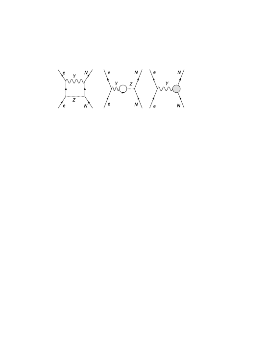
Figure 1: Higher order corrections, such as $\gamma$-$Z$ box diagrams (a), $\gamma$-$Z$ mixing corrections (b), and vertex corrections (c), that contribute to the neutral current scattering amplitude. The third diagram can involve a $Z$ exchange between two quarks in the nucleon. Both (b) and (c) are classified as “anapole” corrections.

correction	$T=0$	$T=1$
$R_{V}$	$-0.0113$	$-0.017\pm 0.002$
$R_{A}$	$0.06\pm 0.14$	$-0.23\pm 0.24$

Table 2: Values of electroweak radiative corrections to parity-violating electron scattering, as described in the text, computed in the $\overline{MS}$ scheme. The vector corrections are taken from [6], and the axial corrections are taken from [18] after the 1-quark corrections are converted to their $\overline{MS}$ values. Note that the nucleon vector corrections $R_{V}^{p}=[(1-2\sin^{2}\theta_{W})R_{V}^{(T=1)}-2\sin^{2}\theta_{W}R_{V}^{(T=0)}]/(1-4\sin^{2}\theta_{W})=-0.054\pm 0.033$ and $R_{V}^{n}=(1-2\sin^{2}\theta_{W})R_{V}^{(T=1)}+2\sin^{2}\theta_{W}R_{V}^{(T=0)}=-0.0143\pm 0.0004$ are used in the text.

Sensitivity to Nucleon Electromagnetic Form Factors

An important consideration in extracting the strange vector form factors is the quality of information known about the nucleon’s electromagnetic structure. An interesting consequence of the isospin structure of the neutral weak interaction is that, as can be observed in equation 5, determination of the strange quark form factors of the proton requires good knowledge of the neutron’s electromagnetic properties.

Precise determination of $G_{E}^{\gamma}$ and $G_{M}^{\gamma}$ for both the proton and neutron has been a topic of intense activity at all of the electron scattering laboratories over the last decade and significant progress has been made in recent years. The majority of the information on the proton charge and magnetic form factors comes from unpolarized electron scattering experiments. In the one-photon exchange approximation, the $e$-$p$ elastic scattering cross section in the laboratory frame can be written as

$$\frac{d\sigma}{d\Omega}=\left(\frac{\alpha^{2}\cos^{2}\frac{\theta}{2}}{4E^{2}\sin^{4}\frac{\theta}{2}}\right)\frac{E^{\prime}}{E}\frac{1}{\varepsilon\left(1+\tau\right)}\left[\varepsilon\left(G_{E}^{\gamma}\right)^{2}+\tau\left(G_{M}^{\gamma}\right)^{2}\right]\,$$ (14)

and through measurements at various scattering angles one can separate the electric and magnetic pieces [20]. Very recently, this “Rosenbluth” technique has come under some degree of scrutiny because of new results from polarization experiments that are in conflict with the results from the unpolarized data at momentum transfers above 1 (GeV/c)². While we will not attempt a detailed review of this topic, some brief remarks are in order.

With a polarized beam and either a polarized target or detection of the polarization of the recoiling nucleon it is possible to determine directly either the ratio of $G_{E}^{\gamma}/G_{M}^{\gamma}$, or the product $G_{E}^{\gamma}G_{M}^{\gamma}$ in a single measurement. These techniques do not require an absolute determination of the experimental cross section and are thus less susceptible to experimental systematic uncertainties related to knowledge of detector acceptance, absolute beam flux, or detector efficiencies. They are also less sensitive to corrections beyond the one-photon exchange approximation. With a longitudinally polarized beam and detection of the recoil polarization, the ratio of polarization components perpendicular and parallel to the nucleon’s momentum determines the ratio [21, 22, 23, 24]

$$\frac{G_{E}^{\gamma}}{G_{M}^{\gamma}}=-\frac{P_{T}}{P_{L}}\frac{E_{e}+E_{e}^{\prime}}{2M_{N}}\tan\frac{\theta_{e}}{2}\,,$$ (15)

where $(E_{e},E_{e}^{\prime},\theta_{e})$ are the incident and scattered electron energy and electron laboratory scattering angle, respectively.

Recently, data have been taken at Jefferson Laboratory using the recoil polarization technique for $e$-$p$ scattering [25, 26, 27] in which a monotonic decrease of $\frac{G_{E}^{\gamma}}{G_{M}^{\gamma}}$ with increasing $Q^{2}$ was found. This is in contrast to a global analysis of the world’s set of Rosenbluth data that seemed to indicate a more constant ratio [28]. New cross section data from Jefferson Laboratory are in good agreement with the older cross section data [29]. Radiative corrections coming from two-photon exchange introduce an additional $\varepsilon$-dependence to the cross section that distort the relative contributions of $G_{E}^{p}$ and $G_{M}^{p}$, complicating the Rosenbluth extraction at high momentum transfer where the $\varepsilon$-dependent term is typically only a small fraction of the cross section. Preliminary calculations that do not include intermediate states of the nucleon indicate that two-photon exchange can account for at least half of the discrepancy between the two data sets [30, 31], as well as for differences between electron-proton and positron-proton scattering [32]. New experiments are underway that will provide additional data on the proton form factors at high momentum transfer [33, 34] and new measurements are being proposed to explicitly measure two-photon exchange processes [35]. At the time of this writing, the discrepancy between the results from the unpolarized cross section data and the polarization measurements has yet to be completely resolved. At the momentum transfers of interest to the discussion here (below 1 (GeV/c)²), the data from the two methods agree within experimental uncertainties and both of the proton’s electromagnetic form factors are taken to be known to 2% [32]. Polarized targets have not been used in the past to determine proton EM form factors, but an experiment is planned at the MIT-Bates Laboratory in the near future [37] using this technique.

It should also be noted that experiments with an unpolarized target and transversely polarized beam are directly sensitive to the imaginary part of the two-photon amplitudes. Experimentally one measured an azimuthal dependence to the yield asymmetry. Such measurements can typically be performed to ppm-level precision in a few days in a parity-violation experiment setup. While these imaginary components do not influence the radiative corrections that enter the cross section measurements, their determination can provide additional constraints on the theory. As will be discussed below, data presently exist from the SAMPLE and PVA4 experiments and are expected from the G0 experiment.

While the neutron’s electromagnetic structure is not yet known to this degree of precision, considerable progress has been made in recent years. In fact, it is the neutron form factors to which the parity violation experiments that seek to extract strange quark information are more sensitive because, to lowest order, the neutron’s vector neutral weak charge is large relative to that of the proton. The majority of the new measurements of the neutron’s electric and magnetic form factors have used polarization techniques and, by necessity, light nuclear targets, causing an additional level of complexity in extracting the form factors.

With a polarized beam and a polarized target, the differential cross section for elastic scattering has an additional spin-dependent term $\Delta$,

$$\frac{d\sigma}{d\Omega}=\Sigma+h\Delta$$ (16)

that depends on the electron beam helicity, $h$=$\pm$1. The unpolarized differential cross section $\Sigma$ was defined in eq. (14). By reversing the electron beam helicity and measuring the asymmetry in the count rate for a given target polarization, the spin-dependent term can be isolated, through the spin-dependent yield asymmetry

$$A = \frac{d\sigma^{+}-d\sigma^{-}}{d\sigma^{+}+d\sigma^{-}}$$ (17)

$$= \frac{\Delta}{\Sigma}=-\frac{2\tau v_{T^{\prime}}\cos\theta^{*}\left(G_{M}^{\gamma}\right)^{2}+2\sqrt{2\tau\left(1+\tau\right)}v_{TL^{\prime}}\sin\theta^{*}\cos\phi^{*}G_{M}^{\gamma}G_{E}^{\gamma}}{\left(1+\tau\right)v_{L}\left(G_{E}^{\gamma}\right)^{2}+2\tau v_{T}\left(G_{M}^{\gamma}\right)^{2}}\,,$$

where $(\theta^{*},\phi^{*})$ define the direction of the target polarization with respect to the three-momentum transfer vector ${\bf q}$ and the $e$-$p$ scattering plane, and $v_{i}$ are kinematic factors. Polarized deuterium and ³He targets have been used to extract neutron form factors, where the use of polarization observables has provided a significant reduction in the nuclear model dependence. A recent review of the various experimental techniques can be found in [36]. Here we simply highlight the particularly notable features of the recent progress relevant to the determination of strange quark form factors.

A series of experiments was carried out at Jefferson Laboratory with a polarized ³He target to determine $G_{M}^{n}$ up to a momentum transfer of 1 (GeV/c)² [38, 39]. In these measurements, it was found that below $Q^{2}\sim 0.3$ (GeV/c)² final state interaction effects modify the asymmetry significantly, requiring the use of a state-of-the-art three-nucleon wave function to relate the asymmetry to the neutron form factor. Above 0.3 (GeV/c)², final state interactions are less important but relativistic corrections become significant, so a PWIA calculation that includes relativistic corrections was used to extract $G_{M}^{n}$. The data are shown in Figure 2 as the solid circles. The $\vec{{}^{3}\mathrm{He}}(\vec{e},e^{\prime})$ asymmetry measurements can be compared to another recent determination of $G_{M}^{n}$ using the ratio of unpolarized cross sections $d(e,e^{\prime}n)/(e,e^{\prime}p)$ [40], shown as the solid diamonds in Figure 2. Nuclear structure effects cancel to a large extent in the ratio, and the dominant uncertainty in the measurement comes from absolute knowledge of the neutron detection efficiency. This has been a source of discrepancy between past measurements [41, 42]. In [40] the neutron detection efficiency was measured using tagged and monoenergetic neutron beams with a claimed accuracy of 1%, resulting in an uncertainty in $G_{M}^{n}$ of less than 2%. The agreement between these two most recent determinations of $G_{M}^{n}$, using quite different experimental techniques with very different theoretical uncertainties, is remarkable. A new experiment using the cross section ratio technique, has recently been completed at JLab, which will push the measurements to higher momentum transfer [43]. So while precise information at high momentum transer is still pending, the low-momentum transfer data have now reached a level of precision comparable to our knowledge of $G_{M}^{p}$.

There has also been much recent progress on the neutron’s electric form factor. Initial polarization measurements demonstrated the feasibility of extracting $G_{E}^{n}$ in a somewhat model-dependent way, but were limited by statistical precision. Schiavilla and Sick [44] showed recently that one can reduce the model uncertainties in extracting $G_{E}^{n}$ from elastic $e$-$d$ scattering data by using only the deuteron’s quadrupole form factor, which has been experimentally determined from the deuteron’s tensor polarization [45] and is much less sensitive to uncertain short-range two-body currents in the deuteron. Two recent JLab experiments, one using a polarized target [47] and the other using recoil polarimetry [46], now provide the first double polarization measurements at momentum transfers above 1 (GeV/c)². The measurements are in good agreement with each other, and, combined with recent results from Mainz at lower momentum transfer using ${}^{3}\vec{\mathrm{He}}$ and $\vec{d}$ targets [48, 49], have greatly improved our knowledge of $G_{E}^{n}$. The BLAST collaboration at MIT-Bates [37] will take data using both ${}^{3}\vec{\mathrm{He}}$ and $\vec{d}$ targets at low momentum transfer over the next year, providing additional systematic checks of the nuclear structure contributions. It should be noted that uncertainties in $G_{E}^{n}$ at the 10% level will not significantly impact the extraction of the strange quark form factors with the proposed level of precision of the near term parity violation experiments.

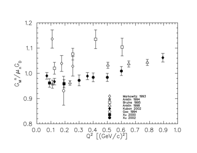
Figure 2: Recent measurements of the neutron’s magnetic form factor. Figure taken from [36]. The two most recent data sets are from [39] (solid circles) in which the asymmetry in $\vec{{}^{3}\mathrm{He}}(\vec{e},e^{\prime})$ was measured, and [40](solid diamonds) using the ratio of unpolarized cross sections $d(e,e^{\prime}n)/(e,e^{\prime}p)$.

1.2 Models of the Strange Vector Form Factors

Over the last decade a number of different models have been used as a context in which to estimate the magnitude of the strange quark vector form factors. A recent theoretical review of the origins of many of the models can be found in [4]: here we will simply give a qualitative picture and review some of the predictions. The nucleon has no net strangeness, so $G_{E}^{s}(0)$=0, but neither the sign nor the magnitude of $G_{M}^{s}(0)$, referred to in the literature as $\mu_{s}$, is yet known. It has become conventional to estimate the leading $Q^{2}$-dependence of $G_{M}^{s}$ and $G_{E}^{s}$, which are defined by a mean-square radius derived from the slopes at $Q^{2}=0$. We use the following definitions, used by Jaffe [50] and Musolf et al. [6]

$$r_{s}^{2} \equiv -6\frac{dF_{1}^{s}}{dQ^{2}}|_{Q^{2}=0}\,,$$

$$\mu_{s} = G_{M}^{s}(0)=F_{2}^{s}(0)$$

$$\rho_{s} \equiv \frac{dG_{E}^{s}}{d\tau}|_{Q^{2}=0}\,=-\frac{2}{3}M_{N}^{2}r_{s}^{2}-\mu_{s}\,.$$ (18)

“Poles” and Dispersion Relations

One of the earliest estimates of the magnitude of strange quark vector form factors came from Jaffe [50], who used a vector meson dominance (VMD) model and a dispersion analysis comparable to that used by Höhler [51] for the electromagnetic form factors. In the VMD framework, the $\sim\frac{1}{Q^{4}}$ “dipole” behavior of the nucleon form factors, ultimately arising from the quark-antiquark sea, is generated by intermediate state vector meson resonances such as the $\phi$ and $\omega$ and a higher mass meson that incorporates all additional unknown contributions. Höhler had noted that, in such a 3-pole fit to the form factors, a strong coupling to a meson with a mass close to the predominantly $s\overline{s}$ $\phi$ meson was required to get the dipole behavior. Using Höhler’s fit to the isoscalar form factors, the mixing of the physical $\omega$, $\phi$ from their pure $q\overline{q}$ states ($(u\overline{u}+d\overline{d})/\sqrt{2}$, and $\overline{s}s$, respectively) as determined by radiative $\phi$ decay, and assumptions about the asymptotic behavior of the form factors, the behavior of $F_{1}^{s}$ and $F_{2}^{s}$ at low momentum was deduced. The result was a value of $\mu_{s}\sim-0.3$ and $r_{s}^{2}\sim 0.15$ fm².

This analysis has been refined by several authors in various ways. Mergell, Meissner, and Drechsel [53] updated Höhler’s analysis including newer, more precise, form factor data and Hammer et al. [54] used the updated fit to revisit Jaffe’s analysis. They found $\mu_{s}$=$-0.24\pm 0.03$, and $r_{s}^{2}=(0.21\pm 0.03)$ fm². Forkel [52] also refit the data, finding similar results. He also revisited the asymptotic behavior used by Jaffe, requiring a better match to that predicted by quark counting rules at large momentum transfer. To change the asymptotic behavior he introduced additional poles, and thus additional fit parameters, but generally found this reduced both $r_{s}^{2}$ and $\mu_{s}$ by about a factor of 2.

Finally, in a series of papers, Hammer, Ramsey-Musolf, and collaborators [55, 56, 57, 58] took the dispersion relation analysis beyond the context of simple vector meson dominance and also studied possible continuum contributions, particularly that of $K\overline{K}$. They found that in a combined fit to the isoscalar (nonstrange) form factors most of the contribution to $F_{2}^{(I=0)}$ from the $\phi$-meson is taken up by the $K\overline{K}$ continuum. In the case of $F_{1}^{(I=0)}$, some strength from the $\phi$ remains, although good fits are also obtained if the $\phi$ strength is replaced with a $\rho-\pi$ continuum strength, leaving the role of the $\phi$-meson in the structure of $F_{1}$ more ambiguous. When they use the results of their fit to the EM form factors to extract the low-$Q^{2}$ behavior of the strange form factors, they get a comparable value for $\mu_{s}$, $-0.28$, as had been obtained in [50] and [54], but a significantly larger value for the electric strangeness radius $r_{s}^{2}$ =0.42 fm².

Kaon Loops

Another approach to estimating strange quark effects has been the “kaon loop” picture, where the origin of the spatial separation of $\overline{s}$ and $s$ comes from a $\Lambda$-$K$ component to the proton’s wave function. Typically these models predict a negative value for $r_{s}^{2}$, consistent with the picture of a $\Lambda$ core surrounded by a kaon cloud. Riska and collaborators [59] have also pointed out that this simple picture combined with helicity flip arguments would lead to a negative value of $\mu_{s}$.

A kaon cloud contribution within the context of a constituent quark model was considered by Koepf, Henley and Pollock [60]. They considered only contributions from the lightest kaons, and found that the use of pointlike quarks results in significant $s$-quark contributions but also in poor agreement with the nucleon’s measured electromagnetic properties. When they instead used a nucleon model with some spatial extent, such as a cloudy bag model, the result was very little contribution from strange quarks, an order of magnitude smaller than the estimate from the vector meson dominance models. However, their results are very sensitive to the choice of bag radius. Musolf and Burkardt [61] also looked predominantly at the contribution from ground state kaons but used hadron scattering data to constrain the form factors used at the meson-nucleon vertices. They also included seagull graphs required for gauge invariance. Adding these terms resulted in a value of $\mu_{s}$ again close to that of the vector meson dominance approach with little change to $r_{s}^{2}$. However, Geiger and Isgur showed that summing over a complete set of strange meson-baryon intermediate states results in cancellations that again reduce $\mu_{s}$ to a very small (and in their case positive) value [62].

Chiral Perturbation Theory

Recent efforts have been made to use chiral perturbation theory ($\chi$PT) to compute the leading $Q^{2}$ behavior of $G_{E}^{s}$ and $G_{M}^{s}$. At low energies, $\chi$PT has been enormously successful in describing a wide variety of observables and several authors have pursued the heavy-baryon version of $\chi$PT (HB$\chi$PT) to study nucleon form factors. In [63] Hemmert and collaborators showed that to one-loop order (or ${\cal O}(p^{3})$ where $p$ is the chiral expansion parameter), the $Q^{2}$ dependence of $G_{M}^{s}$ is free of unknown parameters, while $\mu_{s}$ requires knowledge of two unknown counterterms. Ramsey-Musolf and Ito [64] pointed out that higher order terms that could not be constrained by experiment would likely be as important in flavor singlet operators such as $\overline{s}\gamma_{\mu}s$. Nonetheless, Hemmert and collaborators combined their calculated $Q^{2}$-dependence for $G_{M}^{s}$ with the earliest results from SAMPLE [65] and HAPPEX [66] to predict the behavior of $G_{M}^{s}$ and $G_{E}^{s}$ over a broad range. They found that the two form factors must have opposite sign and result in $\rho_{s}=-0.8\pm 1.4$. The large uncertainty is driven primarily by extrapolation of the HAPPEX data back to $Q^{2}=0$. Recently, Hammer et al. [67] computed the $Q^{2}$-dependence of $G_{M}^{s}$ to next order in $\chi$PT and found the ${\cal O}(p^{4})$ to largely cancel the the ${\cal O}(p^{3})$ terms, leaving the leading behavior of $G_{M}^{s}$ to be determined by additional unknown constants such that even the sign of $\frac{dG_{M}^{s}}{dQ^{2}}$ is not known. Since experiments cannot directly measure $G_{M}^{s}(0)$, some form of extrapolation will be required to compare directly to calculations at this static limit. An experimental study of the $Q^{2}$ behavior of $G_{M}^{s}(Q^{2})$ is thus required. The authors of Ref. [67] formulate the extrapolation problem by writing $\mu_{s}$ as

$$\mu_{s}=G_{M}^{s}(Q^{2})-0.13b_{s}^{r}$$ (19)

where $b_{s}^{r}$ is the relevant unknown constant, giving a reasonable range from dimensional arguments of $|b_{s}^{r}|\leq 1$.

Lattice QCD

Ultimately, lattice QCD techniques will lead to the most rigorous theoretical prediction for the nucleon’s strange form factors. At present such calculations remain tremendously challenging because strange quark effects must inherently originate from disconnected insertions where the $\overline{s}s$ loops originate from the QCD vacuum. At present such a calculation remains prohibitively time consuming. The calculations to date are in quenched QCD and computed with a large pion mass so some form of extrapolation to a more physically meaningful situation is required. Dong and collaborators [68] carried out a lattice simulation with a relatively small number of gauge configurations, finding $\mu_{s}=-0.36\pm 0.20$ and a positive slope for $G_{E}^{s}$ at low momentum transfer. Lewis et al. [69] carried out a similar calculation but with a significantly larger number of gauge configurations and use of a chiral extrapolation to small pion masses, and found both form factors to be small over a range of momentum transfer. Their results were found to be consistent with the existing data and with a lattice-inspired calculation of Leinweber et al. [70].

A variety of other calculations of strange quark form factors have been carried out with different nucleon models; we will not attempt to describe them all here. These include chiral quark [59, 71, 72] and soliton-based [73, 74, 75] models, in which baryons are treated as a bound state of constituent quarks surrounded by a meson cloud, as well as Skyrme-type [76, 77] models. These models can eventually provide some guidance as to the origins of potential strange quark effects when the number and quality of the data points are sufficient to constrain them.

1.3 Weak Axial Form Factor and Quasielastic scattering from Deuterium

As described in Section 1.1, reliable extraction of the strange quark form factors from the parity-violating asymmetry also requires a determination of the proton’s effective axial form factor $G_{A}^{e}$, which is modified by electroweak radiative corrections that cannot yet be computed with high precision. The parity-violating asymmetry in quasielastic scattering is relatively insensitive to the strange quark form factors but is predominantly sensitive to $G_{A}^{e}$ and can thus provide experimental confirmation of the computed radiative corrections.

In the simplest, “static”, approximation where the two nucleons in the deuteron are treated as stationary, noninteracting particles, the parity-violating asymmetry in quasielastic $d(e,e^{\prime})$ is

$$A_{d}=\frac{\sigma_{p}A_{p}+\sigma_{n}A_{n}}{\sigma_{p}+\sigma_{n}}\,,$$ (20)

where $A_{p}$ is defined by equation 8, and $A_{n}$, the PV asymmetry for scattering from the neutron, is written by exchanging the neutron and proton indices in the form factors. At backward scattering angles where the asymmetry is predominantly sensitive to the magnetic and the axial vector contributions to $A$, it can be shown that the (isoscalar) strange quark contributions are multiplied by the isoscalar combination $G_{M}^{p}+G_{M}^{n}$ and are thus suppressed, whereas the non-strange (predominantly isovector) axial vector piece contains $G_{M}^{p}-G_{M}^{n}$ and is thus not suppressed. As a result, $A_{d}$ can be used as a control measurement for $G_{A}^{e}$ and its uncertain radiative corrections.

More generally, with moving and interacting nucleons, the asymmetry is dependent on both the momentum and energy transfer and is modified by NN interaction effects. The terms containing the nucleon form factors can instead be written as a ratio of response functions

$$A_{d}=\frac{G_{F}Q^{2}}{4\pi\alpha\sqrt{2}}\,\frac{W^{PV}}{W^{EM}}$$ (21)

where

$$W^{EM} = v_{L}R^{L}(q,\omega)+v_{T}R^{T}(q,\omega)$$

$$W^{PV} = v_{L}R_{AV}^{L}(q,\omega)+v_{T}R_{AV}^{T}(q,\omega)+v_{T^{\prime}}R_{VA}^{T^{\prime}}(q,\omega)$$ (22)

and the electron kinematic factors $v_{T}$, $v_{L}$ and $v_{T^{\prime}}$ are

$$v_{L}=\left[\frac{Q^{2}}{q^{2}}\right]^{2}\,,\>v_{T}=\frac{1}{2}\left|\frac{Q^{2}}{q^{2}}\right|+\tan^{2}\frac{\theta}{2}\,,\>{\mathrm{and}}\>v_{T^{\prime}}=\tan\frac{\theta}{2}\left[\left|\frac{Q^{2}}{q^{2}}\right|+\tan^{2}\frac{\theta}{2}\right]^{1/2}\,.$$ (23)

The response functions capture both the single nucleon currents and now also the corresponding two-nucleon currents. Studies of the effect of the NN interaction on the extraction of these single-nucleon quantities have been carried out by several authors, generally all leading to the conclusion that they tend to be small, although this conclusion depends somewhat on the details of the particular measurement. In [78], Hadjimichael, Poulis, and Donnelly looked at the sensitivity of the asymmetry to the choice of NN interaction, for example. They used several models and surveyed a range of kinematics, finding that at backward angles and moderate momentum transfers the PV asymmetry varies little with choice of model, whereas at either low momentum transfer or forward scattering angles bigger variations between models were found. The best sensitivity to the nucleon’s axial form factor is at backward angles, and near the kinematics the first SAMPLE experiment the NN model dependence appears to be at most a few percent. More recently, Diaconescu et al. [79] computed the effect of the parity-conserving components of two-body contributions on the parity-violating $e$-$d$ asymmetry using the Argonne V18 potential at the specific kinematics of the SAMPLE experiment, finding that these two-nucleon currents modify the asymmetry by up to 3% in the tails of the quasielastic distribution and closer to 0.5% near the quasielastic peak. Parity-violating two-nucleon contributions to the hadronic axial response function $R_{VA}^{T^{\prime}}$ were computed in [82], and recently again in [80, 81]. An example of the magnitude of the parity-violating NN contribution (labeled “DDH”) relative to the main one-body $\gamma$-$Z$ interference contribution, taken from [81], is shown in Figure 3. At the kinematics of interest here, these effects are about two orders of magnitude below the $\gamma$-$Z$ interference contribution, and are thus negligible. This is in contrast to the situation for threshold disintegration or deuteron radiative capture, where the hadronic PV contributions dominate, allowing the possibility of measuring the longest range part of the PV NN coupling, $h_{\pi}$, via the process $n+p\longrightarrow d\gamma$ [83].

In summary, while theoretical determination of $G_{A}^{e}$ remains somewhat uncertain because of hadronic effects at the quark level, parity-violating electron scattering from deuterium appears to be a clean probe of $G_{A}^{e}$, free from any additional uncertainties arising from the nuclear environment.

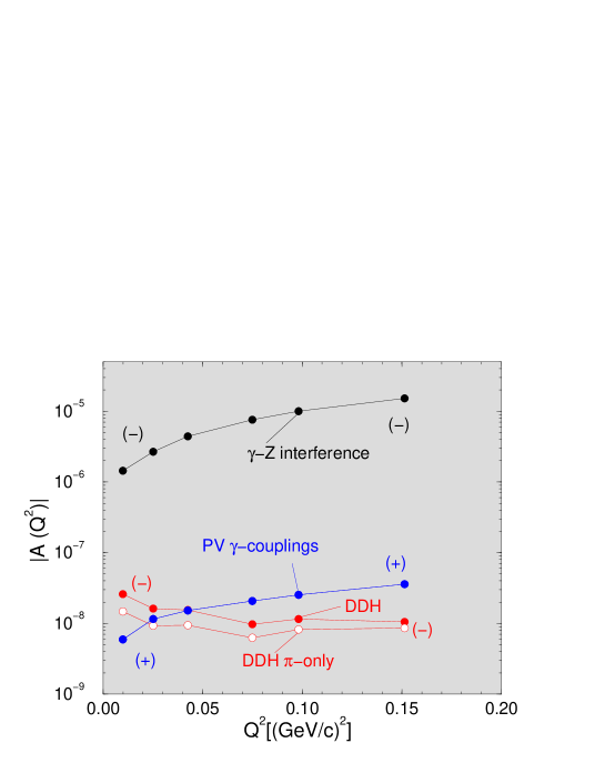
Figure 3: Calculation of the parity-violating asymmetry in deuteron electrodisintegration, from [81]. The process labeled “$\gamma$-$Z$ interference” is the dominant one-body contribution, the two labeled “DDH” are the contributions from the parity-violating NN interaction, and that labeled “PV $\gamma$-couplings” are the one-body anapole term plus two-body pion currents. The open (closed) symbols represent positive (negative) contributions to the asymmetry.

1.4 Related Observables: Spin, Mass, and Momentum

Strange quarks contributions to other observables, such as the nucleon’s spin, mass, and internal momentum distributions are well documented. The best source of information on strange quark unpolarized parton distribution functions, which are a measure of the fractional internal momentum distributions of the components of the quark-antiquark sea, is neutrino-induced dimuon production [84]. Neutrinos scattering from either an $s$ or $d$ quark in a nucleon produce a charm quark and $\mu^{-}$, and the charm subsequently decays producing a $\mu^{+}$. Tagging the events by simultaneous detection of the $\mu^{+}$ $\mu^{-}$ pairs provides a clean signature for the charm production. The probability of the charm production resulting from scattering from an $s$-quark is high, and the ($x$ or $\xi$) momentum distribution of the cross section can be directly related to the momentum distribution of the $s$-quark. Similar arguments apply for $\overline{\nu}$-$N$ scattering, where the $\overline{s}$ distribution is determined. The two distributions have generally been assumed to be the same and global data fits result in an integrated contribution of approximately 20% of the non-strange sea quark distributions or 2% of the total proton momentum [85]. More recently, the possibility of non-identical $s$ and $\overline{s}$ distributions is being investigated as a source of discrepancy between the value of $\sin^{2}\theta_{W}$ reported by the NuTeV collaboration [86] and the expectation from global fits to electroweak data [87]. While this issue remains to be resolved and new analyses to extract $s(x)$ and $\overline{s}(x)$ independently are underway, the integrated combination $s+\overline{s}$ appears to be relatively stable [84].

Another observable for which there is some indication of strange quark contributions is the proton’s mass, coming from a comparison of the isospin even $\pi$-nucleon scattering amplitude to the theoretical prediction for the quantity

$$\sigma\equiv\frac{1}{2M_{p}}\langle p|\hat{m}\left({\overline{u}}u+{\overline{d}}d\right)|p\rangle\$$ (24)

where ${\hat{m}}=\frac{1}{2}\left(m_{u}+m_{d}\right)$. The experimentally determined scattering amplitude is measured as a function of momentum transfer $q$ and extrapolated to $q^{2}=2m_{\pi}^{2}$, the Cheng-Dashen point [88], and is notated $\Sigma_{\pi N}$. In the absence of strange quark contributions, these two quantities should be equal. Extraction of the experimental value $\Sigma_{\pi N}$ has been plagued by discrepancies in the data and uncertainties in the extrapolation technique, and determination of $\sigma$ from theory is also problematic. A recent reanalysis using only scattering data relatively low threshold was carried out by [89], resulting in a value of $\Sigma_{\pi N}=71\pm 9$ MeV, somewhat higher than the value of 64$\pm$8 MeV previously determined in [90], but lower than that determined by an update [91] to the analysis in [90], of 90$\pm$8 MeV. Early determinations of the theoretical value led to $\sigma=45\pm 8$ MeV [92], but a more recent determination from lattice QCD results in $\sigma\sim 65$ MeV [93], not far from the most recent experimental determination. This would indicate no strange quark contribution to the proton’s mass. The variations over time of both the experimental $\Sigma_{\pi n}$ and the theoretical $\sigma$ demonstrate the difficulty of extracting a definitive determination of this quantity.

In the last decade a considerable body of data has accumulated on polarized deep-inelastic lepton-nucleon scattering (DIS), resulting in a well-determined measurement of polarized structure functions (for a recent review see [94]) from which one can deduce the contributions of sea quarks to the spin of both the proton and neutron. The proton’s spin can be formally written as

$$\frac{1}{2}=\frac{1}{2}\Delta\Sigma+L_{q}+J_{g}\,,$$ (25)

where the three terms are contributions from quark spin, quark orbital angular momentum, and gluon total angular momentum, respectively. The collective body of inclusive polarized lepton scattering data indicate that only a small fraction, approximately 20%, of the nucleon’s spin comes from the intrinsic spin of the quarks, the rest arising from $L_{q}$ and $J_{g}$. This result requires integrating the nucleon’s spin structure function over the full range of the quark momentum distribution, which is not completely measured. Extrapolations into the unmeasured region are thought to be under control. Assuming that SU(3) flavor is a good symmetry, the quark spin piece $\Delta\Sigma$ can be subsequently broken down into its contributions from $u$, $d$ and $s$ quarks, $\Delta\Sigma=\Delta u+\Delta d+\Delta s$, if the inclusive scattering data are combined with low energy nucleon and hyperon beta decay parameters, yielding the result that $\Delta s\sim-0.1$. A determination that does not require the assumption of SU(3) flavor symmetry can be found from semi-inclusive kaon production in spin-dependent DIS, and a result, $\Delta s=0.03\pm 0.03{\mathrm{(}stat.)}\pm 0.01{\mathrm{(}sys.)}$, using this technique has recently been reported by the HERMES collaboration [95], although integrated over only part of the quark momentum distribution.

The most direct measure of $\Delta s$ can in principle be made via elastic neutrino-proton scattering, a close analog of the parity-violation technique for extracting the vector form factors. The nucleon’s axial form factor as measured by neutrino scattering is free of the multi-quark radiative corrections that are present in electron scattering since they are coupled to a photon exchange between the lepton and hadron. Precise determination of the absolute cross section for elastic $\nu$-$p$ scattering is extraordinarily challenging due to the low cross sections and the difficulty in generating high-quality, high flux neutrino beams. An analysis of existing data [96] was carried out in [97]. The neutrino beam covered a broad range of momentum transfer centered about an incident neutrino energy of 1.25 GeV, so an assumption about the $Q^{2}$-dependence of the axial strange form factor was made. In addition, a strong correlation between the strange axial and strange vector form factors was seen. Recently, Pate [98] used the neutrino data again to demonstrate that $\Delta s$ can be better determined in a more global analysis that combines the neutrino data with the parity violation data, particularly with that expected to come from the G⁰ experiment which covers a similar range of momentum transfer (see section 3.3 below). The combined data will allow a first determination of the $Q^{2}$ dependence $G_{A}^{s}(Q^{2})$ ($\Delta s=G_{A}^{s}(0)$) over the range 0.45 - 0.95 (GeV/c)².

2 The SAMPLE Experiment

The main focus of this review is the program of experiments carried out by the SAMPLE collaboration, for which the primary goal has been to determine the contribution of strange quarks to the nucleon’s magnetic moment. The experiment was thus designed to detect scattered electrons in the backward direction at low momentum transfer, where contributions from $G_{E}^{s}$ are suppressed both because of kinematics and because the proton has no net strangeness. At the SAMPLE kinematics the axial term contributes approximately 20% to the asymmetry, and, while the strange quark piece of the axial term contributes negligibly, the uncertainties in the electroweak radiative corrections suggested that $G_{A}^{e}$ should be determined experimentally, requiring at least one additional measurement beyond elastic $e$-$p$ scattering. As discussed above, quasielastic scattering from deuterium has similar sensitivity to $G_{A}^{e}$, or at least to the dominant isovector component, but significantly lower sensitivity to $G_{M}^{s}$, and thus provided the second degree of freedom to independently determine $G_{M}^{s}$ and $G_{A}^{e}$.

The $e$-$p$ scattering measurements were carried out in 1998, followed by the first $e$-$d$ scattering experiment in 1999. The first analysis of the combined data sets indicated that, while strange quarks make up a small fraction of the proton’s magnetic moment, the measured isovector axial form factor ${G_{A}^{e}}^{(T=1)}$ was found to be in disagreement with the theoretical expectation. As a result, a second $e$-$d$ experiment was carried out in 2000/2001, at lower beam energy. The different kinematic conditions provided quite different experimental systematic uncertainties but similar sensitivity to ${G_{A}^{e}}^{(T=1)}$. A recently updated analysis of all three data sets has now brought both deuterium experiments into good agreement with theory, with little change to the extracted value of $G_{M}^{s}$  [1, 2]. In what follows we provide a summary of the experimental measurements along with the most recent updates to the data analysis and the final results for both $G_{M}^{s}$ and $G_{A}^{e}$ from the combined set of experiments. We begin, however, with a general discussion of polarized beam delivery for parity violation experiments, with the M.I.T.-Bates beam as our representative example.

2.1 Polarized Electron Beam and Beam Property Control and Measurement

Parity-violating electron scattering experiments require a polarized electron beam of high intensity and quality and the ability to control and accurately measure the properties of the beam. These requirements are driven both by the statistical and systematic error considerations of the experiments.

The current generation of parity-violation experiments typically measure asymmetries with a statistical error $\sim$0.1-1 ppm. Statistical errors of this precision require luminosities $\sim 4\times 10^{38}\ \hbox{cm}^{-2}\hbox{s}^{-1}$ for reasonable ($<$ 1000 hours) running times. Currently available high power hydrogen and deuterium targets have typical target lengths in the 15-40 cm range, which implies the need for 40 - 100 $\mu$A of 40-80% polarized electron beam. Modern polarized electron sources have achieved these requirements. The most convenient way to quantify the impact of polarized electron source capabilities on the experiments’ statistical error is in terms of the figure-of-merit, $P^{2}I$. Here, $P$ is the electron beam polarization and $I$ is the beam current. For a given running time it is desirable to maximize this figure-of-merit to achieve the minimum statistical error.

The impact of beam property control and measurement capabilities on systematic errors enters primarily in two ways. First, one must measure the beam polarization accurately and ensure that it is longitudinal to the required precision. Examples of polarimeters and techniques to accomplish this are discussed in later sections. Second, one must control and measure the helicity-correlated properties of the beam and properly assess their impact on the measurement. In an ideal parity-violation experiment, no property of the beam changes when its helicity is reversed; in reality, many properties of the beam such as position, angle, and intensity are observed to change. This can cause a false asymmetry:

$$A_{false}=\sum_{i=1}^{N}\frac{1}{2Y}\frac{\partial Y}{\partial P_{i}}{\Delta P_{i}}.$$ (26)

Here, $Y$ is the detector yield, $P_{i}$ respresents beam properties including position, angle, intensity, and energy, and $\Delta P_{i}=P_{i}^{+}-P_{i}^{-}$ is the helicity-correlation in those beam properties. The false asymmetries are typically reduced by construction of a symmetric detector (to minimize $\partial Y/\partial P_{i}$) and active feedback to reduce helicity-correlated beam properties (to minimize $\Delta P_{i}$). Any residual helicity-correlations in the beam properties are then corrected for by regular measurement of the dependence of the detector yield on a given beam property (${\partial Y/\partial P_{i}}$) and then correction of the measured asymmetry: $A_{corr}=A_{meas}-A_{false}$. This corrections procedure is used by all of the current generation of parity violation experiments

The requirements on the beam property measurement and control devices are set by the corrections procedure. The beam properties are measured and averaged continuously and recorded at every helicity reversal. The beam property differences $\Delta P_{i}$ typically have a nearly Gaussian distribution, with a centroid $\overline{\Delta P_{i}}$ and a standard deviation $\sigma_{\Delta P_{i}}$. The centroid represents the average helicity-correlated beam property difference for that parameter, and it must be kept small enough so that the corrections to the asymmetry are typically only a few percent of the measured asymmetry. In practice, active feedback on the beam properties is necessary to achieve this. The standard deviation has contributions from the random fluctuations in that beam property at the helicity-reversal frequency and also the finite measurement precision of the beam monitoring equipment. The error on the determination of the centroid is $\sigma_{\Delta P_{i}}/\sqrt{N}$, where $N$ is the total number of difference measurements. Thus, the standard deviation $\sigma_{\Delta P_{i}}$ must be kept small enough to allow accurate measurements of the centroid in a reasonable time period, both for feedback purposes and in determining the error on the corrections procedure.

Many of the polarized source techniques and beam control and measurement methods needed for current experiments were incorporated in the pioneering parity-violating deep inelastic scattering experiment of Prescott and collaborators [99] at SLAC in the late 1970’s. Techniques were further refined and developed at MIT-Bates [100] and Mainz [101] over the next decade. In the remainder of this section, we focus our discussion on the polarized beam techniques and the experience of the SAMPLE collaboration at MIT-Bates in the late 1990’s as a representative example.

2.1.1 MIT-Bates Polarized Electron Source

In this section, we describe some important details of the MIT-Bates polarized electron source, starting with a discussion of several features that are common to all polarized electron sources. The polarized electrons are produced via photoemission from a specially prepared gallium aresenide (GaAs) photocathode. The special preparations include heat cleaning of the photocathode and activation of the crystal via deposition of cesium and an oxidizer (O₂ or NF₃) to create a negative electron affinity surface. The negative electron affinity surface allows the electrons optically excited to the conduction band to escape the cathode. There are two general types of GaAs photocathodes in use: bulk and strained GaAs. Due to the band structure of the GaAs crystal, the photoemitted electrons can be emitted with a theoretical maximum of 50% polarization when 100% circularly polarized photons are incident on bulk GaAs. Strained layer GaAsP photocathodes break an energy level degeneracy in the valence band; in these photocathodes, emitted electron polarizations of 100% are theoretically possible. In practice, typical polarizations of 35-40% are achieved with bulk GaAs crystals, and 70-85% for strained layer GaAsP crystals. Bulk GaAs crystals can have quantum efficiencies (QE) $>\sim$1%, while strained GaAsP crystals typically have much a lower QE. Lasers of various types are used to provide the incident light flux necessary to achieve the desired electron beam currents.

A schematic of the important components of the MIT-Bates polarized electron source, which was used to provide beams for the SAMPLE experiment, is shown in Figure 4. The MIT-Bates Linear Accelerator is a pulsed machine, with typically 35 $\mu$s duration electron beam pulses at 600 Hz. This low duty factor implies a peak current that is about one to two orders of magnitude higher than that needed for comparable average beam currents at CW electron accelerators like those at Jefferson Laboratory or Mainz. The commercial laser solution adopted at MIT-Bates consisted of an argon ion laser pumping a Ti:Sapphire laser. Thermal lensing effects in the Ti:Sapphire crystal were minimized by chopping the argon ion laser pump beam with a phase locked electro-mechanical chopper. The typically available peak powers of about 3.5 W with this system required that the SAMPLE experiment use bulk GaAs crystals with typical beam polarizations of $\sim$37% for production running. The quantum efficiency of the higher polarization strained GaAsP crystals was too low to achieve the desired 40 $\mu$A average beam current. Under typical running conditions with this laser and a bulk GaAs crystal, the MIT-Bates polarized source peak currents were 4-6 mA, with average currents of $\sim$120 $\mu$A before chopping of the electron beam in the injector, and $\sim$40 $\mu$A on the SAMPLE target. The source produced about 400 C of polarized electron beam on target over the course of the three SAMPLE production runs.

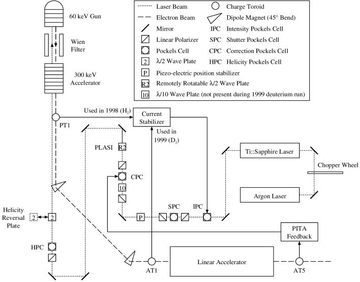
Figure 4: A schematic of the MIT-Bates Linear Accelerator polarized electron source.

The time structure of the laser beam was matched to that of the accelerator with the shutter Pockels cell (SPC) system, consisting of a Pockels cell between crossed linear polarizers to allow for electro-optic intensity modulation. Under normal operating conditions, this system produced 25 $\mu$s duration laser pulses at 600 Hz. The helicity of the laser beam was defined with the helicity Pockels cell (HPC) system, consisting of a linear polarizer followed by a Pockels cell set to quarter-wave voltage. Rapid polarization reversal is critical in parity experiments to reduce sensitivity to slow drifts in detector and beam properties. The polarization sequence used in the MIT-Bates polarized source is shown in Figure 5. The electron beam bursts are sorted into “timeslots” depending on their phase in the 60 Hz power line cycle. Since the accelerator operating frequency is 600 Hz, there are 10 such timeslots. For each of the 10 timeslots, the polarization is selected pseudo-randomly, referred to as the “NEW” sequence. It is followed by ten states that are the complement of the previous ten, referred to as the “COMP” sequence. Asymmetries and beam parameter differences are formed from the “pulse-pair” defined by the NEW and COMP states for a given timeslot. Analyzing the data in this way removes the effect of the dominant 60 Hz power line noise on the experiment. In addition to reversing the beam helicity with this technique, an insertable half wave plate, located downstream of the HPC, was used to manually reverse the beam helicity without changing the state of the HPC or the helicity control electronics. In the SAMPLE experiment this was carried out approximately every other day, and was an important systematic check to assure immunity of the experiment’s detector electronics to the HPC high voltage and related helicity signals.

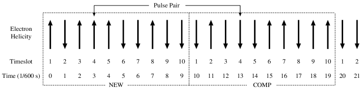
Figure 5: Polarization sequence used in the MIT-Bates polarized source. The first ten states are chosen pseudo-randomly, followed by ten states that are the complement of the previous ten.

A particular aspect of the MIT-Bates polarized source that was important for SAMPLE running was the intensity stabilizer system. This was an active feedback system that reduced the random fluctuations in the laser intensity. The system consisted of a Pockels cell electro-optic intensity modulator (IPC). The electron beam current was measured at a point early in the accelerator. The difference between it and a reference signal was amplified and applied to the intensity modulator in order to stabilize the output beam current. This system suppressed instabilities in laser intensity, extraction efficiency, and the first stage of the electron beam transport system. The system had a bandwidth of 1 MHz which allowed it to stabilize the beam current within the 35 $\mu$sec beam pulses. The typical observed stability of the beam current at the 600 Hz helicity flip frequency was $\sim$ 0.2 - 0.5%.

A more complete description of the MIT-Bates polarized electron source can be found in reference [102].

2.1.2 Electron Polarimetry and Spin Transport at MIT-Bates

Two electron beam polarimeters were used during the SAMPLE experiment to precisely measure the longitudinal component of beam polarization and for spin transport measurements to manipulate the spin to a longitudinal state. The primary apparatus was a Møller polarimeter upstream of the SAMPLE detector, and this was augmented by a transmission polarimeter in an injection chicane early in the accelerator where the beam energy was 20 MeV. The Møller polarimeter measurements were typically done every 3 days, while the transmission polarimeter measurements, which were significantly faster, were carried out daily.

The Møller polarimeter is shown in Figure 6. The device was located about 26 m upstream of the SAMPLE target. The electrons were scattered from a Supermendur foil (49% Fe, 49% Co, 2% Va), which could be rotated to any desired target angle. The target chamber was instrumented with two sets of orthogonal Helmholtz coil pairs to allow for target polarization both in the scattering plane and perpendicular to it. The analyzing power for Møller scattering is maximum at $\theta_{CM}=90^{\circ}$, so the collimator was set to accept scattered electrons at that angle. The spectrometer consisted of two dipoles that gave point-to-point focusing in both dimensions at a fixed energy of 200 MeV. The scattered electrons were detected in a Lucite Čerenkov counter. The resulting signals were integrated over the ($\sim 25-35$ $\mu$s duration) beam burst.

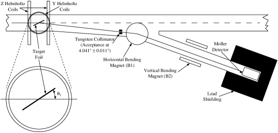
Figure 6: Schematic of the SAMPLE Møller polarimeter.

The performance of the Møller polarimeter satisified the needs of the SAMPLE experiment. The Møller peak was observed by scanning the spectrometer over a large enough range to include the momentum of the scattered Møller electrons and backgrounds from nuclear scattering and other processes. Typical observed signal to background ratios were about 5:1. Yield and asymmetry results from a typical scan of the spectrometer are shown in Figure 7. The relative statistical error on the polarization in a 20 minute measurement was about 2%. The relative systematic error from all sources was estimated to be about 4.2%, with the dominant component of this coming from the 3.2% uncertainty in the signal to background extraction. The correction for the Levchuk effect [103] due to scattering from bound electrons was estimated to be about 2.8% from a Monte Carlo simulation of the apparatus.

Figure 7: A typical momentum scan of the Møller spectrometer. The plots show the yield and asymmetry as a scan through the Møller peak is performed.

Typically, a Møller measurement could take up to 2 hours due to the need to retune the beam so that it was focused on the Møller target, and then restore regular running conditions afterwards. It was desirable to have another polarimetry technique with reduced overhead and which could be done more frequently since the polarization tends to vary with time. Empirically, there is a trend for the polarization to increase as the GaAs photocathode quantum efficiency decreases. During the two deuterium runs, more rapid polarization measurements were carried out with a transmission polarimeter.

The transmission polarimeter was located in the middle of the input chicane of the MIT-Bates accelerator, at a point where the beam energy was 20 MeV. A schematic of the polarimeter is shown in Figure 8. During normal operations, the beam would pass straight through, but the beam could be quickly deflected into the chicane for polarization measurements when desired. The whole process, including restoring regular operations, could be completed in 10 minutes. The transmission polarimeter consisted of a BeO radiator in the middle of the chicane. Bremsstrahlung emitted from the radiator was detected in a transmission style photon Compton polarimeter. It consisted of two scintillation counters with an iron electromagnet in between them. The longitudinal component of the electron beam spin was transferred to the bremsstrahlung. The circular polarization of the bremsstrahlung was detected via the spin-dependent absorption in the polarized iron and the resulting asymmetry in the transmitted flux. The absolute analyzing power of such a device is difficult to calculate directly. Instead, it was determined empirically by cross calibrating with the SAMPLE Møller polarimeter. The transmission polarimeter functioned very well as a relative polarization monitor during the run. It typically delivered beam polarization measurements with $<1\%$ relative statistical error in about 2 minutes of measurement time. The cross-calibration relative to the Møller polarimeter was very stable with respect to time; results are shown in Figure 9.

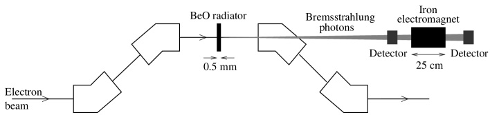
Figure 8: A schematic view of the MIT-Bates transmission polarimeter.

Figure 9: The ratio of the polarization from the Møller polarimeter and transmission polarimeter (in arbitrary units) versus day shown over the course of 60 days. The cross-calibration was very stable during the entire period.

For the SAMPLE experiment, it was important to ensure that the transverse beam polarization components were small, because there exists a parity-conserving left-right analyzing power that can result in a false asymmetry if the detector geometry is not perfectly symmetric about the beam line. A careful spin transport procedure was developed for the experiment, used both to minimize the transverse polarization for regular running and also to maximize the transverse polarization for dedicated runs to measure the sensitivity of the experiment to it. The SAMPLE beamline was at a 36.5^∘ bend relative to the main accelerator, which resulted in a precession of the electron spin orientation, due to its (“$g-2$”) anomalous magnetic moment, by 16.7^∘ at 200 MeV. This was compensated for by pre-rotating the electron spin in the 60 keV region of the accelerator with a Wien filter (a device with crossed electric and magnetic fields). However, there also are many focusing solenoid magnets located in the low energy end of the accelerator which would cause the spin to precess about the beam axis, and they had to be set to insure that the net precession put the spin back into the bend plane of the accelerator. A procedure was developed to independently calibrate the effect of the Wien filter and accelerator solenoids on the spin so that they could be used to reproducibly set the desired spin direction. The procedure [104] made use of the SAMPLE Møller polarimeter, which was equipped with a rotatable target ladder, allowing the target to be polarized with components both perpendicular and parallel to the beam direction in the bend plane. In terms of all the relevant angles, the asymmetry between left and right-handed electrons in the Møller apparatus can be written as:

$$A\;\> = \;\>{(P^{B}P^{T}/9)}[{1/(1+B/S)}]\times$$

$$\;\>[(7\cos\theta_{T}\sin\theta_{g}-\sin\theta_{T}\cos\theta_{g})\sin\theta_{W}\langle\cos\phi\rangle-(7\cos\theta_{T}\cos\theta_{g}+\sin\theta_{T}\sin\theta_{g})\cos\theta_{W}]$$

Here $P_{T}\sim 0.080$ and $P_{B}\sim 0.35$ are the target and beam polarizations, respectively, and $S/B$ is the signal to background ratio of the detected scattered electron yield. The angles are the Wien precession angle $\theta_{W}$, the out-of-plane precession angle $\phi$, the angle between the plane of the target foil and the beam direction $\theta_{T}$, and the $g-2$ spin precession angle $\theta_{g}$ (16.7^∘ for our beamline at 200 MeV). At a specific target angle ($\tan\theta_{T}=7\tan\theta_{g}$), the first term involving $\phi$ in equation 2.1.2 is eliminated. The second term involves only the Wien angle $\theta_{W}$, so the Wien filter can be calibrated directly, independent of the settings of the accelerator solenoids. Results of such a calibration are shown in Figure 10. The Wien filter calibration is then used to precisely set $\theta_{W}=90^{\circ}$, which eliminates the second term in equation 2.1.2. The target is then set at an angle ($\theta_{T}=-25.6^{\circ}$ for our $\theta_{g}$) which maximizes the amplitude of the first term. Then the dependence of the angle $\phi$ on solenoid current can be determined, resulting in a solenoid calibration as shown in Figure 10. The calibrations obtained from this procedure could be used to set the spin angles with a precision of $\delta\phi=\pm 5^{\circ}$ and $\delta\theta_{W}=\pm 1^{\circ}$, allowing the overall spin direction to be longitudinal to within $2^{\circ}$. In the SAMPLE experiment this level of alignment was sufficient to ensure that any contribution for the parity-conserving left-right analyzing power is negligible in the SAMPLE experiment.

Figure 10: In the top figure a calibration curve for the Wien filter is shown as the Møller asymmetry as a function of the Wien filter electric field setting. In the lower figure is a result of the calibration of the accelerator solenoids resulting from the Møller asymmetry as a function of the net deviation of the solenoid magnet currents from their nominal settings.

2.1.3 Beam Property Measurement and Control

As outlined in Section 2.1, measurement and control of beam properties is a critical part of parity violation experiments. In this section, we describe how the beam properties for the SAMPLE experiment were measured and what feedback systems were implemented in order to control the beam properties at the desired level. Figure 11 shows the critical elements that were used for beam measurement and control in the SAMPLE experiment. The beam properties of interest are the beam energy, position and angle at the SAMPLE target, and beam intensity. Feedback systems to reduce the 60 Hz power line noise in the beam energy and helicity-correlations in the beam position and intensity were implemented.

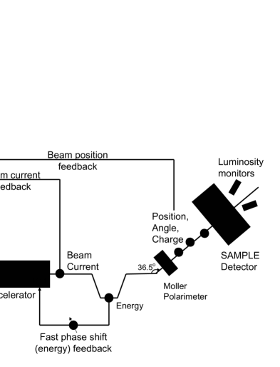
Figure 11: Schematic representation of the critical elements for beam measurement and control in the SAMPLE experiment. The beam current and beam position feedback systems reduce the helicity correlated charge asymmetry at the end of the accelerator and the helicity-correlated beam position differences upstream of the SAMPLE detector.

The beam energy was measured at the point of highest dispersion in the center of a magnetic chicane, a diagram of which is shown in Figure 12. The dispersion at this point was $35\ \hbox{mm}/\%$, and the beam energy was determined from a measurement of the beam position at that location. The dominant fluctuations in the beam energy were correlated with 60 Hz variations in the electrical power. This was potentially problematic for the SAMPLE experiment because when the variations in the energy were significant enough to cause tails of the beam to scrape on an energy defining collimator, a significant background in the SAMPLE detector could be observed.

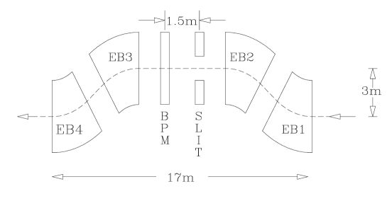
Figure 12: Schematic diagram of the MIT-Bates energy chicane showing the BPM, the energy limiting slits, and the four dipole magnets that define the magnetic chicane.

To reduce this variation, a feedback system was implemented [105], in which the beam energy for each of the ten phases (“timeslots”) of the 60 Hz line cycle during the 600 Hz running was measured independently. Corrections were then applied to force the beam energy to be the same for all ten timeslots, thus greatly reducing the 60 Hz fluctuations. The energy adjustments were made by slightly detuning one of the accelerator klystrons away from its maximum and using a fast phase-shifting device to compensate for the 60 Hz variations. Results of this system are shown in Figure 13. The 60 Hz variation in the beam energy was reduced by an order of magnitude, and this system was also very effective in suppressing slow ($\sim$ seconds or longer) beam energy drifts of thermal origin.

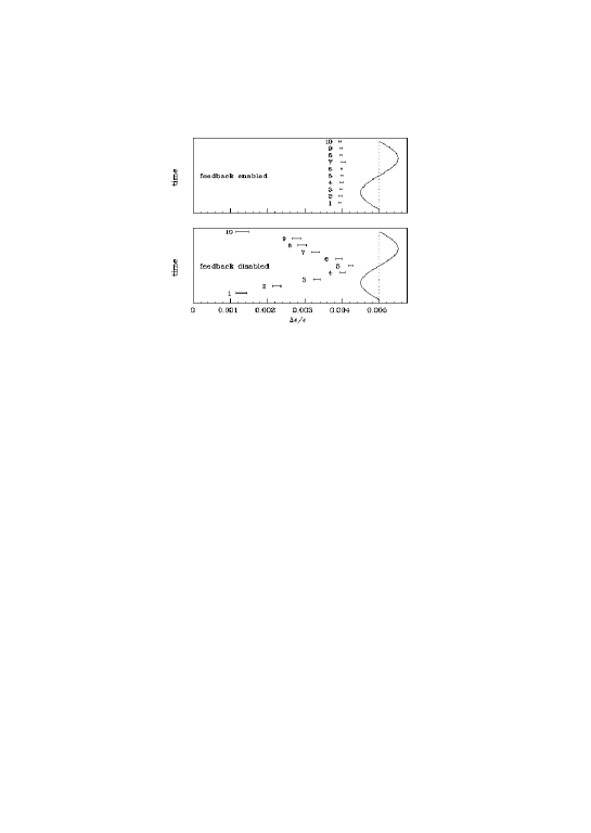
Figure 13: Fractional energy change as a function of phase of the 60 Hz line cycle (“timeslot”). The lower (upper) panel shows the behavior of the beam with the energy feedback system disabled(enabled). The 60 Hz AC line voltage is superimposed to set the time scale.

The beam position and angle at the SAMPLE target were measured with a pair of microwave cavity position monitors, similar to those employed at SLAC [106]. These monitors give a signal that is proportional to the product of beam position and beam charge. The beam charge was measured using a nearby toroid monitor, the position then resulting as the ratio of the two signals. Two (XYQ) monitors were located 4 and 8 meters upstream of the target so that both position and angle could be measured in the horizontal and vertical directons. The monitor signals were integrated and digitized every 25 $\mu$s beam burst, and helicity-correlated “pulse-pair” differences were formed to continuously measure the difference of the average beam position for the left and right-handed helicity states of the electron beam. Typical standard deviations for these distributions were $\sim$20-60 $\mu$m, where the dominant contribution came from the random fluctuations in the beam position at the reversal frequency. The intrinsic resolution of the monitors was small compared to this.

Under normal conditions, the helicity-correlations in the beam position were large enough that they would lead to large false asymmetries in the experiment. These correlations had their origin in the optical elements in the laser beam path, as determined from extensive study. The laser beam position was measured with a photodiode segmented into four quadrants. There were two general classes of effect: direct effects from the helicity-defining Pockels cell and secondary effects due to spatial polarization gradients in the laser light circular polarization created by the Pockels cell. The direct effects were observed as helicity-correlated laser beam angular steering and position shifts when the high voltage on the Pockels cell was reversed. Secondary effects were due to spatial gradients in the circular polarization quality across the laser spot. When the laser beam interacted with optically analyzing surfaces (like mirrors) this would cause a spatially dependent light transmission which appeared as a position shift of the laser beam. The secondary effects were minimized by making the HPC the last optical element in the system, right before the vacuum window into the electron gun. The direct effects were minimized by careful alignment of the Pockels cell, but the residual effects were still large enough that a dedicated feedback system to minimize helicity-correlated position differences was necessary.

The position feedback system [107] was implemented using a plate of optical glass in a mount with piezoelectric (PZT) steering pads, placed directly in the laser beam path. For a small tilt angle, $\theta$, of the glass with respect to the laser beam there is a pure translation of the laser beam $\delta=(1-\frac{n_{a}}{n_{g}})t\theta$, where $n_{a(g)}$ is the index of refraction of the air (glass) and $t$ is the thickness of the glass. The piezoelectric pads could be driven at the helicity reversal frequency (600 Hz), so it was possible to use this system to correct for the helicity-correlations. In practice, the electron beam position differences were typically measured over a period of eight hours, resulting in a precision of about 25 nm. The PZT system would then be adjusted to null the position differences at the SAMPLE target. Some typical position differences with PZT feedback on and off are shown in Figure 14. Typical position differences with no feedback were $\sim$50-200 nm, and with feedback implemented, these position differences were reduced by an order of magnitude.

Figure 14: Some typical position differences measured in one hour runs with the helicity-correlated position feedback system on and off.

The net beam charge in each beam pulse was measured non-invasively with monitors located upstream of the SAMPLE target. Each monitor consisted of an iron toroid wrapped with wire to detect the change in magnetic flux as the beam passes through the center. Helicity-correlations in the beam intensity can affect the experiment in two ways. The first is through non-linearities in the detector phototubes or electronics. After the integrated detector signal is normalized to the beam charge, any non-linearity will show up as a dependence of this normalized yield on beam current. So, a nonzero beam charge asymmetry would lead to a false asymmetry. The second, and more significant effect for SAMPLE, resulted from the beam loading of the MIT-Bates accelerator, or dependence of beam energy on the beam intensity, which could result in helicity-correlated energy shifts. A feedback system (called the CPC, for corrections Pockels cell) was thus implemented to reduce the helicity-correlated intensity asymmetry. The origin of the intensity asymmetry was found to be, as with the position differences, in the helicity Pockels cell (HPC). The HPC produces imperfect circularly polarized light resulting in small residual linearly polarized components in the two states. These two states then have different transmission coefficients when they interact with downstream optical elements, thus resulting in an intensity asymmetry. The CPC consisted of linear polarizers with the same orientation sandwiching a Pockels cell operating at low voltages. The CPC could be driven at different voltages for the two helicity states, so it acted as a helicity-correlated intensity modulator. The feedback was carried out by measuring the intensity asymmetry in a beam charge monitor at the end of the accelerator. The measurement time was typically about 3 minutes, allowing the intensity asymmetry to be determined with a precision of $\sim$ 10-20 ppm. The CPC control voltage was then adjusted to null the intensity asymmetry. Typical results with the CPC feedback system on and off are shown in Figure 15. Without feedback the charge asymmetries were typically 30-70 ppm, but with feedback they were suppressed by more than an order of magnitude.

Figure 15: Typical intensity asymmetries measured in one hour runs with and without the CPC feedback system running.

The helicity-correlated position and intensity feedback systems described here were used for all three of the data-taking runs of the SAMPLE experiment. Results for the helicity-correlated beam properties averaged over an entire major run consisting of about 800 hours are shown in Table 3. The resulting values were such that the corrections to the data for false asymmetries were less than the statistical uncertainty of the measured parity-violating asymmetries.

Beam property	Run-average helicity correlation
$\Delta X$	$7.6\pm 2.3\ \hbox{nm}$
$\Delta Y$	$-1.9\pm 1.4\ \hbox{nm}$
$\Delta\theta_{X}$	$-0.6\pm 0.1\ \hbox{nr}$
$\Delta\theta_{Y}$	$-0.9\pm 0.3\ \hbox{nr}$
$\Delta E$	$0.14\pm 0.02\ \hbox{eV}$
$A_{I}$	$-0.04\pm 0.13\ \hbox{ppm}$

Table 3: Helicity-correlated beam properties averaged over about 800 hours for the 1998 SAMPLE LH₂ running period.

2.2 The SAMPLE Experimental Setup

A schematic of the SAMPLE apparatus is shown in Figure 16. The polarized electron beam was incident on a 40 cm long aluminum cell filled with liquid hydrogen. The scattered electrons exited the target and passed through a 3.1 mm thick hemispherical aluminum scattering chamber lined with 2.5 mm of Pb before entering the volume of air that served as a Čerenkov medium for the detector. The detector, the design of which was based on a similar detector used at the Mainz Laboratory [101], consisted of ten ellipsoidal mirrors that focused Čerenkov light onto ten 8-inch diameter photomultiplier tubes. This constituted an azimuthally symmetric detector system with a solid angle of approximately 1.5 sr, covering scattering angles between 138^∘ and 160^∘. The photomultiplier tubes were encased in Pb cylinders to minimize background from electromagnetic radiation, and remotely controlled shutters in front of the phototubes allowed measurement of non-light producing background entering the Pb cylinders. The detector components and target were encased in a light-tight box and all metal surfaces were blackened in order to minimize background from stray light. In the two deuterium experiments, borated polyethylene shielding was added between the target and photomultiplier tubes to reduce background from photo-produced neutrons in the target.

Due to the high count rate in the detector system (more than 10⁸ s^-1), the detector signals were integrated over the 25 $\mu$s long beam pulse of the Bates beam. The energy threshold for Čerenkov production in air for electrons is 20 MeV, thus the measured yield in the detector was the integral of all scattered electrons and positrons above this value. As a result, background in the detector had to be measured in dedicated runs. The non-light producing background was measured regularly throughout the experiments using the phototube shutters. In the light portion of the signal, an additional component, approximately 15%, was due to scintillation light produced in the air. This component was measured at reduced beam current by placing a set of auxiliary detectors behind each mirror, requiring a coincidence between the auxiliary detectors and the phototubes, and analyzing the pulse-height spectrum of the phototube signals. In the later experiments an alternative method for determining the scintillation component at high beam current was developed, which consisted of measurement of the phototube yields with the mirrors covered. Both methods are discussed in more detail below.

The cryogenic target system [108] was designed to rapidly flow liquid hydrogen or deuterium through the 40 cm long cell in order to minimize potential effects of beam heating on the target density. The cryogenic fluid had to be able to absorb the approximately 500 Watts of power deposited by the beam with negligible changes in density on the time scale of a single asymmetry measurement (16 ms). The target was cooled with a helium gas refrigerator that delivered 12 K coolant through a counterflow heat exchanger and was capable of removing up to 700 Watts of bulk heating. A Chromel ribbon resistive heater immersed in the target fluid was operated in a feedback loop with the beam current to maintain a constant heat load on the target that kept the average temperature of the target constant to within 0.5 degrees. Measurements to look for fluctuations in target density were carried out in dedicated periods during each experiment and they were found to be negligible compared to the statistical fluctuations of the measured yield.

Small Čerenkov detectors consisting of lucite attached to two inch photomultiplier tubes were located downstream of the SAMPLE target at a scattering angle of $\sim 7.5^{\circ}$. Typically, two to four of these luminosity monitor detectors were used at various locations about the azimuth. Each detector had a factor of three smaller statistical error than the combination of the ten main SAMPLE detectors, and as a result they were a sensitive monitor of potential fluctuations in target density. These monitors were also used as a null asymmetry monitor. The detected signal in these monitors was primarily from very forward scattered electrons at low momentum transfer and/or from electromagnetic showers, for which the expected asymmetry is significantly smaller than the main parity-violating signal of the experiment.

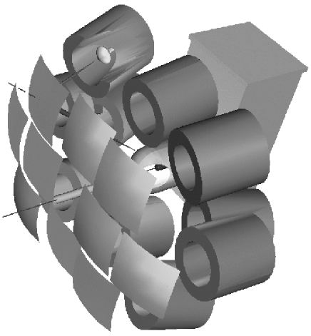
Figure 16: Schematic of the SAMPLE apparatus. Portions of the scattering chamber and lead shielding have been cut away for clarity.

The raw photomultiplier tube signals were sent through current-to-voltage amplifiers prior to integration over the 25 $\mu$s beam pulse. The integrated voltages were dithered with a small additional random voltage (which was subtracted in analysis) before being digitized in order to remove the potential effects of differential nonlinearities in the 16-bit analog-to-digital converter modules used in the readout system. The data stream was read out during the 1.5 ms between beam bursts so the data acquisition system was free of deadtime. The data stream included not only the ten photomultiplier tubes but also beam current and position monitors along the accelerator that would indicate potential helicity correlated beam properties concurrent with the measurement. The helicity of the beam was flipped randomly in a sequence of ten beam pulses, reversed for the next ten pulses, and then paired to form ten asymmetry measurements. Approximately one in 39 beam pulses was blanked to keep track of potential baseline shifts, and the beam helicity was reported to the data stream after digitization of the analog signals, and in a symmetric fashion, in order to avoid electronic cross talk or potential helicity correlated baseline shifts. The ten “time-slot” asymmetries were averaged together, and then averaged over a one-hour period.

2.3 Data Analysis

In the first pass through the data analysis, the raw detector asymmetries were computed, as well as each detector’s sensitivity to the measured beam properties using the natural, helicity-uncorrelated motion of the beam over a one-hour period. In a second pass through the analysis, the measured asymmetry was corrected for false asymmetries arising from helicity-correlated beam motion using a linear regression procedure on the detector yields on a pulse-by-pulse basis. The linear regression accounts for correlations between parameters as well as correlations with the detector yields, and the procedure is mathematically equivalent to subtraction of a false asymmetry arising from the helicity correlated beam properties.

With one exception (see below), the corrections made to the asymmetry were always less than its statistical uncertainty. The same corrections procedure was also applied to the luminosity monitors. Due to the small momentum transfer of the accepted events in these monitors, the expected asymmetry was smaller than the precision with which it was measured, so these monitors could be used to assess performance of the corrections procedure in eliminating false asymmetries and to quantify the errors assigned to the corrections procedure. After the corrections were applied to the data, the detector asymmetry values were sorted based on state of the insertable half wave plate, which was reversed every few days. In Figure 17, the expected reversal of the sign of the measured asymmetry is clearly seen in the data. The net correction, averaged over ten mirrors, applied to the hydrogen (raw asymmetry) data was 0.07 ppm with an assigned systematic uncertainty of 0.05 ppm. The systematic uncertainty was estimated by assuming that all of the residual asymmetry of the luminosity monitors, measured to be 0.05$\pm$0.05 ppm, was due to any error in the corrections procedure. It should be re-emphasized that the corrections were computed and applied on a detector-by-detector basis, although the correction varied little from one detector to the next. The equivalent quantity in the 200 MeV deuterium run was 0.07 ppm with an assigned uncertainty of 100% of the correction. While in each of these runs the contribution from beam helicity correlations to both the asymmetry and its systematic uncertainty are very small, in the third SAMPLE run, the corrections were larger due to a significant helicity correlated transmission asymmetry of the beam. This issue is described in more detail below.

Figure 17: Averaged asymmetries for each state of the half wave plate are shown as a function of time. The asymmetries in this plot is the measured asymmetry of the sum of the 10 photomultiplier tube signals corrected for helicity-correlated beam properties with the linear regression procedure described in the text. The solid lines show the overall average value of the asymmetry in each of the two states, IN (triangles) and OUT (circles). It should be noted that this phototube sum signal is not the quantity used to construct the final experimental asymmetry, rather the statistically weighted average of the ten phototube signals was used.

Once the measured asymmetry has been corrected for false asymmetries due to the beam, other dilution factors and potential sources of yield in the asymmetry that arise from physics processes other than elastic $e$-$p$ scattering must be accounted for. The largest dilution factor is that due to the beam polarization, which was 35-40% in each of the three experiments. The remaining corrections can be summarized in the following expression:

$$A_{exp}=\frac{R_{c}}{P_{B}f_{l}f_{c}\left(1-f_{\pi}\right)}\left[A_{O}-\left(1-f_{l}\right)A_{C}-f_{\pi}A_{\pi}\right]$$ (28)

where $P_{B}$ is the electron beam polarization, $R_{c}$ is an electromagnetic radiative correction due to emission of bremsstrahlung, $f_{l}$ is the fraction of the yield due to light incident on the photomultiplier tubes, $f_{c}$ is the fraction of the light-producing signal due to Čerenkov radiation, and $f_{\pi}$ is the fraction of the Čerenkov light due to $\pi$-production in the target. The quantity $A_{O}$ is the asymmetry measured under normal running conditions, after corrections for beam helicity correlations, and $A_{C}$ is the asymmetry measured with shutters in front of the photomultiplier tubes to block incident light. In the first two SAMPLE experiments, approximately one quarter of the data taking was devoted to these “shutter-closed” measurements. In the third, this fraction was reduced to 10%, but additional measurements of the CLOSED asymmetry were made by enhancing its contribution with a piece of plastic scintillator placed in front of each photomultiplier tube. The light fraction $f_{l}$ was determined with high precision from these data and contributed a negligible uncertainty to the dilution corrections. While in each of the three measurements the average background asymmetry was consistent with zero, mirror-by-mirror variations resulted in the need to handle this contribution differently in the three experiments, as discussed in more detail below.

In each of the three SAMPLE experiments the Čerenkov fraction $f_{c}$ was determined with a set of dedicated measurements in which the beam current was reduced to a level such that individually scattered electrons could be counted and the pulse height distributions of the photomultiplier signals recorded. One in ten beam pulses contained enough beam charge that statistically meaningful integration measurements could also be made in order to monitor that beam properties were comparable to those during normal high-current running (these pulses were used only for monitoring beam properties and not included in the data stream.) Identification of the Čerenkov component of the pulse-height spectrum was made by requiring a coincidence between a plastic scintillator placed behind each mirror and its corresponding photomultiplier tube. The Čerenkov fraction was then defined to be the integrated yield in the coincidence pulse-height spectrum relative to the yield in the singles spectrum, after normalization to integrated beam charge and correction for dark current contributions and dead time effects. An additional correction was made to the coincidence pulse-height spectrum due to the fact that the scintillators covered only the central portion of the mirrors. Under normal integration running conditions and in the singles event pulse height distribution, the spectrum of Čerenkov photons per incident electron is slightly distorted because the edges of the mirror do not have full acceptance of the scattered electron’s Čerenkov cone. This distortion of the Čerenkov spectrum was simulated and resulted in an enhancement of the measured $f_{c}$ by 5%. Figure 18(a) shows a typical spectrum of coincidence count rate as a function of time where the 25 $\mu$s beam pulse can be clearly identified. In Figure 18(b) the pulse height spectra for singles and coincidence events are shown for one detector.

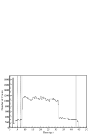
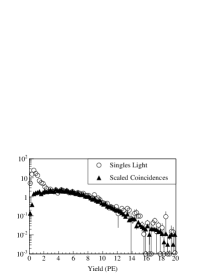
Figure 18: (a) Coincidence event timing spectrum during low-current measurement of the Čerenkov fraction $f_{c}$, showing the period of time prior to beam delivery (dashed lines) used for dark rate determination. (b) Pulse height spectra for the singles (circles) and coincidence events (diamonds) after correction for dark current, dead time, and the edge-effects of the mirrors.

In the two deuterium experiments an alternate method of determining $f_{c}$ was developed that did not require reducing the beam current. Covers were placed over the mirrors in order to determine what fraction of the light yield in a given phototube did not involve direct reflection off of its corresponding mirror. This method was combined with a simulation of scintillation production in the air between the mirrors and photomultiplier tubes to determine how much of the scintillation light seen by a particular phototube reflects off of its own mirror compared with adjacent ones. This method, while relying on simulation for a small part of the correction, was found to be in good agreement with the low beam current method and also could be carried out without changing beam conditions. Further details regarding the two methods for determining $f_{c}$ can be found in [109]. The largest source of systematic uncertainty in the dilution corrections came from the determination of $f_{c}$, for which a relative uncertainty of 4% was assigned. When the low current data were used to determine $f_{c}$, this uncertainty was due largely to the statistical uncertainty of the measurement. The largest source of systematic error was in the determination of the beam charge for the very low current pulses. With the alternate method of covering the various detector mirrors, the dominant uncertainty was due to the assumptions made about the source of the scintillation light, and was also a few percent.

With a beam energy of 200 MeV, a small fraction of the produced Čerenkov light was due to threshold photo-production of pions, and the parity-violating asymmetry for such processes has not previously been measured. It has been computed by several authors [110, 111, 112, 113], leading to a typical value of $|A_{\pi}|<2\times 10^{-7}$, which would be a negligible contribution to the SAMPLE measured asymmetries, so the third term in equation 28 has been neglected. However the small dilution correction is still required, and $f_{\pi}$ was determined within the context of a GEANT [114] simulation. Photo-produced pions in the target do not contribute directly to the Čerenkov signal, but only through their decay products. The two photons from the decay of neutral pions produced in the target can produce electromagnetic showers that result in a small Čerenkov signal. Positively charged pions create muons whose decay products can have sufficient energy to produce Čerenkov light in the detector. Because of the 2.2 $\mu$sec lifetime of the muon, these events were seen by the detector system in the dedicated low beam runs, as shown in Figure 19, and the rate estimated from the data is consistent with that determined through simulation. In the case of a deuterium target, two additional contributions are important. First, negatively charged pions are also produced along with their decay muons, but these muons are likely radiatively captured in the target before decay. The approximately 100 MeV photon released in the radiative capture process [115] can shower and create a small Čerenkov signal. Finally, the largest source of rate from pion production in a deuterium target is coherent $\pi^{0}$ production. This process was recently measured at the Saskatoon Laboratory [116] and was found to be significantly enhanced relative to incoherent production on a single nucleon [117], due to $N$-$N$ rescattering effects [118].

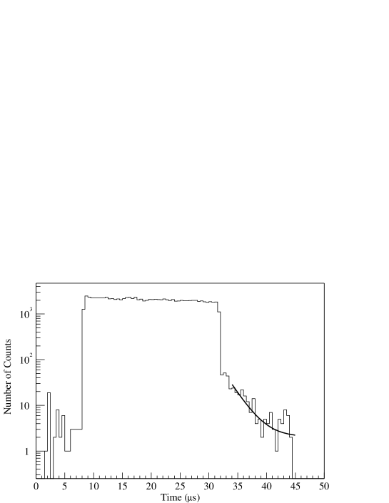
Figure 19: Coincidence event timing spectrum during low-current measurement of the Čerenkov fraction $f_{c}$, showing the period of time after the beam pulse delivery used to estimate the rate of events due to muon decay from $\pi^{+}$ photoproduction. The solid line indicates a fit to the count rate of the form $A+B\,exp[-(t-t_{0})/\tau_{\mu}]$.

The electromagnetic radiative corrections were also computed within the context of the GEANT simulation, using a spin-dependent modification to [119]. In addition to the energy loss that results in a reduction in the four-momentum transferred to the target, electrons emitting radiation prior to interaction with a target nucleus can undergo a spin-flip, effectively depolarizing the incident beam. Such depolarization effects were implemented using the calculations in [120] and [121] for internal and external bremsstrahlung, respectively. Details of the computation of the radiative effects can be found in [122].

In the GEANT simulation, scattered electrons were generated uniformly in energy, angle and along the length of the 40 cm target. Energy loss due to straggling in the aluminum entrance window to the target, and in the thickness of liquid hydrogen upstream of the randomly chosen interaction point, was accounted for before computation of the scattered electron kinematics. Each scattered electron was assigned a cross section and a parity-violating asymmetry, and propagated through the target exit windows and the scattering chamber. A detection efficiency based on the velocity of the outgoing electron and the path length of the event’s track in the Čerenkov medium was combined with the computed cross section as an event weight. Scattered electrons were required to be incident on a mirror and the generated Čerenkov light was required to have a trajectory that, when reflected from a mirror, would be incident on a photomultiplier tube. For the hydrogen target only elastic $e$-$p$ scattering was evaluated. For the deuterium target, the radiative effects were evaluated separately for elastic and inelastic $e$-$d$ scattering, which were then combined, weighted by their relative cross sections.

Table 4 contains a summary of all the dilution corrections for the three experiments, averaged over the ten detectors. A summary of the systematic uncertainties for each of the three measurements is shown in Table 5.

Data set	$f_{l}$	$f_{c}$	$(1-f_{\pi})$	$R_{c}$	$P_{B}$
H2 200 MeV	0.83	0.86	0.96	1.13	36.2%
D2 200 MeV	0.71	0.89	0.90	1.12	35.7%
D2 125 MeV	0.76	0.90	1.00	1.09	38.9%

Table 4: Summary of dilution corrections for the three SAMPLE experiments. The corrections, which varied a small amount for each of the ten detectors, were applied on a detector-by-detector basis. The light fraction $f_{l}$ and Cerenkov fraction $f_{c}$ were determined directly from experimental data as described above, whereas $f_{\pi}$ and $R_{C}$ had to be determined from the GEANT simulation.

Source		$\delta A/A$ (%)
	H2 200 MeV	D2 200 MeV	D2 125 MeV
Beam polarization	4	4	3
Čerenkov fraction	4	3	3
Radiative correction	3	3	3
Pion contamination	2	2
Net dilution factor	7	6	5
Background asymmetry subtraction	13		5
Asymmetry Corrections Procedure	6	5	5
Luminosity Monitor Asymmetry	1	2	14
Total (quadrature sum)	16	9	17

Table 5: Summary of systematic uncertainties for the three data sets, indicated as a relative uncertainty in the measured asymmetry.

2.4 Results from the Hydrogen Data

A preliminary analysis of the hydrogen data was published in [123]. Both the analysis and the theoretical expectation were since refined, as described above: the main modification to the theoretical expectation was to recast the one-body weak radiative corrections using the $\overline{\mathrm{MS}}$ value for $\sin^{2}\theta_{W}$, which resulted in a significant reduction because of their dependence on $(1-4\sin^{2}\theta_{W})$.

Differences between the first analysis and the subsequent one are discussed in detail in [122] and [2], primarily coming from use of the GEANT simulation to compute the radiative corrections and pion dilution correction (as described in section 2.3), as well as the treatment of the shutter CLOSED background. The measured background asymmetry, when averaged over the ten detectors, of $-0.62\pm 0.69$ ppm was consistent with zero but the detector-by-detector distribution was not flat. It had a dependence on the azimuthal angle $\phi$ about the beam axis, and a fit to a function $f(\phi)=A_{0}+A_{1}\cos(2\phi+\phi_{0})$ fit the data with significantly better $\chi^{2}$/d.o.f (8.0/7) than the presumed flat distribution (33.3/9). This $\phi$-dependent behavior is not evident in the shutter OPEN data with any statistical significance. Therefore the OPEN data were combined in a weighted average of the ten detectors, and the fitted value of $A_{0}=-0.06\pm 0.71$ ppm was subtracted from the OPEN asymmetry to yield the result

$$A_{p}(Q^{2}=0.1)=-5.61\pm 0.67\pm 0.88\,{\mathrm{ppm}}\,,$$ (29)

where the first uncertainty is statistical and the second is systematic, including the uncertainty in the background asymmetry. The two distributions as a function of azimuthal angle are shown in Figure 20.

The GEANT simulation was also used to compute the theoretical value to which the data were compared, in order to account for finite acceptance and target length effects in the detector. Because of the integrating nature of the detector system, the simulation was not used to compare directly to the asymmetry data. Dipole form factors were used for the neutron magnetic and proton electromagnetic form factors in computing the $e$-$p$ cross section, and the Galster parameterization for $G_{E}^{n}$. Uncertainties in the predicted asymmetry due to the electromagnetic form factors are small: they are dominated by the uncertainties in $G_{M}^{n}$, for which a 3% uncertainty was assumed, and $G_{M}^{p}$, for which the uncertainty was assumed to be 2%. The resulting effect on $G_{M}^{s}$ is 0.05. The effect of averaging over the target length and acceptance was to reduce the predicted value of the asymmetry by 3%. Other required quantities for computing the asymmetry were $\sin^{2}\theta_{W}=0.23113$, $G_{F}=1.16637\times 10^{-5}$ GeV^-2 [7], ${G_{A}^{e}}^{(T=0)}=-0.07$. The resulting theoretical asymmetry is

$$A_{p}=-5.56+3.37G_{M}^{s}+1.54{G_{A}^{e}}^{(T=1)}$$ (30)

where the asymmetry is in parts per million and the form factor $G_{M}^{s}$ is in nuclear magnetons. Combining the measured hydrogen asymmetry with the theoretically determined value of ${G_{A}^{e}}^{(T=1)}=-0.83\pm 0.26$ results in

$$G_{M}^{s}(Q^{2}=0.1)=0.37\pm 0.20\pm 0.26\pm 0.07$$ (31)

where the last uncertainty is due to knowledge of the electromagnetic form factors and of the electroweak radiative corrections to ${G_{A}^{e}}^{(T=1)}$. The results for individual detector types are listed in Table 6.

Figure 20: Contributions to the asymmetry, corrected for the appropriate dilution factors, from the CLOSED and OPEN shutter data. The CLOSED contribution was best fit to a $\cos 2\phi$ function while for the OPEN data a weighted average of the ten detectors was used.

Det. #	$\langle\theta\rangle$	$A_{0}$	$A_{1}$	$A_{2}$	rel. weight	$A_{meas}$
	(deg)	(ppm)	(ppm)	(ppm)		(ppm)
1,3,8,10	143	-5.49	3.31	1.52	0.48	-5.70$\pm$0.96
2,9	152	-6.11	3.73	1.69	0.19	-4.14$\pm$1.52
4,7	136	-4.90	2.93	1.37	0.24	-4.14$\pm$1.37
5,6	158	-6.53	4.03	1.80	0.09	-12.29$\pm$2.23

Table 6: Summary of experimental results and theoretical expectation for the asymmetry, in ppm, broken down by detector type for the SAMPLE 200 MeV hydrogen data. The quantities $A_{0}$, $A_{1}$ and $A_{2}$ are the leading term and the coefficients multiplying $G_{M}^{s}$ and ${G_{A}^{e}}^{(T=1)}$, respectively. The relative weights were determined by the uncertainty in the measured asymmetries for each detector type. The uncertainty in the experimental result is statistical only: the uncertainty in the background correction was treated as a common systematic error.

2.5 Results from the Deuterium Data

Analysis of the 200 MeV deuterium data, originally presented in [124], has also since been updated [1]. When combined with the result in [123], the data indicated a value of $G_{M}^{s}$ consistent with zero, but a radiative correction to ${G_{A}^{e}}^{(T=1)}$ that was significantly larger than anticipated from theory. A new analysis of both the theoretical expectation and the experimental data were carried out. Three main improvements have led to a new result for ${G_{A}^{e}}^{(T=1)}$ that is now in good agreement with [18]. As described above and in [1], improved determination of the electromagnetic radiative corrections and Čerenkov fractions, as well as accounting for coherent $\pi^{0}$ production, resulted in an increase of the dilution correction by 11%. The measured background asymmetry was consistent with zero and did not exhibit the $\phi$-dependent behavior seen in the hydrogen data. As a result no correction for background asymmetry was applied, resulting in a dilution-corrected asymmetry of

$$A_{d}=-7.77\pm 0.73\pm 0.72\,{\mathrm{ppm}}\,.$$ (32)

In the determination of the theoretical asymmetry to which the result should be compared, again the GEANT simulation was used to identify finite acceptance effects. For the theoretical model, parity-violating and parity-conserving response functions provided by Schiavilla were used that include both quasielastic scattering and threshold breakup of deuterium. The latter process contributes approximately 5% to the experimental yield, with an asymmetry comparable in magnitude to quasielastic scattering. The calculation, based on that described in [125] and [81], used the Desplanques, Donoghue and Holstein [19] parameterization of parity-violating meson exchange coupled with the Argonne V18 $N$-$N$ potential [126]. The anapole contributions were based on [127].

In the computation of the theoretical asymmetry it was also necessary to include a contribution from elastic $e$-$d$ scattering, which is only 1-2% of the detector yield but for which the asymmetry expected to be comparable in magnitude but opposite in sign. It is expected that elastic $e$-$d$ scattering has considerable sensitivity to strange quarks [128]. The elastic asymmetry was evaluated using a global fit to deuteron form factor data [129]. The elastic and inelastic processes were evaluated separately and then combined weighted by the appropriate cross sections. Table 7 contains a summary of the evaluation of the theoretical asymmetry, and the experimental result, broken down by detector type.

The resulting theoretical asymmetry is

$$A_{d}=-7.06+0.72G_{M}^{s}+1.66{G_{A}^{e}}^{(T=1)}\,.$$ (33)

In Figure 21 are shown three bands in the space of $G_{M}^{s}$ vs. ${G_{A}^{e}}^{(T=1)}$ for the hydrogen and deuterium data as well as the prediction of Zhu et al, along with two ellipses representing to 1-$\sigma$ the overlap of the two measurements and also the hydrogen data with the theoretical band. The resulting values of the form factors taken solely from the two data sets are

$$G_{M}^{s} = 0.23\pm 0.36\pm 0.40$$

$${G_{A}^{e}}^{(T=1)} = -0.53\pm 0.57\pm 0.50\,,$$ (34)

in good agreement with [18] and with the determination of $G_{M}^{s}$ from the hydrogen data alone.

Det. #	$\langle\theta\rangle$	$A_{0}$	$A_{1}$	$A_{2}$	rel. weight	$A_{meas}$
1,3,8,10	143	-7.04	0.76	1.65	0.49	-8.37$\pm$1.03
2,9	152	-7.66	0.83	1.77	0.16	-10.13$\pm$1.85
4,7	136	-6.37	0.73	1.55	0.26	-6.21$\pm$1.43
5,6	158	-8.09	0.88	1.85	0.07	-4.99$\pm$2.36

Table 7: Summary of experimental results and theoretical expectation for the asymmetry, in ppm, broken down by detector type for the SAMPLE 200 MeV deuterium data. The quantities $A_{0}$, $A_{1}$ and $A_{2}$ are the leading term and the coefficients multiplying $G_{M}^{s}$ and ${G_{A}^{e}}^{(T=1)}$, respectively. The relative weights were determined by the uncertainty in the measured asymmetries for each detector type.

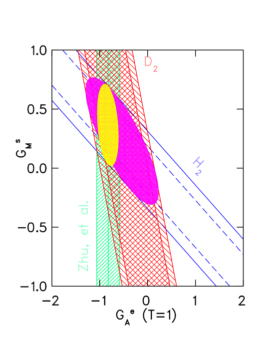
Figure 21: Results from the 200 MeV SAMPLE data, in the space of $G_{M}^{s}$ vs. ${G_{A}^{e}}^{(T=1)}$, along with the theoretically expected value of ${G_{A}^{e}}^{(T=1)}$, using [18] for the weak radiative corrections. The ellipses correspond to a 1-$\sigma$ overlap of the two data sets (larger) and the hydrogen data and theory (smaller).

In order to provide another experimental determination of ${G_{A}^{e}}^{(T=1)}$, a third SAMPLE measurement was carried out at a lower beam energy of 125 MeV, corresponding to a momentum transfer of 0.04 (GeV/c)². The experimental method and apparatus were identical to the 200 MeV measurements, as was the procedure for determining the dilution corrections and the physics asymmetry. Three additional systematic uncertainties were required in order to account for effects seen in this measurement not present in the earlier ones. First, a nonzero helicity correlation in the beam transmission, caused by differential beam scraping and an energy-defining slit in the accelerator, was seen in one of the two half-wave plate states. As a result beam transmission was used as a parameter in the linear regression to remove helicity correlated beam effects. Because this correction was larger in one half-wave plate state than the other (0.14 ppm vs. 0.03 ppm prior to application of dilution corrections), the relative uncertainty in the correction was also correspondingly larger (11.2% vs. 2%). The uncertainty in the corrections procedure was determined by comparing the size of the correction using the dependence of the detector yield on unpolarized beam properties with that using the dependence of the detector asymmetry on beam helicity correlations. Secondly, the forward angle luminosity monitors had a nonzero asymmetry even after the corrections procedure was applied. While in principle the main detector and luminosity monitor signals should be uncorrelated, a nonzero luminosity asymmetry could be indicative of an unaccounted for helicity correlated beam property. The magnitude of potential false asymmetry in the Čerenkov detector was estimated by multiplying the luminosity monitor asymmetry with the correlation between the Čerenkov detector asymmetry and the luminosity monitor asymmetry, resulting in an additional 20% systematic error. Finally, while again the average background asymmetry was consistent with zero, the $\phi$-dependence in the background asymmetry that was present in the 200 MeV hydrogen data (but absent from the 200 MeV deuterium data) was again seen. The asymmetry was measured with dedicated runs by placing a set of scintillators in front of the phototube shutters to enhance the background component, and the background asymmetry was subtracted from the OPEN asymmetry. The systematic uncertainty associated with this procedure was estimated to be 5%. The resulting measured asymmetry was

$$A(Q^{2}=0.038)=-3.51\pm 0.57\pm 0.58\,{\mathrm{ppm}}\,.$$ (35)

The theoretical value to which the measurement should be compared was computed as described above, resulting in

$$A_{d}=-2.14+0.27G_{M}^{s}+0.76{G_{A}^{e}}^{(T=1)}\,{\mathrm{ppm}}\,.$$ (36)

While no corresponding hydrogen data were taken at the lower beam energy, the two deuterium measurements can be compared to theoretically expected values assuming a particular value of $G_{M}^{s}$ at the lower momentum transfer of $Q^{2}=0.038$ (GeV/c)². The dependence of the deuterium asymmetry on $G_{M}^{s}$ is, however, very weak. A comparison between the data and theoretical expectation assuming a constant value of $G_{M}^{s}=0.15$ is shown in Figure 22. The boxes represent the variation in the theory for a change in $G_{M}^{s}$ of 0.6. The good agreement indicates a weak $Q^{2}$ dependence of ${G_{A}^{e}}^{(T=1)}$, consistent with expectation.

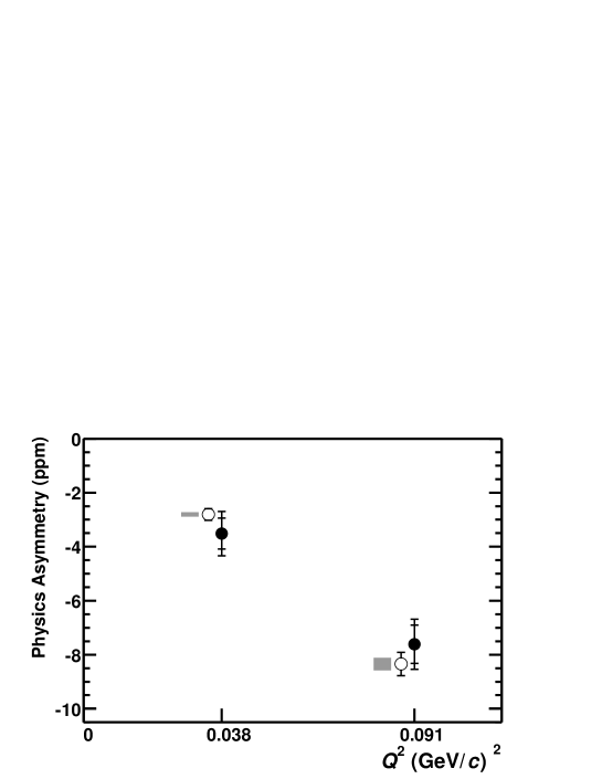
Figure 22: Comparison of the two SAMPLE deuterium measurements (solid circles)  to expectation from theory (open circles) using axial radiative corrections as computed by [18]. The theory also assumes a value of $G_{M}^{s}$ of 0.15 nuclear magnetons. The grey bands represents a change in $G_{M}^{s}$ of 0.6 n.m.

Two additional remarks are in order regarding the SAMPLE experimental measurements. Assuming that a determination of nucleon form factors can ultimately be related to electron quark couplings, the axial form factor measurements in the two deuterium experiments can be recast in terms of the parameters $C_{2u}$ and $C_{2d}$ that represent electron-quark axial couplings. Prior to the SAMPLE measurements the only experimental limits on $C_{2u}$ and $C_{2d}$ were from the first parity-violation electron scattering experiment to be performed [99] and from the parity-violating quasielastic scattering measurement carried out at the Mainz microtron in the mid-1980’s [101]. The two SAMPLE deuterium measurements are sensitive to the combination

$$C_{2u}-C_{2d}=-\frac{{G_{A}^{e}}^{(T=1)}\left(1-4\sin^{2}\theta_{W}\right)}{G_{A}(Q^{2})}\,.$$ (37)

It is modified by the 1-quark radiative corrections, and, in the case of elastic electron-nucleon scattering, it is also modified by the somewhat more uncertain multi-quark corrections discussed in [18]. In order to compare directly to the deep-inelastic scattering data, the multi-quark corrections must be removed from the SAMPLE data. While this is small contribution, it dominates the uncertainty in the radiative corrections. The one-quark radiatively corrected values of the couplings within the context of the Standard Model are $C_{2u}=-0.0360$ and $C_{2d}=0.0265$. Extrapolating the neutral weak axial form factor $G_{A}(Q^{2})$ using the dipole parameterization described in the introduction, and removing the multi-quark corrections results in the following from the SAMPLE deuterium 200 MeV and 125 MeV data sets, respectively.

$$C_{2u}-C_{2d} = -0.042\pm 0.040\pm 0.035\pm 0.02$$

$$C_{2u}-C_{2d} = -0.12\pm 0.05\pm 0.05\pm 0.02\pm 0.01$$ (38)

where third uncertainty is that due to the multi-quark radiative corrections. For the 125 MeV result, the last uncertainty corresponds to variation of $G_{M}^{s}$ by $\pm 0.6$, because it is undetermined at this momentum transfer. These values are in good agreement with the Standard Model prediction, and the improvement over the earlier measurements is shown in Figure 23.

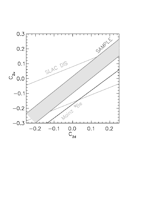
Figure 23: Existing measurements of $C_{2u}$ and $C_{2d}$, shown as 1-$\sigma$ uncertainty bands. Only the 200 MeV SAMPLE result is shown. The prediction for these quantities in the Standard Model, using the global best fit values of the masses of the top quark and Higgs boson and the strong and electromagnetic coupling constants (see  [7]), is $C_{2u}=-0.0360$, $C_{2d}=0.0265$.

Another byproduct of the SAMPLE experiment was the first measurement of the beam spin asymmetry on a nucleon using a transversely polarized beam [130] (also referred to as a vector analyzing power). Scattering from a transversely polarized beam and an unpolarized target produces a parity conserving asymmetry for electrons scattered in opposite directions about the polarization axis. With an azimuthally symmetric detector the asymmetry can be seen as a $\cos\phi$ dependence in the counting rate asymmetry when the beam polarization direction is reversed. It is a time-reversal odd observable that, to lowest order, can only arise from two-photon exchange. Recently there has been renewed interest in two photon processes for two reasons. As discussed above, it has recently been determined that two-photon exchange processes can be an important contribution to the determination of the proton’s electric form factor from unpolarized cross section data. They are also interesting as a probe of nucleon generalized polarizabilities, through virtual Compton Scattering (in which a real photon is emitted).

In each of the SAMPLE measurements, a few days of data taking were spent with the beam polarization aligned transversely, both in and out of plane. The measured asymmetry as a function of azimuthal angle is shown in Figure 24, along with a fit to the data. The $\phi$ dependence in the data can clearly be seen, the amplitude representing the resulting beam spin asymmetry, found to be $A_{T}=-16.4\pm 5.9$ ppm, about a factor of two larger than predicted by the calculation of Afanasev et al. [131], when only ground state protons are considered in the intermediate state between the two photons. Calculations of the beam spin asymmetry were also carried out at higher energies [132], where proton excitations in the intermediate state are expected to be significant, at the kinematics appropriate for the Mainz PVA4 experiment. Two results from the PVA4 experiment have recently been reported [133]: at $E=0.855$ GeV (and $\theta_{e}=35^{\circ}$), $A_{T}=-7.62\pm 2.34\pm 0.80$ ppm and at $E=0.569$ GeV, $-8.28\pm 0.93\pm 0.49$ ppm. The authors of [132] speculate that contributions from threshold meson production, which were neglected in their first calculation, could cause an additional enhancement, and a new calculation that uses the MAID unitary isobar model for the intermediate states has recently become available [134]. Additional measurements of $A_{T}$ at higher momentum transfer are anticipated in the future from the G⁰ and HAPPEX experiments, where simple nucleon excitation in the intermediate state may no longer be an adequate description, but at energies below that appropriate for a parton model description.

Figure 24: Asymmetry as a function of azimuthal angle $\phi$ for transversely polarized beam, as measured in the SAMPLE experiment. The curve is the best fit to a set of four combined measurements.

3 Other Experiments

3.1 HAPPEX at Jefferson Laboratory

The first measurements of parity-violating electron scattering at Jefferson Laboratory [135] were carried out by the HAPPEX collaboration, who used a 3.3 GeV polarized beam on a 15 cm hydrogen target and detected the scattered electrons using the pair of high resolution spectrometers (HRS) in Hall A at 12.5^∘. The measured asymmetry, at $Q^{2}$=0.48 (GeV/c)², is sensitive to the combination $G_{E}^{s}+0.39G_{M}^{s}$. With a counting rate of approximately 1 MHz per spectrometer, the spectrum of scattered electrons was integrated over a 30 ms window. A set of Pb-scintillator total absorption counters was used instead of the standard HRS tracking detector package, but the hardware resolution of the spectrometers was sufficient to spatially separate elastic from inelastic scattering events. Custom electronics with 16-bit analog-to-digital converters and low differential nonlinearity were developed for additional optimization of the detection scheme. The helicity of the beam was flipped at a rate of 30 Hz, with the first of a pair being chosen randomly and the second being chosen as the complement of the first, allowing measurement of the PV asymmetry at a rate of 15 Hz. A half wave plate was either inserted or removed approximately once per day, allowing manual reversal of the beam helicity without changing the electronics. The beam polarization was measured with a combination of a Mott polarimeter near the polarized injector region, a Møller polarimeter on the Hall A beam line, and, for the later running, a Compton polarimeter that operated concurrently with normal data taking. Additional detail and a recent review of the HAPPEX experimental techniques can be found in [136].

The HAPPEX experiment was the first to make use of a strained GaAs photocathode in the polarized electron source for parity violation experiments. The strained cathode allows for the possibility of significantly higher beam polarization, in excess of 70%, but with a quantum efficiency that is lower than normal bulk GaAs by about an order of magnitude. Improvements in laser power over the years, along with the better match between the time distribution of the laser light and the needs for the JLab beam made it possible for HAPPEX to take advantage of the increased polarization. One complication, as discussed above, is that such cathodes usually have an intrinsic analyzing power for linear polarization in the incident laser light that could potentially result in significant helicity correlated position differences of the beam on the experimental target. These effects were kept to a negligible level by insertion of a rotatable half-wave plate in the laser beam and with a feedback system nulling any helicity-correlated intensity asymmetry. This feedback system has continued to improve for the next generation of experiments. New developments in crystal fabrication may eliminate this complication in the future.

The experimentally determined asymmetry from the two HAPPEX runs combined is $A_{exp}=-15.05\pm 0.98\pm 0.56$ ppm, corresponding to $G_{E}^{s}+0.39G_{M}^{s}=0.025\pm 0.020\pm 0.014$ where the last uncertainty is due to knowledge of the nucleon EM form factors. HAPPEX thus precludes most of the parameter space in which $G_{E}^{s}$ and $G_{M}^{s}$ have the same sign at $Q^{2}=0.48$ (GeV/c)², as shown in Figure 25.

The future program for HAPPEX includes a forward angle measurement at $Q^{2}$=0.1 (GeV/c)² on hydrogen [138], as well as the first measurement of the PV asymmetry in elastic electron scattering from helium [139]. Due to the fact that ⁴He is a spin-0, isospin-0, target, only a single weak form factor exists and it can be directly related to $G_{E}^{s}$ with a good model of the ⁴He nucleus. Theoretical expectations are that contributions to the asymmetry from many-body effects in the helium are negligible [140] at low momentum transfer. The combined measurements, or the new hydrogen measurement combined with the SAMPLE result, will result in a determination of the electric strangeness radius $r_{s}^{2}$.

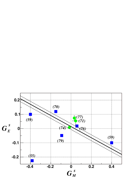
Figure 25: The band shows the allowed region of $G_{M}^{s}$ and $G_{E}^{s}$ at $Q^{2}$=0.48 (GeV/c)² coming from two completed HAPPEX experiments [135], along with several models. The figure is taken with permission from [137], with the reference numbers modified to reflect those in this work. The squares are calculations done prior to the measurement, circles subsequent.

3.2 PVA4 at Mainz

The PVA4 collaboration at Mainz has taken a different experimental approach [141]. The custom detector system has no magnetic field and azimuthal symmetry as in the case of SAMPLE, but is optimized for forward angle measurement. The detector has sufficient segmentation and specialized electronics so that counting the scattered particles is feasible despite very high scattered electron rates. The scattered electrons are detected over a range of angles centered at 35^∘ with a PbF₂ Čerenkov shower calorimeter. The calorimeter design consists of 1022 PbF₂ crystals of 16-20 radiation lengths thickness, arranged in 7 rings, and processed in 3x3 modules with self-triggering and histogramming electronics to collect in real time an energy spectrum of the scattered particles. An energy deposition above a specified threshold triggers the digitization of the summed output of the 3x3 cluster of crystals, in which the charge is integrated over 20 ns and histogrammed. The energy resolution of the detectors must be sufficient to separate the 10 MHz of elastically scattered electrons from the 90 MHz of inelastic electrons coming from threshold pion and resonance production. The achieved energy resolution was 3.5%/$\sqrt{E}$ [142] for 1 GeV particles. A typical energy spectrum of the detected events is shown in Figure 26.

The first PVA4 measurement [143] was at a beam energy of 855 MeV, corresponding to $Q^{2}$=0.23 (GeV/c)² and a sensitivity to the combination $G_{E}^{s}+0.22G_{M}^{s}$, in which half of the detector was instrumented. A 20 $\mu$A beam of polarized electrons was incident on a 10 cm liquid hydrogen target. The beam-target luminosity was monitored with a set of eight water Čerenkov detectors placed symmetrically about the beam line. The beam polarization was approximately 80%, from a strained GaAs in the polarized electron source. The beam helicity was reversed every 20 ms, with an additional manual slow reversal by periodic insertion of an additional half-wave plate. Potential helicity-correlated asymmetries in the incident beam current were kept below several parts per million by adjusting the angle of another, permanently installed, half-wave plate. Beam position and angle incident on the target were measured with microwave cavity monitors, and beam polarization was measured periodically with a Møller polarimeter on a different beam line.

The experimental asymmetry after all dilution corrections was measured to be $A_{exp}=-5.44\pm 0.54\pm 0.26$ ppm [143], with an expectation, assuming no strange quark effects, of $A_{0}=-6.3\pm 0.43$ ppm, where the uncertainty in the theoretical value arises predominantly from uncertainties in the neutron electromagnetic form factors. This difference of approximately 1$\sigma$ hints that $G_{E}^{s}$ and $G_{M}^{s}$ are either both small or have opposite sign. Additional data have already been taken, the run concluding in June 2003, at 570 MeV beam energy, corresponding to $Q^{2}$=0.1 (GeV/c)². Combining these data with the results from SAMPLE will allow the first explicit experimental limits on $G_{E}^{s}$. Future plans involve reversing the orientation of the detector such that scattered electrons can be detected at 140^∘-150^∘ at $Q^{2}$=0.23 and 0.48 (GeV/c)², which, when combined with the existing HAPPEX and PVA4 data would allow separate determination of $G_{E}^{s}$ and $G_{M}^{s}$ over a range of momentum transfer.

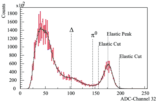
Figure 26: Real-time histogram of the energy spectrum of detected particles in the PbF₂ detector used in the PVA4 experiment at Mainz. The red histogram is the raw data, overlaid with (black line) the spectrum after corrections for differential non-linearity in the analog-to-digital converter.

A summary of the three available measurements of the parity-violating asymmetry in elastic $e$-$p$ scattering is shown in Figure 27, as the deviation of the asymmetry from that expected with no strange quark contributions. While each of the individual measurements is consistent with zero at the 1$\sigma$-level, the three measurements taken together hint at a possible nonzero contribution. The data set is at present insufficient to distinguish between no strange quark contributions and cancellations between $G_{E}^{s}$ and $G_{M}^{s}$. The next generation of experiments, which include the future programs of HAPPEX and PVA4 as well as the G⁰ experiment described below, will address this problem.

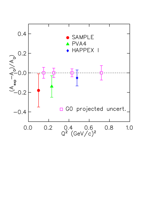
Figure 27: Summary of the available data on parity-violating $e$-$p$ scattering, plotted as the fractional deviation of the measured asymmetry from the expectation with no strange quark contributions. The HAPPEX point is from [137], the PVA4 point from [143], the SAMPLE point from [2], and the G⁰ points are projections of the precision expected from the forward angle running based on information from the 2004 engineering run.

3.3 The G⁰ Experiment at JLab

The G⁰ experiment at JLab is a dedicated apparatus designed to determine $G_{E}^{s}$, $G_{M}^{s}$ and $G_{A}^{e}$ from a single experimental apparatus over a broad $Q^{2}$ range. The detector consists of a superconducting toroidal spectrometer with an array of scintillators along the focal plane to determine the PV asymmetry at both forward and backward scattered electron angles. Polarized electrons are scattered from a 20 cm liquid hydrogen target. In the forward configuration, the recoil protons are detected and sorted by $Q^{2}$ covering the range $0.1<Q^{2}<1.0$ (GeV/c)². A schematic of the apparatus is shown in Figure 28. The flight time from the target to the scintillator array is determined for each scattered particle, allowing the rejection of photoproduced pions and many of the protons generated from inelastic processes. In order to determine the flight times of the detected particles, which range from 5-25 ns, the time structure of the JLab beam is modified from its nominal 2 ns between micropulses to be 32 ns between micropulses. The helicity of the beam is selected pseudo-randomly in a pattern of four “windows”, or quartets, either “$+--+$” or “$-++-$”, such that a new window is selected every 33 ms.  The detected rate approaches 1 MHz, so the flight times are stored electronically and read out as histogrammed data on each helicity reversal. Two complementary sets of electronics are used to read out the detectors: for the odd (North American) octants the arrival time of the events is digitized and then sent to a set of scalers, from which the time-of-flight histogram is reconstructed with a resolution of 1 nsec per time bin. For the even-numbered (French) octants, custom modules were constructed with flash TDCs to digitize and stored the time spectrum, with a resolution of 0.25 nsec per bin, for each 33 ms window. In Figure 29 is shown a typical time spectrum of the scattered events. The inelastically scattered protons that cross under the elastic proton peak are the primary source of background; they come primarily from scattering in the aluminum windows of the target and from pion photoproduction in the liquid hydrogen. The measured asymmetry must be corrected both for any dilution factor and for any potential parity-violating asymmetry associated with these processes. Because this is a counting experiment, the detected rate must also be corrected for electronic deadtime, which has been measured to be 10-15%, and which can produce a false asymmetry if there is a helicity correlated change in the incident beam current. Through a series of tests this correction has been demonstrated to be under control at a level that would produce a negligible false asymmetry in the data. Finally, the data must be corrected for any additional helicity correlations in the position and angle of the incident beam. As discussed in Section 2.1 above, such corrections can be minimized by feedback systems on the laser light that produces the polarized electron beam.

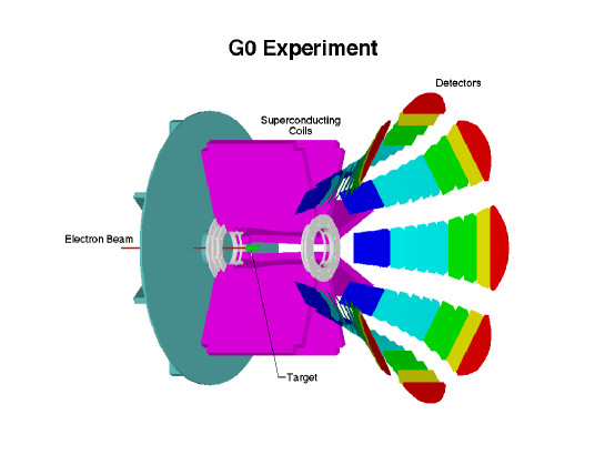
Figure 28: Schematic of the G⁰ apparatus used in its forward-angle configuration. Each detector color corresponds to a different value of momentum transfer $Q^{2}$, ranging from 0.16 (GeV/c)² to 0.9 (GeV/c)².

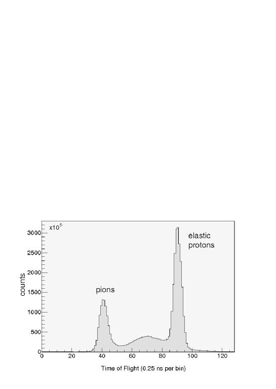
Figure 29: Time of flight histogram, as accumulated in a 33 msec helicity window in the French flash-TDC-based electronics. The left peak is due to photo-produced pions, in the right peak are elastically scattered protons, and the broad distribution in between results from inelastically scattered protons.

The G⁰ collaboration has recently completed its second engineering run and will begin production data taking in mid-March 2004. During this run the asymmetry in the background processes was measured through a combination of empty target and solid target running.

While a definitive determination of the relative signs and/or magnitude of $G_{M}^{s}$ and $G_{E}^{s}$ will require the backward angle measurements as well, this first set of data will both extend the kinematic reach and improve the precision of the data shown in Figure 27.

In order to separately determine $G_{E}^{s}$, $G_{M}^{s}$ and $G_{A}^{e}$, three independent measurements of parity-violating electron scattering are required. The G⁰ experiment will accomplish this by an independent set of measurements with the apparatus reversed such that scattered electrons can be detected in the backward direction at 108^∘. Measurements in this configuration are planned with both hydrogen and deuterium targets to provide the two additional constraints. Three sets of measurements, each requiring a different magnetic field setting, are planned, corresponding to $Q^{2}$ = 0.25, 0.5 and 0.8 (GeV/c)². The scattered electron rate is significantly lower, but is now spread over the entire detector array. Inelastically scattered electrons are discriminated from the elastic electrons of interest with an auxiliary set of detectors at the exit of the magnet cryostat that constrain the tracks of the particles leaving the magnet. The negatively charged pion rate from liquid hydrogen, which can only arise from two-step processes, is low, and thus does not present a significant background, but from liquid deuterium the rate is expected to be appreciable, so a set of aerogel Čerenkov veto counters close to the Cryostat exit detectors will also be added. New custom electronics will identify and sort the elastically scattered events through a coincidence matrix selection. It should be noted that the inelastically scattered electrons, which are primarily due to excitation of the $\Delta$ resonance, will be available for analysis as well [144], thus offering an opportunity to determine the $N$-$\Delta$ axial transition form factor via the weak neutral current process.

4 Future Directions

4.1 Standard Model Tests using Parity-Violating Electron-Nucleon Scattering

The primary focus of this review article is the use of parity-violating electron scattering on the nucleon as a probe of nucleon structure. In the formalism used to extract the strange vector form factors from these experiments, it is assumed that the electroweak Standard Model couplings of the neutral weak $Z$-boson to the quarks summarized in Table 1 are correct. Given the precision with which the strange form factors are anticipated to be determined, this is a reasonable assumption. Historically, the first experimental measurements of parity-violating electron-nucleon scattering of Prescott et al. [99] were measurements of the electroweak quark couplings at a time when the electroweak Standard Model was in its infancy. Since that time, the electroweak Standard Model has been verified to high precision. Its success makes the current set of strange vector form factor measurements possible. With the increased precision now possible in parity-violating electron-nucleon scattering, experiments are being developed to again test the validity of the electroweak Standard Model, thus returning the field to its historical origins. Several new experiments are currently being developed for this purpose.

To motivate the need for new Standard Model tests using parity-violating electron-nucleon scattering, we first briefly review the relevant history in this area. The 1978 experiment of Prescott et al. [99] at SLAC was a measurement of the parity-violating asymmetry in the deep inelastic scattering (DIS) of longitudinally polarized electrons on deuterium. The experiment used incident electron beam energies in the range of 16-22 GeV. This experiment yielded a determination of the weak mixing angle, $\sin^{2}\theta_{W}=0.224\pm 0.020$, which was one of the most accurate determinations at that time. The existence of the neutral weak current had been established earlier in neutrino experiments in 1973, but the extraction of a consistent value of the weak mixing angle from another process was an important confirmation of the validity of the electroweak Standard Model.

In the 1980’s, a large amount of experimental evidence in support of the electroweak Standard Model was accumulated. The most precise measurements of electroweak processes were made in direct production of the $Z$-boson at SLAC’s SLC and CERN’s LEP $e^{+}e^{-}$ colliders. These led to a very accurate and internally self-consistent determination of the weak mixing angle, $\sin^{2}\theta_{W}$, at the $Z$-pole ($Q^{2}=M^{2}_{Z}$). However, relatively few measurements of $\sin^{2}\theta_{W}$ have been made away from the $Z$-pole. Experiments that probe the value of $\sin^{2}\theta_{W}$ far from this value of momentum transfer may reveal physical processes which do not couple strongly to the $Z$ and are outside of the current realm of the Standard Model. As a result, such experiments have an important role in the search for extensions to the Standard Model. Two programs that have been pursued are measurement of parity-violation in atomic systems [145] and of parity-violation in electron-electron (Møller) scattering [146]. In new parity-violating electron-nucleon scattering experiments, precision measurements of $\sin^{2}\theta_{W}$ well below the $Z$-pole ($Q^{2}<<M^{2}_{Z}$) are proposed. To make a meaningful statement, the new generation of parity-violating Standard Model tests anticipate relative uncertainties on $\sin^{2}\theta_{W}$ in the $\sim 0.3-0.7\%$ range, in comparison to the $9\%$ measurement of the original SLAC $e$-$d$ DIS experiment. The advances in polarized electron beam delivery, beam feedback and control, and high power cryotarget technologies appear to make this possible.

4.1.1 The $Q_{weak}$ Experiment at Jefferson Laboratory

The $Q_{weak}$ experiment at Jefferson Laboratory [147] will be a measurement of the proton’s neutral weak charge using parity-violating electron-nucleon scattering. To lowest order in the Standard Model, the proton’s neutral weak charge is the sum of the neutral weak charges of its valence quarks:

$$Q^{p}_{W}=G^{Z,p}_{E}(Q^{2}=0)=2q^{u}_{W}+q^{d}_{W}=1-4\sin^{2}\theta_{W}.$$ (40)

The proposed measurement will yield a precise value of $\sin^{2}\theta_{W}$ at $Q^{2}\sim 0.03\ \hbox{GeV}^{2}$. In the Standard Model, the effective value of $\sin^{2}\theta_{W}$ is predicted to vary with $Q^{2}$, similarly to the running of the coupling constants of QCD and QED. To date, however, the predicted “running of $\sin^{2}\theta_{W}$” in the electroweak Standard Model, shown in Figure 30, has not yet been confirmed experimentally. The predicted shift is $\Delta\sin^{2}\theta_{W}=+0.007$ at low $Q^{2}$ with respect to the $Z$-pole best fit value of $0.23113\pm 0.00015$. Also shown in Figure 30 are data from existing and proposed experiments. Below the $Z$-pole, there are three published data points. The two existing measurements at low $Q^{2}$ are from atomic parity violation experiments in the cesium atom [145], and from a parity-violating Møller scattering experiment at SLAC [146] (E158). The E158 collaboration expects a reduction in their error bar of about a factor of 2 with further data taking. Finally, the NuTeV point is from $\nu$-nucleus deep inelastic scattering [86]. Of the three points, only the NuTeV result appears to show a deviation from the Standard Model. While this could be a signal for new physics, there are more conventional explanations that have been advanced to explain this discrepancy including nuclear effects in the iron target [148], QCD effects [149], and the possibility of non-identical strange sea ($s(x)$ and $\overline{s}(x)$) parton distributions as discussed in Section 1.4. The anticipated relative uncertainty in $\sin^{2}\theta_{W}$ from the $Q_{weak}$ experiment is $\sim 0.3\%$, which would correspond to a 10$\sigma$ deviation from the $Z$-pole value if the running of the weak mixing angle to low $Q^{2}$ is in agreement with the Standard Model prediction. Physics beyond the Standard Model that could enter into $Q^{p}_{W}$ has been considered in [150], which includes extra neutral weak bosons, supersymmetry, and leptoquarks.

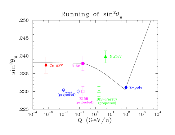
Figure 30: The calculated running of the weak mixing angle in the Standard Model, defined in the modified minimal subtraction scheme [150], is shown as the solid line. The solid data points are from published results: atomic parity violation(APV) [145], parity-violating Møller scattering (E158) [146], deep inelastic neutrino-nucleus scattering (NuTeV) [86], and the world average of $Z$-pole measurements at LEP and SLC. The open symbols are arbitrarily placed on the vertical axis, and they represent proposed experiments: $Q_{weak}$ [147], the anticipated reduction in the E158 error bar after further data taking, and the DIS parity experiments described in section 4.1.2.

The $Q_{weak}$ experiment will provide a measurement of the asymmetry in the elastic scattering of 1.165 GeV longitudinally polarized electrons from an unpolarized liquid hydrogen target. In the limit of forward angle scattering, the asymmetry can be written as:

$$A\sim\left[\frac{-G_{F}}{4\pi\alpha\sqrt{2}}\right][Q^{2}Q^{p}_{W}+Q^{4}B(Q^{2})],$$ (41)

where $Q^{p}_{W}$ is the proton’s weak charge and $B(Q^{2})$ is a hadronic form factor contribution that involves the proton and neutron electromagnetic and neutral weak form factors. The expected data on neutral weak form factors from the forward angle experiments at higher $Q^{2}$ discussed in section 3 is expected to be sufficient to constrain $B(Q^{2})$ so that the uncertainty resulting from this term in the extraction of $Q^{p}_{W}$ will be less than the expected statistical error. At the proposed $Q^{2}=0.03\ \hbox{GeV}^{2}$, the expected asymmetry is $A\sim-0.3\ \hbox{ppm}$. A determination of $\sin^{2}\theta_{W}$ at the desired level of 0.3% requires a determination of $Q^{p}_{W}$ to an accuracy of $\sim 4\%$ (combined statistical and systematic uncertainties).

A conceptual diagram of the $Q_{weak}$ experimental apparatus is shown in Figure 31. The incident $\sim 80\%$ polarized, 180 $\mu$A electron beam will scatter from a 35 cm liquid hydrogen target. Scattered electrons in the range $8\pm 2^{\circ}$ are selected by a precision collimator. A room temperature toroidal magnetic spectrometer focuses elastically scattered electrons onto a focal plane, while inelastic electrons are swept into shielding. The elastically scattered electrons will be detected in 8 quartz Čerenkov bars. Due to the high count rates ($\sim 0.65$ GHz/detector), these detectors will be integrated over a 33 msec window rather than counting individual events. A luminosity monitor located at a very forward angle will be used to monitor for the possible presence of target density fluctuations and to serve as a sensitive detector for any false asymmetries. An auxiliary tracking system consisting of three sets of tracking chambers will be employed at low beam currents to accurately measure the average $\langle Q^{2}\rangle$ of the experiment. High precision electron beam polarimetry will be carried out with the existing Jefferson Lab Hall C Møller polarimeter [151] and a new Compton polarimeter under construction. Further details about the $Q_{weak}$ experiment can be found in [152] and references therein.

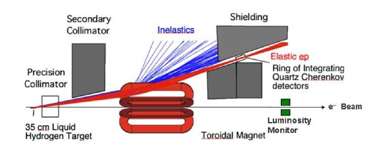
Figure 31: Conceptual diagram of the $Q_{weak}$ experimental apparatus showing the target, collimation system, toroidal magnet, shielding, detectors, and luminosity monitor. The elastically scattered electrons of interest are focused onto the quartz detectors, while the inelastically scattered electrons are swept away.

The observables of low energy parity-violating electron-nucleon scattering experiments can be analyzed in a model-independent way by using the low energy effective neutral current electron-quark Lagrangian given by [7]:

$${\mathcal{L}}^{e-N}=\frac{G_{F}}{\sqrt{2}}\sum_{q}[C_{1q}{\bar{e}}\gamma_{\mu}\gamma^{5}e{\bar{q}}\gamma^{\mu}q+C_{2q}{\bar{e}}\gamma_{\mu}e{\bar{q}}\gamma^{\mu}\gamma^{5}q],$$ (42)

where $C_{1q}$ are the vector quark couplings and $C_{2q}$ are the axial-vector quark couplings. The $Q_{weak}$ experiment will set significant new constraints on $C_{1u}$ and $C_{1d}$ as shown in Figure 32. The shown reduction in the size of the allowed ellipse would result from the precision of the $Q_{weak}$ measurement and its complementarity to existing data. To indicate the ability of low energy experiments to probe new physics possibilities at high energy scales, we consider the case of the vector couplings and define the following [153]:

$${\mathcal{L}}^{PV}_{NEW}=\frac{g^{2}}{4\Lambda^{2}}{\bar{e}}\gamma_{\mu}\gamma_{5}e\sum_{q}h_{V}^{q}\ {\bar{q}}\gamma^{\mu}q,$$ (43)

as a particular parameterization of new physics. Here, $g$, $\Lambda$, and $h_{V}^{q}$ are, respectively, the coupling constant, the mass scale, and effective coefficients that are used to parameterize possible new physics beyond the Standard Model. In the case of $Q_{weak}$, a 4% measurement of $Q_{W}^{p}$ would test new physics scales up to

$$\frac{\Lambda}{g}\sim\frac{1}{\sqrt{\sqrt{2}G_{F}|\Delta Q_{W}^{p}|}}\approx 4.6~{}\hbox{TeV}.$$ (44)

Thus, precision low energy experiments with virtual exchange probes are sensitive to new physics at energies comparable to the scales where colliders can produce the new physics-related particles directly.

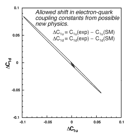
Figure 32: Present and anticipated 90% confidence level constraints on the possibility of deviations of the electron-quark vector couplings from the Standard Model values. The larger ellipse denotes the present limits derived from atomic parity violation [145], parity-violating elastic scattering from the ¹²C nucleus [100], and the SLAC DIS $e-d$ experiment [99]. The smaller, shaded ellipse shows the constraints after the inclusion of a measurement with the expected $Q_{weak}$ precision; the ellipse is centered on the Standard Model prediction.

4.1.2 Parity Violation in Deep Inelastic Scattering

The original experiment of Prescott et al. [99] utilized parity-violating deeply inelastic (DIS) electron scattering from deuterium. Recently, there have been several proposals to measure this process with higher precision. One proposed experiment would use 36 and 39 GeV polarized electron beams at SLAC [154]. Experiments have also be proposed at Jefferson Lab with 6 GeV [155] and with the future upgraded energy of 12 GeV [156].

The parity-violating asymmetry for scattering longitudinally polarized electrons from partons in an unpolarized deuterium target is given by [158]:

$$A_{d}=\frac{\sigma_{R}-\sigma_{L}}{\sigma_{R}+\sigma_{L}}=\left(\frac{3G_{F}Q^{2}}{\pi\alpha 2\sqrt{2}}\right)\frac{2C_{1u}-C_{1d}[1+R_{s}(x)]+Y(2C_{2u}-C_{2d})R_{v}(x)}{5+R_{s}(x)},$$ (45)

where $C_{1u},C_{1d},C_{2u},\ \hbox{and}\ C_{2d}$ are the model independent electron quark couplings defined in Equation 42. The ratios $R_{s}(x)$ and $R_{v}(x)$ are ratios of quark distribution functions. The quantity $Y$ is a function of the kinematic variable $y=\nu/E$, where $\nu=E-E^{\prime}$ is the energy lost by an incident electron of energy $E$ scattering to an electron of energy $E^{\prime}$. A simplified expression for the asymmetry, appropriate to the kinematics of the proposed measurements, is:

$$A_{d}\sim-10^{-4}Q^{2}[(2C_{1u}-C_{1d})+Y(2C_{2u}-C_{2d})]$$ (46)

The dependence of this expression on $Y$ allows for separate extraction of the vector ($2C_{1u}-C_{1d}$) and axial-vector ($2C_{2u}-C_{2d}$) combinations. For typical kinematics of the proposed experiments, $A\sim 100\ \hbox{ppm}$, which is a large asymmetry compared to the current generation of experiments. The experiments can be interpreted in terms of the Standard Model by using the Standard Model values of the weak charges from Table 1:

$$C_{1u} = g^{e}_{A}g^{u}_{V}=-\frac{1}{2}+\frac{4}{3}\sin^{2}\theta_{W}$$

$$C_{1d} = g^{e}_{A}g^{d}_{V}=\frac{1}{2}-\frac{2}{3}\sin^{2}\theta_{W}$$

$$C_{2u} = g^{e}_{V}g^{u}_{A}=-\frac{1}{2}+2\sin^{2}\theta_{W}$$

$$C_{2d} = g^{e}_{V}g^{d}_{A}=\frac{1}{2}-2\sin^{2}\theta_{W}.$$

The currently proposed DIS-parity experiments aim to provide precision measurements of $\sin^{2}\theta_{W}$ in the range $Q^{2}\sim 2-20\ \hbox{GeV}^{2}$. As seen in Figure 30, this is the same $Q^{2}$ range in which the NuTeV collaboration reports a deviation from the Standard Model expectation. As pointed out in section 4.1.1, the NuTeV experiment could potentially be explained by more conventional mechanisms. The DIS-parity experiments on deuterium would be an important cross-check on this result, because they would not be impacted by the same uncertainties in nuclear effects and nuclear parton distributions that are present in the NuTeV measurement on an iron target. When analyzed in the model independent framework described in section 4.1.1, the primary impact of the DIS-parity experiments described here will be to reduce the allowed phase space of the axial coupling combination, $2C_{2u}-C_{2d}$ . The current limits on these couplings are shown in Figure 23. Possible new physics extensions to the Standard Model that would be present in DIS-parity experiments have been considered in Kurylov, et al. [157].

The proposed DIS-parity experiment at SLAC [154] would scatter 36 and 39 GeV polarized electron beams from a 100 cm liquid deuterium target. Scattered electrons would be detected in two large solid angle magnetic spectrometers at a mean scattering angle of $\sim 12^{\circ}$. The electrons would be identified and counted in an array of Pb-glass blocks, with a gas Čerenkov counter to aid in particle identification. The experiment will be run at two different beam energies because the electron spin precesses by $\pi$ between the two beam energies due to its anomalous moment. The resulting change in sign of the measured asymmetry is a useful systematic check for false asymmetries. This anticipated result of this experiment would be a 0.4% (combined relative error) determination of $\sin^{2}\theta_{W}$ at $Q^{2}=20\ \hbox{GeV}^{2}$.

At Jefferson Lab, there are ideas to do DIS-parity at both 6 GeV and eventually the upgraded 12 GeV beam energy. The proposal at 6 GeV [155] would use a 140 $\mu$A, 6 GeV, 80% polarized electron beam incident on a 15 cm liquid deuterium target. The scattered electrons will be detected in the two Hall A High Resolution Spectrometers (HRS) at a scattering angle of $19^{\circ}$. The expected asymmetry in this kinematics is about 131 ppm and the anticipated result would be a 1.0% (combined relative error) determination of $\sin^{2}\theta_{W}$ at $Q^{2}=2\ \hbox{GeV}^{2}$. With an upgraded CEBAF accelerator energy of 12 GeV, a possible 11 GeV DIS-parity experiment have been evaluated [156]. An experiment with 90 $\mu$A of 80% polarized electron beam incident on a 60 cm liquid deuterium target with upgraded Hall A or Hall C spectrometers could give a 0.6% (combined relative error) determination of $\sin^{2}\theta_{W}$ at $Q^{2}=3\ \hbox{GeV}^{2}$. One potential concern with the Jefferson Lab measurements is the presence of higher twist QCD contributions at the relatively low momentum transfer involved. The expression for the asymmetry in Equation 45 only includes twist-two (”free-parton”) contributions. The formalism for including higher twist (quark-gluon correlation) contributions is described in  [159]. If higher twist effects turn out to be significant, then measurements at several values of $Q^{2}$ and $x$ will be necessary to separate the higher twist effects from the weak mixing angle determination.

4.2 Summary

Since the earliest measurements of Prescott and collaborators [99], basic techniques of parity-violating electron scattering have remained more or less the same. But the achievable precision has greatly improved as a result of new high intensity electron beams, advances in polarized beam technology, and technical advances in the feedback and laser systems that are needed for polarized beam delivery. In the last decade, the focus of new experiments has been to use the neutral weak interaction as a probe of hadron structure in a way that is complementary to the large body of information from electromagnetic probes. Although the experiments remain challenging, results from the first round of experiments are now available. While these data have provided an initial look at the role of strange quarks in the proton’s electromagnetic properties, ambiguities remain because these experiments cannot yet distinguish between small values of $G_{M}^{s}$ and $G_{E}^{s}$ or cancellations due to differing signs. In the next few years, new results will be available from HAPPEX, PVA4 and from the G0 Experiment at Jefferson Lab, all of which should help answer this question. The precision with which this generation of experiments will constrain these hadronic structure issues will be sufficient to allow for a future program of parity-violating electron-nucleon scattering that is again focused on a determination $\sin^{2}\theta_{W}$.

The authors gratefully acknowledge financial support from the National Science Foundation. We also wish to acknowledge all members of the SAMPLE collaboration, who are listed in Refs. [1] and [2]. Much of the work discussed in this paper has been supported both by the NSF and the U.S. Dept. of Energy.

References

- [1] T. Ito et al., Phys. Rev. Lett. 92, 102003 (2004).
- [2] D.T. Spayde, et al., Phys. Lett. B 58, 79 (2004).
- [3] K.S. Kumar and P.A. Souder, Prog. Part. Nucl. Phys. 45, S333 (2000).
- [4] D.H. Beck and B.R. Holstein, Int. J. Mod. Phys. E10, 1 (2001).
- [5] D.H. Beck and R.D. McKeown, Ann. Rev. Nucl. Part. Sci. 51,189 (2001).
- [6] M.J. Musolf, T.W. Donnelly, J. Dubach, S.J. Pollock, S. Kowalski, and E.J. Beise, Physics Reports 239, 1 (1994).
- [7] Review of Particle Properties, K. Hagiwara et al., Phys. Rev. D66, 010001 (2002).
- [8] A. Liesenfeld et al., Phys. Lett. B 468, 20 (1999).
- [9] V. Bernard, L. Elouadrhiri and U.-G. Meissner, J. Phys. G 28, R1 (2002).
- [10] H. Budd, A. Bodek, and J. Arrington, arXiv:hep-ex/0308005.
- [11] D.B. Kaplan and A. Manohar, Nucl. Phys. B310, 527 (1988).
- [12] R. McKeown, Phys. Lett. B219, 140 (1989).
- [13] D.H. Beck, Phys. Rev. D39, 3248 (1989).
- [14] V. Dmitrasinovic and S.J. Pollock, Phys. Rev. C52, 1061 (1995).
- [15] G. Miller, Phys. Rev. C57, 1492 (1998).
- [16] R. Lewis and N. Mobed, Phys. Rev. D59, 073002 (1999).
- [17] M.J. Musolf and B.R. Holstein, Phys. Lett. B 242, 461 (1990).
- [18] S.-L. Zhu, S.J. Puglia, B.R. Holstein, and M.J. Ramsey-Musolf, Phys. Rev. D 62, 033008 (2000).
- [19] B. Desplanques, J.F. Donoghue and B.R. Holstein, Ann. Phys. (NY) 124, 449 (1980).
- [20] See, for example, “Quarks and Leptons” by F. Halzen and A.D. Martin, John Wiley and Sons, Inc., 1984.
- [21] A.I. Akhiezer and M.P. Rekalo, Sov. Phys.-Diklady 13, 572 (1968).
- [22] N. Dombey, Rev. Mod. Phys. 41, 236 (1969).
- [23] A.I. Akhiezer and M.P. Rekalo, Sov. J. Part. Nucl. 3, 277 (1974).
- [24] R. Arnold, C. Carlson, and F. Gross, Phys. Rev. C23, 363 (1981).
- [25] M. K. Jones, et al., Phys. Rev. Lett. 84, 1398 (2000).
- [26] O. Gayou, et al., Phys. Rev. Lett. 88, 092301 (2002).
- [27] V. Punjabi et al., submitted to Phys. Rev. C, 2003.
- [28] J.R. Arrington, Phys. Rev. C 68, 034325 (2003). See also ibid, Phys. Rev. C 69, 032201 (2003).
- [29] M.E. Christy, et al., arXiV:nucl-ex/0401030.
- [30] P.A.M. Guichon and M. Vanderhaeghen, Phys. Rev. Lett. 91, 142303 (2003).
- [31] P.G. Blunden, W. Melnitchouk, J.A. Tjon, Phys. Rev. Lett.91, 142304 (2003).
- [32] J.R. Arrington, Phys. Rev. C 69, 022201 (2004).
- [33] Jefferson Laboratory experiment E01–001, J. Arrington and R. Segal, contacts.
- [34] Jefferson Laboratory experiment E01–109, C. Perdrisat, contact.
- [35] JLab proposals (contacts): PR–04–008 (X. Jiang), PR–04–009 (D. Mack), E–04–019 (R. Suleiman), PR–04–020 (J.R. Arrington), and S.P. Wells (G0–experiment), private communication.
- [36] H. Gao, Int’l. Jour. Mod. Phys. E12, 1 (2003) and ibid., p. 567 (arXiv:nucl-ex/0310002).
- [37] R. Alarcon, et al., BLAST collaboration (2003) (http://blast.lns.mit.edu).
- [38] W. Xu, et al., Phys. Rev. Lett. 85, 2900 (2000).
- [39] W. Xu, et al., Phys. Rev. C67, R012201 (2003).
- [40] G. Kubon et al., Phys. Lett.B 524, 26 (2002).
- [41] E.E.W. Bruins, et al., Phys. Rev. Lett. 75, 21 (1995).
- [42] H. Anklin, et al., Phys. Lett. B 428, 248 (1998).
- [43] Jefferson Laboratory experiment E94–017, W. Brooks, contact.
- [44] R. Schiavilla and I. Sick, Phys. Rev. C64, 041002 (2001).
- [45] D. Abbott, et al., Euro. Phys. Jour. A 7, 421 (2000).
- [46] R. Madey, et al., Phys. Rev. Lett. 91, 122002 (2003).
- [47] G. Warren, et al., Phys. Rev. Lett. 92, 042301 (2004).
- [48] M. Ostrick, et al., Phys. Rev. Lett. 83, 276 (1999).
- [49] J. Bermuth, et al., Phys. Lett. B 564, 199 (2003).
- [50] R.L. Jaffe, Phys. Lett. B 229, 275 (1989).
- [51] G. Höhler, Nucl. Phys. B 224, 505 (1976).
- [52] H. Forkel, Phys. Rev. C 56, 510 (1997).
- [53] P. Mergell, U.-G. Meissner, and D. Drechsel, Nucl. Phys. A596, 367 (1996).
- [54] H.-W. Hammer, U.-G. Meissner, and D. Drechsel, Phys. Lett. B 367, 323 (1996).
- [55] M.J. Musolf, H.-W. Hammer, and D. Drechsel, Phys. Rev. D55, 2741 (1997).
- [56] M.J. Ramsey-Musolf and H.-W. Hammer, Phys. Rev. Lett. 80, 2539 (1998).
- [57] H.-W. Hammer and M.J. Ramsey-Musolf, Phys. Rev. C60, 045205 (1999).
- [58] H.-W. Hammer and M.J. Ramsey-Musolf, Phys. Rev. C60, 045204 (1999).
- [59] L. Hannelius, D.O. Riska and L. Ya. Glozman, Nucl. Phys. A 665, 353 (2000).
- [60] W. Koepf, E.M. Henley, and S.J. Pollock, Phys. Lett. B 228, 11 (1992).
- [61] M.J. Musolf and M. Burkardt, Z. Phys. C61, 433 (1994).
- [62] P. Geiger and N. Isgur, Phys. Rev. C55, 299 (1997).
- [63] T.R. Hemmert, U-G. Meissner, and S. Steininger, Phys. Lett. B437, 184 (1998).
- [64] M.J. Ramsey-Musolf and H. Ito, Phys. Rev. C 55, 3066 (1997).
- [65] B.A. Mueller, et al., Phys. Rev. Lett. 78, 3824 (1997).
- [66] K. Aniol, et al., Phys. Rev. Lett. 82, 1096 (1999).
- [67] H.-W. Hammer, S.J. Puglia, M.J. Ramsey-Musolf, and S.-L. Zhu, Phys. Lett. B 562, 208 (2003).
- [68] S.J. Dong, K.F. Liu, and A.G. Williams, Phys. Rev. D 58, 074504 (1998).
- [69] R. Lewis, W. Wilcox, and R.M. Woloshyn, Phys. Rev. D 67, 013003 (2003).
- [70] D. Leinweber and A.W. Thomas, Phys. Rev. D 62, 074505 (2000).
- [71] L. Hannelius and D.O. Riska, Phys. Rev. C 62, 045204 (2000).
- [72] V.E. Lyubovitskij, P. Wang, Th. Gutsche, and A. Faessler, Phys. Rev. C 66, 055204 (2002).
- [73] H.-C. Kim, T. Watabe and K. Goeke, Nucl. Phys. A 616, 606 (1997). See also, A. Silva, H.-C. Kim and K. Goeke, Phys. Rev. D 65, 014016 (2001) and A. Silva, H.-C. Kim and K. Goeke, arXiv:hep-ph/0210189.
- [74] H. Weigel, A. Abada, R. Alkofer and H. Reinhardt, Phys. Lett. B 353, 20 (1995).
- [75] A. Silva, H.-C. Kim and K. Goeke, Phys. Rev. D 65, 014016 (2002), erratum-ibid. D 66, 039902 (2002).
- [76] N.W. Park and H. Weigel, Phys. Lett. B 268, 155 (1991).
- [77] N.W. Park and H. Weigel, Nucl. Phys. A 541, 453 (1992).
- [78] E. Hadjimichael, G.I. Poulis, and T.W. Donnelly, Phys. Rev. C 45, 2666 (1992).
- [79] L. Diaconescu, R. Schiavilla, and U. van Kolck, Phys. Rev. C 63, 044007 (2001).
- [80] C.P. Liu, G. Prezeau, and M.J. Ramsey-Musolf, Phys. Rev. C 67, 035501 (2003).
- [81] R. Schiavilla, J. Carlson, and M. Paris, Phys. Rev. C 67, 032501 (2003).
- [82] W.-Y.P. Hwang, E.M. Henley, and G.A. Miller, Ann. Phys. (N.Y.) 129, 47 (1981).
- [83] Los Alamos npdgamma experiment, D. Bowman, spokesperson.
- [84] M. Goncharov, et al., Phys. Rev. D 64, 112006 (2001).
- [85] H.L. Lai, et al. Phys. Rev. D 55, 1280 (1997).
- [86] G.P. Zeller, et al., Phys. Rev. Lett. 88, 091802 (2002).
- [87] “A Combination of Preliminary Electroweak Measurements and Constraints on the Standard Model”, CERN-EP/2001-98, hep-ex/0112021.
- [88] T.P. Cheng and R. Dashen, Phys. Rev. Lett. 26, 594 (1971).
- [89] M.G. Olsson, Phys. Lett. B 482, 50 (2000).
- [90] See, e.g., M.E. Sainio, Proceedings of the 7th International Symposium on Meson-Nucleon Physics and the Structure of the Nucleon, (Universitaä t Karlsruhe, UCLA, 1997), eds. D. Drechsel et al., pp. 144-149, and references therein.
- [91] M.M Pavan and R.A. Arndt, PiN Newslett. 15 (1999) 118-122
- [92] J. Gasser, H. Leutwyler, and M.E. Sainio, Phys. Lett. B 253, 252 (1991).
- [93] S. Wright, D. Leinweber, and A.W. Thomas, Nucl. Phys. A680, 137c (2001).
- [94] B.W. Filippone and X. Ji, Adv. Nucl. Phys. 26,1 (2001).
- [95] A. Airepetian, et al., Phys. Rev. Lett 92, 012005 (2004).
- [96] L.A. Ahrens et al., Phys. Rev. D 35, 785 (1987).
- [97] G.T. Garvey, W.C. Louis, and D.H. White, Phys. Rev. C 48, 761 (1993).
- [98] S. Pate, Phys. Rev. Lett. 92, 082002 (2004).
- [99] C.Y. Prescott et al., Phys. Lett. B 84, 524 (1979).
- [100] P.A. Souder et al., Phys. Rev. Lett. 65 (1990).
- [101] W. Heil et al., Nucl. Phys. B 327, 1 (1989).
- [102] M. Farkhondeh et al., Proceedings of the Fifteenth International Conference on Applications of Accelerators in Research and Industry, AIP Conf. Proc. CP475, 261 (1999).
- [103] L.B. Levchuk, Nucl. Inst. Meth. A345, 496 (1994).
- [104] J. Arrington et al., Proceedings of the 12th International Symposium on High Energy Spin Physics, World Scientific, 813 (1997).
- [105] D.H. Barkhuff et al., Nucl. Inst. Meth. A450, 187 (2000).
- [106] Z.D. Farkas et al., Recent Developments in Microwave Beam-Position Monitors at SLAC, SLAC Preprint SLAC-PUB-1823 (1976).
- [107] T. Averett et al., Nucl. Inst. Meth. A438, 246 (1999).
- [108] E. Beise et al., Nucl. Inst. Meth. A 378, 383 (1996).
- [109] R. Hasty, Ph.D. thesis, Univ. Illinois, 2003, unpublished.
- [110] S.-P. Li, E.M. Henley, and W.-Y.P. Hwang, Ann. Phys. 143, 372 (1982).
- [111] H.-W. Hammer and D. Drechsel, Zeit. Phys. A 353, 321 (1995).
- [112] J.-W. Chen and X. Ji, Phys. Lett.B 501, 209 (2001).
- [113] J.-W. Chen and X. Ji, Phys. Rev. Lett. 86, 4239 (2001).
- [114] GEANT, CERN Program Library.
- [115] H.W. Baer, K.M. Crowe, and P. Truol, “Advances in Nuclear Physics”, vol. 9 (1977).
- [116] J.C. Bergstrom et al., Phys. Rev. C 57, 3203 (1998).
- [117] J.C. Bergstrom, Phys. Rev. C 58, 2574 (1998).
- [118] See, for example, S.R. Beane et al., Nucl. Phys. A 618, 381 (1997).
- [119] L.W. Mo and Y.S. Tsai, Rev. Mod. Phys. 41,205 (1969). See also, Y.S. Tsai, SLAC-PUB-848, 1971.
- [120] T.V. Kuchto and N.M. Shumeiko, Nucl. Phys. B 219, 412 (1983).
- [121] H. Olsen and L.C. Maximon, Phys. Rev. 114, 887 (1959).
- [122] D.T. Spayde, Ph.D. thesis, Univ. Maryland, 2001, unpublished, available at http://www.physics.umd.edu/enp/theses/
- [123] D.T. Spayde et al., Phys. Rev. Lett. 84, 1106 (2000).
- [124] R. Hasty et al., Science 290, 2117 (2000).
- [125] J. Carlson, R. Schiavilla, V.R. Brown and B.F. Gibson, Phys. Rev. C 65, 035502 (2002).
- [126] R.B. Wiringa, V.G.J. Stoks, and R. Schiavilla, Phys. Rev. C 51, 38 (1995).
- [127] W. Haxton, E.M.Henley, and M.J. Musolf, Phys. Rev. Lett. 63, 949 (1989).
- [128] S.J. Pollock, Phys. Rev. D 42, 3010 (1990).
- [129] D. Abbott at al., Euro. Phys. Jour. A 7, 421 (2000).
- [130] S.P. Wells, et al., Phys. Rev. C 63, 064001 (2001). Note that the numerical value of the asymmetry has been updated using the final dilution factors, and are to be published in an erratum.
- [131] A. Afanasev, I. Akushevich, and N.P. Merenkov, hep-ph/0208260.
- [132] M. Vanderhaeghen, private communication.
- [133] S. Baunack, presented at the PAVI04 workshop on parity violation in electron scattering, to appear in the proceedings.
- [134] B. Pasquini and M. Vanderhaeghen, arXiv:hep-ph/0405303.
- [135] K. Aniol, et al., Phys. Lett B 509, 211 (2001). See also K. Aniol, et al., Phys. Rev. Lett. 82, 1096 (1999).
- [136] K. Kumar and P.A. Souder, Prog. Part. Nucl. Phys. 45, S333 (2000).
- [137] K. Aniol, et al., arXiV:nucl-ex/0402004, submitted to Phys. Rev. C (D. Armstrong, private communication).
- [138] JLAB experiment E99–115, K. Kumar and D. Lhuillier, contacts.
- [139] JLab experiment E00–114, D. Armstrong and R. Michaels, contacts.
- [140] M.J. Musolf and T.W. Donnelly, Phys. Lett. B 318, 263 (1993).
- [141] Mainz experiment “PVA4”, D. von Harrach, spokesman.
- [142] J. van de Wiele and M. Morlet, for the A4 collaboration, Czech. Jour. Phys. 53, A1 (2003). An updated experimental result was provided for this conference by F. Maas, private communication.
- [143] F. Maas, et al., submitted to Phys. Rev. Lett., arXiV:nucl-ex/0401019.
- [144] JLab experiment E01–115, S.P. Wells, contact.
- [145] S.C. Bennett and C.E. Wieman, Phys. Rev. Lett. 82, 2484 (1999).
- [146] P.L. Anthony, et al., hep-ex/0312035.
- [147] JLAB experiment E02-020, R. Carlini, contact person.
- [148] G.A. Miller and A.W. Thomas, hep-ex/0204007.
- [149] S. Davidson, et al., J. High Energy Phys. 02, 037 (2002).
- [150] J. Erler, A. Kurylov, and M.J. Ramsey-Musolf, Phys. Rev. D 68, 016006 (2003).
- [151] M. Hauger, Nucl. Inst. Meth. A461, 382 (2001).
- [152] G. Mitchell, et al., hep-ex/0308049.
- [153] M. J. Ramsey-Musolf, Phys. Rev. D 62, 056009 (2000).
- [154] J.R. Arrington, et al., Letter of Intent to SLAC, (2003).
- [155] JLAB Letter of Intent LOI-03-106, X.Zheng, contact person.
- [156] Pre-Conceptual Design Report for The Science and Experimental Equipment for The 12 GeV Upgrade of CEBAF (2003) (http://www.jlab.org/div_dept/physics_division/pCDR_public/pCDR_12-1/)
- [157] A. Kurylov, M.J. Ramsey-Musolf, and S. Su, Phys. Lett. B 582, 222 (2004).
- [158] R. Cahn and F. Gilman, et al., Phys. Rev. D 17, 1313 (1978).
- [159] P. Castorina and P.J. Mulders, Phys. Rev. D31, 2760 (1985).