Method of Monte Carlo grid for data analysis

Abstract

This paper presents an analysis procedure for experimental data using theoretical functions generated by Monte Carlo. Applying the classical chi-square fitting procedure for some multiparameter systems is extremely difficult due to a lack of an analytical expression for the theoretical functions describing the system. The proposed algorithm is based on the least square method using a grid of Monte Carlo generated functions each corresponding to definite values of the minimization parameters. It is used for the E742 experiment (TRIUMF, Vancouver, Canada) data analysis with the aim to extract muonic atom scattering parameters on solid hydrogen.

1 Introduction

For a wide range of physical problems the only applicable way to compare experiment with theory is via the Monte-Carlo (MC) method. Problems of that type are often multiparameter, with nontrivial interdependencies between the parameters, such as averaging arising from spatially discrete effects. Thus, only an exact simulation of the experimental system allows us a possible analysis, and thus we rely on the MC method.

However, the MC method has several limitations, mostly related to calculation time and the nature of random sampling. Provided the simulation has been correctly established to analyze all competitive processes, the modeling of events which are fairly rare and hidden inside many other processes often requires long calculation time to establish sufficient statistics for comparison. The intrinsic nature of random numbers, and the generators presently in use, give that any two simulations of the same system can give different results. Normally, for large numbers of generated statistics those differences are small and completely insignificant. Such limitations are not very important when we make a single simulation for one experiment, i.e., when there are no variable parameters and one output result is sufficient. However, the limitations are amplified when we apply the MC method to a fitting procedures.

As is fairly well known, finding the best fit parameters describing a multitude of data requires repeated calculation of some statistical estimator. Most often, the estimator is $\chi^{2}$, which is defined as the difference between the theoretical description and the experimental data, see Eq. (3). The theoretical description of the data depends on several parameters and thus $\chi^{2}$ is calculated as a function of those parameters. Finally, the result is the set of parameters for which the $\chi^{2}$ is minimal.

Classical fitting algorithms, e.g., the minimization package Minuit [james75], calculate $\chi^{2}$ from the model parameters (see Fig. 1). When the $\chi^{2}$ minimum depends on two or more variables, the error determination on the parameters as well as the study of the possible occurrence from several minima require calculations of several thousands theoretical functions, and hence, the calculations becomes extremely time-consuming. However, the MC evaluation of the theoretical function, just for one set of parameters, is very time exhaustive (measured in hours or even days): thousands of iterations are not possible. Even if the calculation time were acceptable, the intrinsic nature of MC simulations makes such an approach impossible since instabilities will arise resulting from the statistical nature of the results. .

When fitting, the minimization procedure examines the behaviour of differences in $\chi^{2}$ for differing values of the parameter set. The minimization procedure then calculates the internal gradient of $\chi^{2}$ and uses it to control the minimum searching procedure. The gradient is obtained from a set of partial derivatives for each variable parameter where the derivatives are calculated numerically from difference quotients. Normally, the minimum should be reached when all the gradients converge to zero. Clearly, the statistical fluctuations of the MC method can cause entirely false gradients, and thus such a minimization procedure is not suitable for our problem.

The work of Zech [zechx] presents methods for comparing MC generated histograms to experimental data when the analytic distribution is known. In our case we compare the experimental data with MC simulations [wozni96] which including all parameters of the apparatus, such as the spatial separation of processes, detector resolution, dead time, etc, and therefore, we can directly compare experimental and Monte Carlo spectra.

If we ask “given a data distribution, and a set of MC distributions, what is the best estimate of the fraction of each MC distribution present in the data distribution?” a standard set of subroutines [hbook94], are available to solve that problem. However, the experimental histograms in our case are not equivalent to a summing of discrete MC spectra, and the method above cannot be applied. An approach [abbot97] similar to ours was used to determine the muon energy distributions following muonic capture and atomic cascade using time of flight methods, although no detailed description of the method is available. The aim our paper is to describe such algorithms and to show via example that it is fully applicable. As an example the scattering of muonic atoms on a structure of crystalline hydrogen is presented.

2 Description of the Method

2.1 Modified fitting procedure

Figure 1: Scheme of the fitting procedure using grids. The modifications are marked with a thick line. The dashed line denotes the procedure defined by the users.

We proposed a modification in the calculation of the theoretical functions $M(\vec{p})$ which describe the data for a given parameter vector $\vec{p}=(p_{1},p_{2},\ldots,p_{n})$. Before fitting, one generates a set of theoretical functions $\{M\}=\{M_{\gamma,\delta,\ldots,\phi},$ $M_{\gamma^{\prime},\delta^{\prime},\ldots,\phi^{\prime}},$ $\ldots\}$ for all permutations of a chosen discrete set of parameter values $(p_{1}^{\gamma},p_{2}^{\delta},\ldots,p_{n}^{\phi})$ where $\gamma,\delta,\ldots,\phi$ are the function indexes in the set. The parameter vector $\vec{p}$ is allowed to assume only discrete values which gives the grid of theoretical functions a size $\gamma\times\delta\times\ldots\times\phi$, and means that the time-consuming calculations are only executed for a select and limited parameter set $\{p\}=\{(p_{1}^{\gamma},p_{2}^{\delta},\ldots,p_{n}^{\phi}),(p_{1}^{\gamma^{\prime}},p_{2}^{\delta^{\prime}},\ldots,p_{n}^{\phi^{\prime}}),\ldots\}$. The resulting set of function values, $\{M\}$, is used to calculate any theoretical function $M$ for any arbitrary parameter vector $\vec{p}$ (provided all $p_{i}$ values in $\vec{p}$ are between some calculated values of $p_{i}^{\gamma}$ and $p_{i}^{\gamma^{\prime}}$ contained in the grid) using an interpolation procedure described in Sec. 2.3. Once the $\{M\}$ set is known, the interpolation is relatively fast, and the results, $M(\vec{p})$, can be used to calculate the $\chi^{2}$. Note that none of the above precludes $M$ from depending on other variables, such as time or space, and hence the generated $M_{\gamma,\delta,\ldots,\phi}$ could just as well be written $M_{\gamma,\delta,\ldots,\phi}(t,\vec{x})$, so the generated functions may very well, themselves, be multidimensional. Figure 1 presents schematically the fitting procedure with these modifications.

The number of functions in the set $\{M\}$ depends on each analysis case and should depend on the behaviour of the function $M(\vec{p})$ for a given parameter $p_{i}$. One should note that using too few grid points will give only a weak expression of the function’s behaviour, whereas using too fine a division will, for small parameter changes, falsify the gradient calculations due to the statistical MC fluctuations. Properly chosen distances between grid points eliminates the statistical fluctuations of the theoretical function because the values between grid points are interpolated.

2.2 Description of the $\chi^{2}$ calculation

We choose MC statistics on average about ten times greater than the statistical uncertainty in experimental data (less than that and we are insensitive to our parameters while fitting; more and we use more MC time for essentially no gain in sensitivity). Therefore, we neglect the statistical errors connected with the MC and use the classical $\chi^{2}$ definition where the fits of the analytical functions are applied. Very sophisticated definitions of $\chi^{2}$, including MC statistical fluctuations, are presented in Ref. [kortn03], however, they are most useful in the case where experiment and simulation have similar statistics.

It is possible to use many sets of data from different experimental conditions, provided they can all be modeled by the same $\vec{p}$ parameters, and define the total $\chi^{2}$ as the sum of the individual $\chi^{2}_{k}$ calculated separately for a single data set $k$. Thus, the total $\chi^{2}$, calculated when we perform simultaneously fits to $m$ sets of data, is:

$$\chi^{2}=m\sum\limits_{k}{w_{k}\cdot\chi_{k}^{2}}$$ (1)

where $m$ is the number of fitted histograms, $k$ the histogram index running over a single set of data, and $w_{k}$ the corresponding weight. The factor $m$ is used to compare the number of degree of freedom since the chi-squares are non-normalized.

The weights, $w_{k}$, are calculated as a count ratio in each histogram relative to the total counts in all histograms, such that histograms with more counts give greater share in the total $\chi^{2}$:

$$w_{k}=\frac{\sum\limits_{i}{N^{i}(k)}}{\sum\limits_{l=1}^{m}{\sum\limits_{i}{N^{i}(l)}}}$$ (2)

where $N^{i}$ is the number of events in channel $i$ of the experimental spectrum.

The partial $\chi_{k}^{2}$ is calculated as:

$$\chi_{k}^{2}=\sum\limits_{i}\frac{\left[c_{k}\cdot M^{i}(k)-N^{i}(k)\right]^{2}}{N^{i}(k)}$$ (3)

where $c_{k}$ is a factor matching the $k^{\mathrm{th}}$ experimental $N^{i}$ with its corresponding MC histograms $M^{i}$ and is given by:

$$c_{k}=\frac{\sum\limits_{i}{N^{i}(k)}}{\sum\limits_{i}{M^{i}(k)}}$$ (4)

2.3 The interpolation method

Figure 2: Outlook view of the two-dimensional interpolations. Symbols are given in the text.

The grids are generated only for a finite and discretized set of parameters for all permutations of the parameters. However, as follows from the minimization procedure, theoretical functions are necessary from a continuous parameter space $(p_{1},p_{2},\ldots,p_{n})$ and the interpolation procedure using the grids is applied to generate such functions. A visual scheme of the two-dimensional interpolation procedure is presented in Fig. 2, an example taken from Ref. [press92]. In general, interpolation is only well defined for scalar values. An interpolation procedure on function can only occurred if we treat it as a set of scalars. Therefore the function is given as a table of scalars. For each table value the interpolation is performed separately. Then the set of interpolated values give the final interpolated function.

Figure 2 presents the two-dimensional plane for the parameters $p_{1}$ and $p_{2}$, and represents a part of a full grid. The point at $\left(p_{1}^{a},p_{2}^{a}\right)$ for which we wish to find the function is marked by the sign $\otimes$. The upper index $a$ means that the variable may takes values from the continuous spectrum rather than only grid point values. The four points with index $a$, shown with the open circle symbol $\bigcirc$, are intermediate points required by the calculation. Around them are the four grid points, $\left(p_{1}^{\alpha},p_{2}^{\beta}\right)$, $\left(p_{1}^{\alpha+1},p_{2}^{\beta}\right)$, $\left(p_{1}^{\alpha},p_{2}^{\beta+1}\right)$, and $\left(p_{1}^{\alpha+1},p_{2}^{\beta+1}\right)$, denoted with the filled circle $\bullet$ symbol. They correspond to the grid functions $M_{\alpha,\beta}$, $M_{\alpha+1,\beta}$, $M_{\alpha,\beta+1}$, and $M_{\alpha+1,\beta+1}$, respectively. The functions $M$ are given in value–channel numerical form, i.e., a number of counts for each channel of the spectrum.

The idea of a two-dimensional interpolation relies on first performing $\alpha$ one-dimensional interpolations, where $\alpha$ is the grid size in this direction, along the directions connecting the grid points to find the function at point $\left(p_{1}^{a},p_{2}^{\beta}\right)$, for example. In this way, values for the intermediate function $h_{\alpha}(p_{2}^{a})$ are determined for each node $\alpha$ and $\alpha+1$. Secondly, a single one-dimensional interpolation along the horizontal axis (marked with a dashed line) is executed. To obtain a temporary interpolating function $g(p_{1}^{a})$, one needs a function $M$ in the point $\left(p_{1}^{a},p_{2}^{a}\right)$. To make the interpolation function $M$ it is necessary to repeat the described procedure for each tabulated value of the independent variable. The one-dimensional interpolation is described below.

One uses the following interpolation formula,

$$h_{\alpha}(p_{2}^{a})=A(p_{2}^{a})\cdot M_{\alpha,\beta}+B(p_{2}^{a})\cdot M_{\alpha,\beta+1}+C(p_{2}^{a})\cdot M_{\alpha,\beta}^{\prime\prime}+D(p_{2}^{a})\cdot M_{\alpha,\beta+1}^{\prime\prime}$$ (5)

$$\begin{split}g(p_{1}^{a})&=A(p_{1}^{a})\cdot h_{\alpha}(p_{2}^{a})+B(p_{1}^{a})\cdot h_{\alpha+1}(p_{2}^{a})\\ &+C(p_{2}^{a})\cdot\left[h_{\alpha}(p_{2}^{a})\right]^{\prime\prime}+D(p_{2}^{a})\cdot\left[h_{\alpha+1}(p_{2}^{a})\right]^{\prime\prime}\\ \end{split}$$ (6)

and finally:

$$M(p_{1}^{a},p_{2}^{a})=g(p_{1}^{a})\,,$$ (7)

where $A$, $B$, $C$, and $D$ are the interpolation coefficients. The coefficients $A$ and $B$ are defined as

$$A(x)=\frac{x_{\alpha+1}-x}{\Delta x}\,,\qquad B(x)=\frac{x-x_{\alpha}}{\Delta x}$$ (8)

where $x$ is used as a formal notation for the independent variable, $x\in(x_{\alpha},x_{\alpha+1})$. In our case $x$ plays the role of the parameters $p_{1}$ or $p_{2}$. $\Delta x=x_{\alpha+1}-x_{\alpha}$ are the grid steps. The coefficients $C$ and $D$ are expressed as:

$$C(x)=\frac{1}{6}\left({A^{3}-A}\right)\cdot\Delta x^{2}\,,\qquad D(x)=\frac{1}{6}(B^{3}-B)\cdot\Delta x^{2}$$ (9)

The dependence of the interpolated function $h$ or $g$ on $x$ in Eqs. (5) or (6) is given by a linear dependence on the coefficients $A$, $B$, and a cubic dependence on the coefficients $C$, $D$. Thus, this method is called the cubic spline interpolation.

The first step in this method is the calculation and tabulation of the second derivative values for all functions $\{M_{\alpha,\beta}^{\prime\prime}\}$ in the grid. If one wants to use Eq. (6) the second derivative of ${h}^{\prime\prime}$ is required. One obtains the second derivatives by solving the following expressions

$$M_{\alpha-1,\beta}^{\prime\prime}+4M_{\alpha,\beta}^{\prime\prime}+M_{\alpha+1,\beta}^{\prime\prime}=6\cdot\frac{M_{\alpha+1,\beta}+M_{\alpha-1,\beta}}{\Delta x^{2}}\,,$$ (10)

This expression is correct only when grid points are spaced equally. Based on Eq. (10), a triangular matrix is created and reduced by using a suitable numerical algorithm. To solve Eq. (10) one needs boundary conditions. In the presented analysis, the second derivatives for the first and last values of $M^{\prime\prime}$ are set to zero, the so-called natural cubic spline interpolation.

The ability of our interpolation routine to reproduce a function at $(\alpha,\beta)$ using the four points $(\alpha\pm 1,\beta\pm 1)$ is shown in Fig. 3 for a case where the two functions $Y(\mbox{shift},\mbox{depth})$ are given.

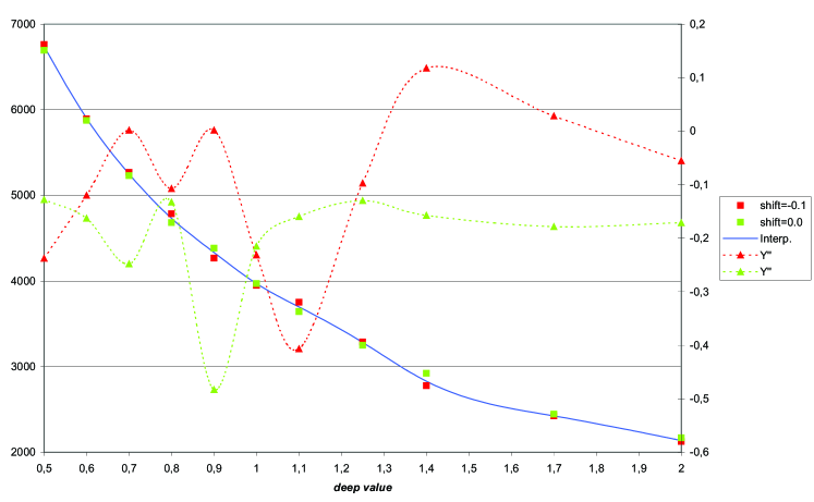
Figure 3: Graph of two functions, $Y(\mbox{shift}=-0.1\,\mbox{eV},\mbox{depth})$ given by the red squares and $Y(\mbox{shift}=-0.0\,\mbox{eV},\mbox{depth})$ with the green squares. The red triangles show $Y^{\prime\prime}(\mbox{shift}=-0.1\,\mbox{eV},\mbox{depth})$ , whereas the green ones stand for $Y^{\prime\prime}(\mbox{shift}=0.0\,\mbox{eV},\mbox{depth})$. The green solid line is obtained by an interpolation function for a shift value of $-0.05$ eV.

3 Application of the method

3.1 Description of the experiment

In this section we apply our analysis method to the data obtained in the E742 experiment performed at TRIUMF, Vancouver (Canada). The experiment was dedicated to the study of $\mu$-atomic processes occurring in solid hydrogen isotopes. It is of particular interest to obtain the characteristics of the interacting systems (collision energy of muonic atoms with a crystalline structure). We want to reconstruct the energy dependence of the elastic scattering cross-sections for muonic atoms in the process: $d\mu+p\to d\mu+p$ on crystalline hydrogen at a temperature of 3 K. Theoretical calculations [chicc92] postulated that there exists an energy region of abnormally small cross-section called the Ramsauer–Townsend (R–T) region. Figure 4 shows this dependence and the R–T region is visible. The aim of the measurement was to find experimentally the R–T region and verify the theoretical prediction. The accuracy of the theoretical calculations was low for energies inside the R–T region and the R–T minimum was also determined by theoretical calculations of poor accuracy. We assumed only that the general shape of the cross-section curve was valid. We vary only the depth and the position of the minimum of the R–T region.

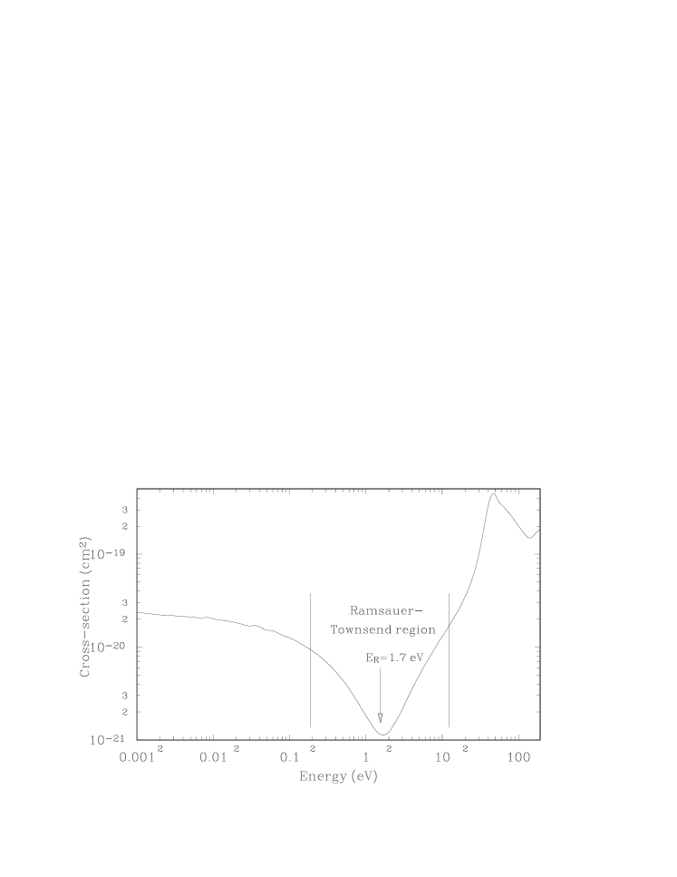
Figure 4: Elastic scattering cross-sections for $d\mu+p$ and R–T region. The essential values used in the parametrization are given.

The most accurate experimental method would be the use of a (selectable) monoenergetic beam of muonic $d\mu$ atoms, and, by aiming the beam at a thin foil of crystalline hydrogen and (like in the Rutherford experiment) detecting the intensity and energy of the scattered $d\mu$ atoms would allow us to determine the cross-section as a function of the $d\mu$-atoms energy. The method would also give us the scattering angles, and interpreting the data would be easy. However, even in this maximally simplified case it is most probable that the MC method have to be used.

Unfortunately, it is impossible to use the direct method because such a source of $d\mu$ atoms does not exist and there are no detectors measuring directly the energy of muonic $d\mu$ atoms. Therefore, in the real experiment we produced muonic atoms inside a structure of solid hydrogen, starting a time counter on the muon arrival. The energy of the scattered $d\mu$ atoms after leaving the crystal is measured indirectly via a time of flight method. The muonic atom flew between two layers placed at some distance between each other in vacuum. The first layer is a source of muonic atoms and is treated as an emitter of $d\mu$-atoms. The second layer is covered by neon and is treated as the detector of muonic atoms: a $d\mu$ atom entering the neon layer transfers the muon to the Ne almost immediately yielding an x ray which determined the stop of the time counter. Detailed information about the experiment can be found in Ref. [mulha01] and references therein.

To analyze the experiment, we have to use MC simulations because other processes are competing with the scattering, as well as the complications coming from the geometry of the experiment. Figure 5 presents the scheme of the processes taken into account [wozni96]. The initial time is given when a muon enters the apparatus. The output of the simulation is a x–ray time spectrum (see processes in external layers) which can be directly compared with the experimentally measured one.

Figure 5: Scheme of FOW program used to simulate the E742 experiment. Four process blocks are shown, namely the processes in external layers, the muon stopping, the diffusion, and the muonic processes.

3.2 The grid construction

The grid method is illustrated for one chosen set of three experiments with different experimental conditions. Since the scattering cross-section does not depend on experimental conditions, fitting three different conditions with the same parameters should reduce systematics. The theoretical dependence of the cross-section from the collision energy was parametrized on two ways. One changes the position of the minimum on the energy axis (varying $\Delta E$) and the depth of R–T minimum (varying $s$). In our example $p_{1}$ represents the shift of R–T energy ($\Delta E$) as can be seen in Figs. 4 and 6. The parameter $p_{2}$ represents a rescaling factor $s$ of the minimal cross-section value (see Figs. 4 and 8). The function $M$ is the MC time spectrum of muonic atoms reaching the neon layer for $\Delta E$ and $s$. Thus, the grid is defined as $\{M_{\Delta E_{\alpha},s_{\beta}}\}$.

3.2.1 Change of the R–T minimum energy

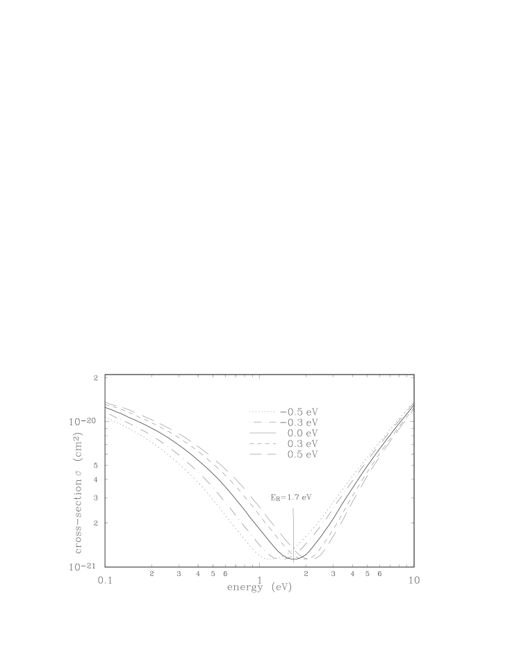
Figure 6: $\Delta E$-parametrization of the R–T position minimum. Curves for some value of $\Delta E$ are shown.

Table 1: Characteristic values used in the cross section parametrization.

Notation	Name	Value	Units
$E_{R}$	Energy of R–T minimum	1.7	eV
$E_{min}$	Minimum of energy range	0.001	eV
$E_{max}$	Maximum of energy range	190.5	eV
$\sigma(E_{R})$	Minimum cross section for the R–T energy	$1.13\times 10^{-21}$	$\mathrm{cm}^{2}$

The energy axis is transformed according to $E\to E_{tr}$ and then $\sigma(E)\to\sigma(E_{tr})$. The energy transformation are done via

$$E_{tr}=\left\{{{\begin{array}[]{*{20}c}{\begin{array}[]{l}E+\frac{E-E_{\min}}{E_{R}-E_{\min}}\cdot\Delta E,\qquad\mbox{for}\quad E\leq E_{R}\\ \\ \end{array}\hfill}\\ {E+\frac{E_{\max}-E}{E_{\max}-E_{R}}\cdot\Delta E,\qquad\mbox{for}\quad E>E_{R}\hfill}\\ \end{array}}}\right.$$ (11)

where $\Delta E$ is the energy shift, $E$ the unshifted energy, and $E_{R}$ the original value of the R–T energy minimum. Limits $E_{min}$ and $E_{max}$ define the range where the transformation is applied. For $E=E_{R}$ the transformed energy $E_{tr}$ given by Eq. (11) becomes $E_{tr}=E+\Delta E$, and thus, this parametrization can be treated as a shift. Characteristic values for theses variables are given in Table 1.

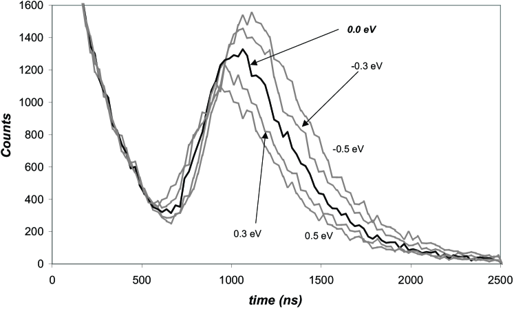
Figure 7: $M_{\alpha}(\Delta E)$, the time spectra for the shift-parametrization and $s=1$. Curves are shown for the same values as given in Fig. 6.

The shift values, $\Delta E$, were defined as 11 points between $-0.5$ eV to $0.5$ eV, in steps of $0.1$ eV. These values were chosen as a result of previous tests of the experimental data with different shift values. The shape of the cross-section curves are presented on Fig. 6. The resulting MC time spectra for such parametrized cross-section are presented in Fig. 7.

3.2.2 Change of the R–T depth minimum

The curves for the depth parametrization have a rescaled minimum cross-section $\sigma(E_{R})=s\times\sigma(E_{R})$. The rescaling took place in the energy range $0.5-6$ eV, with 11 values of the rescaling parameter $s$ chosen from 0.5 to 1.1 by steps of 0.1, with additional values of 1.25, 1.4, 1.7, and 2.0, as can be seen in Fig. 8.

Figure 8: Depth-parametrization of the R–T minimum depth. Some values of $s$, which concern the minimum cross section $\sigma(E_{R})$ are indicated.

To preserve the smooth form of the cross sections, values within the 0.5–6 eV range were not globally scaled by $s$, but were scaled by a factor which ranged from 1 at the borders, to $s$ at the energy of the R–T minimum. The $s$ values (except the minimum value) were selected numerically to reproduce the characteristic shape of the cross-section function inside the R–T region, as shown in Fig. 9. The MC time spectra for the depth parametrized cross-sections are presented in Fig. 9. The functions $M_{\alpha}(\Delta E)$ and $M_{\alpha}(s)$ given in Figs. 7 and 9, respectively, were combined and a grid $\{M_{\alpha,\beta}(\Delta E,s)\}$ was created.

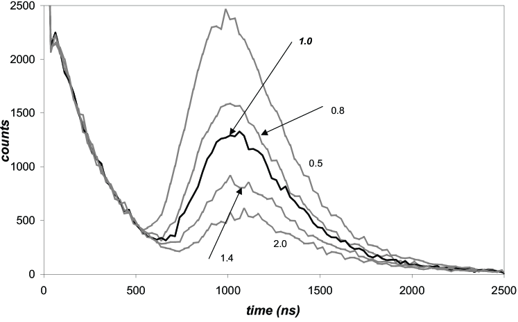
Figure 9: $M_{\beta}(s)$, the time spectra for the depth parametrization, without the energy shift $\Delta E=0$.

4 The results

An example of the experimental data fits using the MC time spectra (see Figs. 7 and 9) is presented in Fig. 10. In this case three sets of experimental data (called Expositions 1–3) were fitted. Fits were performed for a number of data combinations.

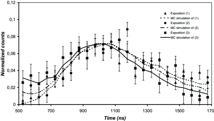
Figure 10: Example of a fit.

The average values from all possible fit combinations give the final result:

$$s=1.12\pm 0.20\,,\qquad\Delta E=0.30\pm 0.14\,\mbox{eV.}$$ (12)

The errors are connected with low experimental statistics, some background problems, and also with the grid steps (0.10 eV for $\Delta E$ and $0.1-0.15$ for $s$) and finally with the interpolation procedure. The result means that our experimental result confirms the theoretical cross-section energy dependence in the R–T region, but indicates that the minimum of the cross-section value occurs for energies higher than predicted, at about 2 eV instead of 1.7 eV in Fig. 4. The absolute value of the fitted cross-sections agree with the theoretical value.

5 Conclusion

The method allowed us to perform a correct comparison of experimental data with theoretical predictions based on MC calculations. Although the experimental data was obtained in only a few weeks of muon beam usage, the grid construction was a time-consuming step requiring more than six months of calculation. The fitting procedure was quick and allowed us to prepare many fits for any combination of the data and perform more complex analysis of the data themselves, e.g., $\chi^{2}$–contour and error calculations.

To establish a more precise set of mathematical rules which test the correctness of this method, one needs to perform further studies but such was not the aim of this work. The grid method, as demonstrated here, is fully acceptable for analyzing systems with complex multiparameter dependences. Our procedure was internally checked by comparing results of fitting single and summed data. The errors of single data fits are bigger but they lie within the range of the experimental errors of summed data.